Supervised principal component analysis for gene set enrichment of microarray data with continuous or survival outcomes

Abstract

Motivation: Gene set analysis allows formal testing of subtle but coordinated changes in a group of genes, such as those defined by Gene Ontology (GO) or KEGG Pathway databases. We propose a new method for gene set analysis that is based on principal component analysis (PCA) of genes expression values in the gene set. PCA is an effective method for reducing high dimensionality and capture variations in gene expression values. However, one limitation with PCA is that the latent variable identified by the first PC may be unrelated to outcome.

Results: In the proposed supervised PCA (SPCA) model for gene set analysis, the PCs are estimated from a selected subset of genes that are associated with outcome. As outcome information is used in the gene selection step, this method is supervised, thus called the Supervised PCA model. Because of the gene selection step, test statistic in SPCA model can no longer be approximated well using t-distribution. We propose a two-component mixture distribution based on Gumbel exteme value distributions to account for the gene selection step. We show the proposed method compares favorably to currently available gene set analysis methods using simulated and real microarray data.

Software: The R code for the analysis used in this article are available upon request, we are currently working on implementing the proposed method in an R package.

Contact: chenx3@ccf.org.

1 INTRODUCTION

Microarray technology has been used extensively in biological and medical studies to monitor thousands of genes at the expression level across the genome. Typically, statistical analysis for microarray calculates P-values for each gene based on a statistical test first, and then applies multiple comparison methods to adjust the nominal P-values. When many significant genes are selected, it is often difficult to interpret the results in biological context. On the other hand, due to the large number of genes tested, it may also be possible that too few significant genes are left after adjusting for multiple comparisons.

Gene set analysis tests for expression changes in groups of related genes in microarray data, such as those defined by gene annotation databases Gene Ontology (GO) (Ashburner et al., 2000) and KEGG Pathway (Kanehisa and Goto, 2000). In additional to facilitate interpretation of results, gene set analysis also increases power by combining weak signals from a number of individual genes in the group.

Software packages such as GENMAPP (Dahlquist et al., 2002), CHIPINFO, ONTO-TOOLS (Draghici et al., 2003), GOstat (Beibbarth and Speed, 2004), DAVID (Dennis et al., 2003), WebGestalt (Zhang et al., 2005), GOTM (Zhang et al., 2004), JMP Genomics (http://www.jmp.com/genomics) and GeneTrail (Backes et al., 2007) use various approaches to test for overrepresentation of significant genes that belong to a gene set. A full discussion of the methods and a detailed comparison of these tools can be found in Khatri and Draghici (2005). Rivals et al. (2007) discussed different sampling designs that can lead to the hypergeometric null distribution and details on the implementation of the methods. Despite its popularity, there are a number of limitations with overrepresentation analysis: the assumption that genes are independent may not hold for tightly co-regulated gene sets; the selection of significant genes is often based on an arbitrary cutoff; and information is lost by not using continuous information in P-values.

One method that uses the continuous distribution of P-values is the Gene Set Enrichment Analysis (GSEA) method (Mootha et al., 2003; Subramanian et al., 2005). GSEA makes statistical inference by permuting sample labels, thus preserving correlation structure among genes. Some extensions of the GSEA method include GSA (Efron and Tibshirani, 2007), SAM-GS (Dinu et al., 2007), GSEA via dynamic programming (Keller et al., 2007), GSEAlm (Jiang and Gentleman, 2007). Other permutation-based methods, include SAFE (Barry et al., 2005), multivariate N-statistic (Klebanov et al., 2007) and others. Some recently proposed parametric methods that do not rely on permutation test, include PAGE (Kim and Volsky, 2005), GlobalTest (Goeman et al., 2004, 2005), GlobalANCOVA (Hummel et al., 2008), Mixed models (Wang et al., 2008) and others.

Most of the aforementioned algorithms had been presented as tests for association of gene sets with binary outcomes. In practice, microarray experiments may also have continuous outcome for quantitative traits such as lesion score or body weight. In the field of cancer research, the outcome is often survival time or time to death, to avoid arbitrary cutoff such as 10 years survival, the analysis needs to account for censored observations. Censoring occurs, for example, when the patients survived over the entire study period or were lost to follow-up; in these cases, we only know partial information on the outcome. One way to analyze microarray dataset with survival outcome using Fisher's exact test is to fit Cox regression model for each gene (with its gene expression value as predictor) and then use a predetermined cutoff (e.g. P-value<0.05) based on P-values from Cox model as threshold for declaring differential gene expression. Similarly, GSEA can also be adapted for microarray experiments with continuous or survival outcome by using linear regression or Cox regression model instead of t-statistics to obtain local statistics for each gene. However, the performance and properties of these tests for continuous or survival outcomes had not been adequately studied.

In this article, we propose a new gene set analysis method for testing association between sets of genes with continuous or survival outcomes. We evaluate its performance and compare it to performance of tests in currently available tools, such as Fisher's exact test, GSEA and extensions of GSEA. In addition, we illustrate this new method using data from two microarray experiments with lesion score and survival outcomes. This new method extends methods in Tomfohr et al.,(2005), Bair and co-workers (2004, 2006). Tomfohr et al. (2005) performed principal component analysis (PCA) on gene expression values from an a priori defined gene set, estimated correlation statistic between continuous outcome and the first PC, and then tested association between gene sets and outcome using a permutation test. Although PCA is an effective method for reducing high dimensionality and capture variations in gene expression values (Alter et al., 2000), one limitation is that the latent variable identified by the first PC may be unrelated to outcome.

Instead of performing PCA on all genes, Bair and co-workers (2004, 2006) proposed supervised PCA (SPCA) method, which estimated PCs from a selected subset of genes. Because outcome values were used to select the subset of genes, this procedure is supervised, and thus called SPCA. The SPCA method was shown to be an effective algorithm for classification of survival and continuous outcomes using gene expression data. The estimation of PCs from a selected subset of genes significantly improved prediction accuracy in SPCA algorithm compared to the PCA algorithm without the gene screening step. Similarly, in the classification of biological samples setting, Dai et al. (2006) showed partial least squares and sliced inverse regression, which uses outcome information to construct predictors, performed better than unsupervised PCA in terms of prediction accuracy.

In this article, we extend the SPCA method to gene set analysis setting to test for significant association of a gene set with outcome. In Bair and Tibshirani (2004), the subset of genes used to estimate latent variable was selected from all the genes on a microarray. In contrast, here we select subset of genes from an a priori defined group of genes, for example, those with the same Gene Ontology (GO) term. A linear model with PC score constructed with the selected genes as predictor (see details in Section 2.2) is then used to test for association between gene set and outcome. Because of the step to select subset of genes, the resulting test statistics for regression coefficient in the proposed linear model can no longer be approximated well using t-distribution, to account for this, we propose a mixture model of extreme values to approximate distributions of the test statistic. The details of the proposed mixture model and SPCA for testing association between gene set and outcome are discussed in Section 2. In Section 3.1, we show that this method performs favorably compared to the unsupervised PCA model, Fisher's test, GSEA and its extension GSEAlm for gene set analysis using simulated data. The proposed SPCA model provides the ability to model and borrow strength across genes that are both up and down in a gene set. In addition, it operates in a well-established statistical framework and can handle design information, such as covariate adjustment, matching information and testing for interaction of effects. In Sections 3.2 and 3.3, we illustrate the SPCA model using real microarray datasets with continuous outcome lesion score and survival outcome time to metastasis of cancer. In Section 4, we provide some concluding comments.

2 METHODS

2.1 Principal component analysis

Consider a gene set with p genes, let x=(x₁ x₂…x_p)^t be a p × 1 vector, where x_i is random variable for gene expression values of the i-th gene, t denotes transpose of a vector. Let Σ be covariance matrix of x with dimension p × p, the eigenvectors and eigenvalues of Σ are defined as vectors α_ι and scalars λ_i such that Σα_ι=λ_iα_ι, i=1,…, p.

The first PC score (PC1) is a scalar defined as the linear function α₁^tx=α₁₁x₁+α₁₂x₂+···+α_1p x_p of elements of xhaving the maximum variance among all linear functions of x (Jolliffe, 2002). Without loss of generality, assuming λ₁≥λ₂≥···≥λ_p, then it can be shown the vector of coefficients α₁ for the first PC score is the eigenvector corresponding to largest eigenvalue of Σ and var(α₁^t x)=λ₁. The set of coefficients {α₁₁,…,α_1p} are sometimes called the loadings of the first PC.

The estimation of coefficients {α_ι; i=1,…,p} (eigenvectors) for PC scores on a set of genes can be computed using singular value decomposition (SVD) (Jolliffe, 2002). Briefly, let X be a N × p matrix with columns corresponding to standardized gene expression values (with mean 0 and variance 1) of a group of genes, so there are N samples and p genes. The k-th PC score is z_k=X α_k where α_k is unit length eigenvector of covariance matrix S=X^t X/(N−1) corresponding to k-th largest eigenvalue λ_k, and var(z_k)=λ_k.

Let r=rank(X). The SVD of X is

(1)

where is an N × r matrix, where u_k=l_k^−1/2 Xα_k is scaled k-th PC score, these are linear combinations of gene expression values corresponding to columns of matrix X. is an r × r diagonal matrix where l_k is k-th eigenvalue of X^t X, is a p × r matrix where α_k is eigenvector of covariance matrix S, which are also coefficients for defining PC scores. Note that since k-th eigenvalue of covariance matrix S is λ_k=l_k/(N−1), we have var(u_k)=1/(N−1).

Therefore, SVD provides not only the coefficients and SDs for the PCs with L and A matrices, but also the PC scores of each observation with matrix UL. For simple models, it can be shown that the PCs provide an optimal approximation to the original variables (Jolliffe, 2002).

2.2 SPCA model

The assumption behind the SPCA model is that given an a priori defined group of genes, only a subset of these genes is associated with a latent variable, which then varies with outcome. This assumption is based on the fact that because gene sets are defined a priori and are biological context free, when they are put into a specific biological context such as those in a microarray study (e.g. a specific tissue type or a specific disease), typically only a subset of genes from the gene set is responsible for the corresponding cellular process.

Because the subset of genes is selected using outcome information (see details below), SPCA is a supervised procedure. Biologically, a subset of genes from an a priori defined gene set, each contributing a different amount, work together to bring about changes in a cellular process, and this cellular process then relates to variations in phenotype. Therefore, our objective is to select the subset of relevant genes, estimate latent variable associated with underlying cellular process, and assess statistical significance of association between latent variable and outcome. To this end, we propose the following SPCA model:

(2)

Here, Y_j is outcome value for j-th sample, PC1 is the first PC score estimated from selected subset of genes in a predefined gene set G, it represents the latent variable for the underlying biological process associated with this group of genes. Magnitude of loadings for the first PC score can be viewed as an estimate of the amount of contributions from different genes. In the literature, the first PC score has also been called ‘eigengene’ (Alter et al., 2000). With Model 1, statistical significance of would indicate significant association between gene set G and outcome.

Given a set of gene expression values G={x₁, x₂,…,x_p} for an a priori defined gene set, the selection for the subset of relevant genes can be accomplished in several steps:

(1) For each gene, compute an association measure ρ_i with outcome by fitting linear or proportional hazard models for continuous or survival outcomes, with values for the gene as predictor. For example, for linear regression, let x_ij be gene value for i-th gene and j-th sample, we fit model Y_j=β_i0+β_i1 x_ij+ɛ_ij and use (s.e. denotes standard error) as the association measure.

(2) Predetermine a set of n threshold values {t₁, t₂,…,t_n}.

(2) For a given threshold value t_k, let Λ_k={x_i⊆G: |ρ_i| > t_k, i=1,..,p} be the subset of genes with magnitude of association measures above it. Compute first PC score PC1 using only genes in Λ_k and fit Model 1.

(3) Let be the t-statistic, or the standardized regression coefficient. So for the n threshold values, we have n t-statistics {T₁, T₂,…,T_n}. Let and we choose the subset of genes corresponding to threshold M.

2.3 Significance testing

Without the gene selection process, when all the genes in an a priori defined gene set are included in analysis, the test statistic in Model 1 follows t-distribution. However, for SPCA model, after gene selection step in Section 2.2, the test statistic can no longer be approximated well using t-distribution. We next show the distribution of M follows a two-component mixture distribution based on Gumbel extreme value distributions.

The Gumbel extreme value distributions model maximum or minimum of a set of random variables. More specifically, given a set of random variables {T₁, …, T_n}, under regularity conditions (Leadbetter et al., 1982), it can be shown that the maximum follows the Gumbel max distribution with distribution function F(t)=exp(−e^−z₁) and probability density function f(t)=(1/σ₁)exp(−z₁−e^−z₁) where z₁=(t-μ₁)/σ₁. Similarly, it can be shown that the minimum follows the Gumbel min distribution with distribution function F(t)=1−exp(−e^z₂) and density function f(t)=(1/σ₂)exp (z₂−e^z₂) where z₂=(t−μ₂)/σ₂.

Now, for a given gene set, let (the test statistic in Step 4 of Section 2.2), and let p=Pr(M>0), then the distribution function for M can then be approximated as

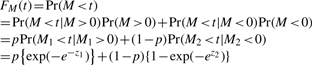(3)

The conditioning argument in the third line above follows because if M is positive, then M must be the maximum of all standardized regression coefficients {T_k; k=1, …, n}, so M=M₁ and it can be approximated with Gumbel max distribution. Similarly, if M is negative, then M must be the minimum of all {T_k; k=1,…,n}, so M=M₂ and it can be approximated with Gumbel min distribution.

The corresponding density function for M is then

(4)

Given null distribution of M (values of M corresponding to null gene sets) and formula f(t), one can easily estimate parameters p, μ₁, μ₂, σ₁, σ₂ using any non-linear optimization routine. We used R function optim for the analysis in this study. These estimated parameters can then be substituted into the formula for distribution function to calculate P-values.

For real microarray datasets, one does not know which gene set is null. One way to deal with this issue is for each gene set from microarray dataset, randomly generate phenotype values from the same assumed distribution as observed phenotype and then fit Model 1. Pooling M values corresponding to all gene sets, we then have null distribution for M. Because the phenotype values were generated randomly, without looking at the gene expression values, the resulting test statistics for M represent null distributions of M. The parameters for mixture model p,μ₁,μ₂,σ₁,σ₂ can then be estimated from this null distribution. We illustrate this procedure with two examples in Section 3.2 for microarray datasets with continuous and survival outcomes.

Once we obtain nominal P-values, we next calculate adjusted P-values using the R multtest package to control for false discovery rate (FDR)

using the method of Benjamini and Hochberg (1995). An adjusted P-value of 0.05 for a gene set indicates that among all significant gene sets selected at this threshold, 5 out 100 of them are expected to be false leads.

3 RESULTS

3.1 Simulation study

We performed a simulation study to assess the sensitivity and specificity of the SPCA model compared with PCA, Fisher's exact test, GSEA and GSEAlm methods. For each scenario in Table 1, we first generated 50 phenotype scores, corresponding to 50 samples, from normal distribution with mean 1 and SD 1. Next, for each sample, we generated 2500 gene expression values from the standard normal distribution. These gene values were then assigned to 50 gene sets, each with 50 genes.

Table 1.

Simulation study results comparing SPCA, PCA, GSEA, GSEAlm, and Fisher's Exact Test

Scene	N_Genes	r_mean	r_variance	Area Under Curve						Av.p-value for Gene Set 1
				SPCA	PCA	GSEA	GSEAlm	Fisher (0.05)	Fisher (0.1)	SPCA	PCA	GSEA	GSEAlm	Fisher (0.05)	Fisher (0.1)
1	5	0.1	0.5	0.898	0.758	0.740	0.567	0.674	0.699	0.059	0.410	0.259	0.428	0.656	0.606
2	5	0.1	1	0.956	0.716	0.780	0.566	0.825	0.849	0.028	0.271	0.219	0.427	0.358	0.308
3	5	0.1	1.5	0.973	0.850	0.799	0.557	0.900	0.899	0.018	0.146	0.203	0.436	0.205	0.206
4	5	0.2	0.5	0.895	0.572	0.727	0.614	0.749	0.774	0.060	0.417	0.275	0.380	0.508	0.459
5	5	0.2	1	0.947	0.740	0.781	0.604	0.875	0.874	0.032	0.250	0.219	0.389	0.260	0.259
6	5	0.2	1.5	0.963	0.848	0.758	0.604	0.890	0.899	0.022	0.147	0.219	0.387	0.205	0.206
7	10	0.1	0.5	0.962	0.707	0.788	0.613	0.775	0.774	0.025	0.283	0.211	0.383	0.458	0.458
8	10	0.1	1	0.993	0.902	0.840	0.612	0.925	0.924	0.006	0.092	0.158	0.384	0.157	0.154
9	10	0.1	1.5	0.999	0.980	0.908	0.600	0.975	0.975	0.001	0.019	0.087	0.394	0.054	0.053
10	10	0.2	0.5	0.965	0.714	0.857	0.710	0.850	0.874	0.023	0.277	0.140	0.282	0.311	0.262
11	10	0.2	1	0.995	0.887	0.868	0.700	0.925	0.924	0.006	0.110	0.129	0.294	0.156	0.153
12	10	0.2	1.5	0.999	0.995	0.887	0.678	0.975	0.999	0.001	0.005	0.113	0.316	0.053	0.004

Fisher(0.05) = Fisher's exact test using 0.05 FDR level as significance level cutoff; Fisher(0.1)=Fisher's exact test using 0.1 FDR level as significance level cutoff; r_mean=mean of association measure r; r_variance=variance of association measure r; see text for details of simulation experiments.

For gene set 1, treatment effects for a subset of genes (n_genes in Table 1) were added according to parameter r_i ∼ N(μ_r,σ_r²), which corresponds to association between expression values of i-th gene with phenotype score. Let x_j represent the phenotype score for sample j, the gene expression value y_ij for i-th treated gene from gene set 1 for sample j were generated as y_ij=r_i x_j+ɛ _ij where ɛ_ij ∼ N(0,τ²). Under this setup, genes in the first gene set can be either positively correlated with phenotype (up-regulated with r_i>0) or negatively correlated with phenotype (down-regulated with r_i<0). The remaining genes in gene set 1 and other gene sets are control genes, they were generated from N(0,τ²).

Therefore, for each scenario in Table 1, by design of the experiment, only the first gene set was associated with phenotype and the other gene sets were null gene sets. There were 12 (=2×2×3) scenarios: the numbers of genes in gene set 1 with treatment effects added were 5 or 10 genes; μ_r (mean for r_i)=0.1, 0.2; σ_r² (variance for r_i)=0.5, 1, 1.5; and the SD for noise ɛ _ij was set to be τ=3.

To compare the performances of SPCA, PCA, Fisher's exact test, GSEA, GSEAlm algorithms, for each scenario, we generated 20 datasets, each with 2500 gene expression values and 50 phenotype scores as described above. For each method, using gene sets from all 20 datasets (49×20=980 control gene sets, and 1×20=20 gene sets associated with outcome), we computed receiver operator characteristics (ROC) curves which show the tradeoff between sensitivity and 1 - specificity as the threshold for declaring significant gene set was varied. To compare the overall discriminative abilities of the methods over all possible cutoffs, we calculated the area under the ROC curve (AUC). In addition, to compare sensitivity of the methods, we calculated the mean of P-values for gene set 1.

The javaGSEA implementation was used for GSEA analysis, we chose ‘Pearson correlation’ (between expression values and phenotype scores) as the metric for ranking genes and 200 permutations were applied to phenotype labels. For SPCA, unsupervised PCA, GSEAlm and Fisher's exact test methods, we used R packages (http://www.r-project.org/) superpc (with modification), lm, GSEAlm, and fisher.test.

In terms of AUC, the results in Table 1 show that the SPCA model outperformed the PCA and GSEA models consistently

across all scenarios, especially when the variance of r_i is small. P-values for gene set 1 from the SPCA model were smaller than the other methods for all scenarios indicating higher sensitivity for this method. GSEAlm which tested mean shift of r_i from zero for genes from each gene set did not perform well, probably because signals from up-regulated genes with positive r_i canceled signals from down-regulated genes with negative r_i. In contrast, the good performance from SPCA method shows this method can be used to effectively model reverse regulations in gene sets where both up- and} down-regulated genes are expected. Figure 1 shows the ROC curves for the six methods for scene 4 in Table 1. Fisher's exact tests showed very good specificity: for example, when FDR 0.05 was used as threshold for selecting significant genes, for 980 null gene sets, Fisher's exact test estimated gene set P-values to be 1 for all gene sets except one gene set with P-value 0.04. Therefore, the probability of false positive, or 1 - specificity, based on null gene sets, had only three values: 0, 1/980 and 1. The points with false positive rate 1/980 and 1 were connected using a straight dotted line. Similar behavior was observed for Fisher's exact test with FDR 0.1 as threshold. On the other hand, because of this conservativeness, sensitivity for Fisher's exact test is also compromised. Figure 1 shows among all methods, SPCA method had the best sensitivities across all levels of specificity.

Fig. 1.

Comparison of performances of SPCA, PCA, GSEA and Fisher's exact test using simulated data. This figure shows the ROC for the methods SPCA, PCA, GSEA and Fisher's exact test for scene 4 in Table 1. Fisher (0.05)=Fisher's exact test, using FDR 0.05 as significance cutoff for differential expression of single genes. Fisher (0.1)=Fisher's exact, using FDR 0.1 as significance cutoff for differential expression of single genes. There were 20 simulated datasets, each dataset has 2500 genes assigned to 50 gene sets, among them only the first gene set include genes associated with outcome by design. See text for details of simulation experiment.

3.2 Breast cancer dataset

We applied the SPCA, GSEA and Fisher's exact test to data from a breast cancer microarray experiment (Wang et al., 2005). In this experiment, tumor samples from 286 patients with lymph-node-negative} breast cancer were collected. These patients were treated with surgery or radiotherapy over an 11 years period. The outcome of this study is time to metastasis, and our objective was to identify gene sets associated with this survival outcome. To avoid arbitrary cutoff, such as 5-year relapse-free, and to account for patients who were lost to follow-up, we used Cox regression models from survival analysis instead of logistic regression to obtain local statistics for SPCA, GSEA and Fisher's exact methods, see details below.

The expression data with 22 283 transcripts were obtained from Affymetrix U133a GeneChip platform (GEO Accession No. GSE2034). We first mapped these transcripts to EntrezGene ID and then associated them with GO biological process categories. In order to reduce the redundancy in GO, we further removed all child categories if corresponding parent category was within the size limitation between 5 and 300. After these steps we were left with 11 609 genes and 372 GO categories.

For GSEA method, we first applied Cox proportional hazards regression model to each gene, with time to metastasis as outcome and gene expression value as predictor. Next, all genes were ranked according to standardized regression coefficient from this Cox model, and this ranked gene list was then used for GSEA ‘Pre-ranked’ algorithm. Finally, 200 permutations were applied to sample labels to test if genes from each a priori defined GO gene sets were randomly distributed along the ranked gene list. Similarly, for Fisher's exact test, we applied Cox model to each gene, used FDR 0.1 as significance level cutoff to set up the two by two tables, and calculated P-values for each gene set based on hypergeometric distribution.

For the SPCA method, to generate null distribution for 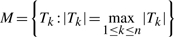, where T_k is standardized regression coefficient using the selected subset of genes (See Section 2 for details), we assumed Weibull distribution for the survival outcome time to metastasis and estimated shape and scale parameters by fitting observed outcomes from 286 patients with censoring status to intercept only Weibull survival regression model. Based on these estimated shape and scale parameters, for each gene set, we next generated a set of pseudo survival outcomes from Weibull distribution. To account for censoring, each patient was randomly chosen to have censored outcome according to the estimated censoring proportion from observed outcomes. Next, with these generated pseudo outcomes, we applied Steps 1–4 in Section 2.2 to each gene set. The resulting test statistics for M were then pooled from all gene sets to obtain null distributions of M. The parameters for mixture model p,μ₁, μ₂, σ₁, σ₂ were then estimated from this null distribution. Finally, using observed outcomes, for each gene set, we estimated P-values for test statistics in Model 1 based on this null distribution, as discussed in Section 2.3.

For all methods, once nominal P-values were calculated, the adjusted P-values were then computed using R multtest procedure to control FDR using the method of Benjamini and Hochberg (1995).

The 10 most significant GO terms found by SPCA and GSEA are listed in Table 2 and 3. At FDR 0.1 level, GSEA identified ‘translation’ as the only significant GO term. For Fisher's exact test, the lowest adjusted P-value was 0.2337 for ‘cell motility’. In contrast, SPCA identified additional 39 significant GO terms at FDR 0.1 level besides ‘translation’. In agreement with our simulation study, these results show that power for gene set analysis can be improved for GSEA and Fisher's exact test using SPCA method.

Table 2.

Ten most significant GO terms by SPCA analysis of breast cancer dataset

GO term	Size	Description	Adj P-value
0006915	281	Apoptosis	0.0198
0006412	188	Translation	0.0934
0045786	89	Regulation of cell cycle	0.0934
0000079	34	Regulation of cyclin-dependent protein kinase activity	0.0934
0019538	22	Protein metabolic process	0.0934
0006959	33	Humoral immune response	0.0934
0000075	11	Cell-cycle checkpoint	0.0934
0007126	29	Meiosis	0.0934
0030521	33	Androgen receptor signaling pathway	0.0934
0008283	272	Cell proliferation	0.0934

Table 3.

Ten most significant GO terms by GSEA analysis of breast cancer dataset

GO term	Size	Description	Adj P-value
0006412	188	Translation	0.0037
0045086	9	Positive regulation of interleukin-2 biosynthetic process	0.1300
0050772	8	Positive regulation of axonogenesis	0.1300
0045885	5	Positive regulation of survival gene product activity	0.1799
0007242	266	Intracellular signaling cascade	0.1942
0006100	5	Tricarboxylic acid cycle intermediate metabolic process	0.1942
0006044	11	N-acetylglucosamine metabolic process	0.2557
0006809	11	Nitric oxide biosynthetic process	0.3636
0019953	7	Sexual reproduction	0.3636
0042994	5	Cytoplasmic sequestering of transcription factor	0.3636

We next examined overlap of our analysis results with previous published results. Wang et al. (2005) identified a 76-gene signature for predicting tumor metastasis. These genes were selected by fitting Cox's proportional hazard models on bootstrap samples to construct multiple gene signatures that maximize area under the ROC curve (AUC) on test samples. We mapped these 76 prognostic genes to GO categories to examine their overlap with the selected gene sets from our analysis. Among the top 20 GO terms selected by SPCA, 9 of them contained genes from the 76-gene signature. However, only one of the top 20 GO terms from GSEA included genes from the 76-gene signature. The most significant GO term selected by SPCA is ‘Apoptosis’, which is known to play an important role in cancer. Two genes from this gene set, TNFSF10 and GAS2, were from the 76-gene signature of Wang et al. (2005).

To help interpret results from SPCA model, in Figure 2, for the GO term ‘apoptosis’, we plot loadings {α₁₁, α₁₂, …, α_1p} for the first PC score (Section 2.1) using a bar chart. We call these ‘Important Scores’ for the genes: the magnitude and directions of the coefficients represents contributions of each gene to the estimated PC score or the underlying cellular process approximated by the first PC score.

Fig. 2.

Gene plot for genes in GO category apoptosis from breast cancer dataset. The values on the horizontal axis are gene symbols of genes from apoptosis GO term, values on vertical axis refer to importance score for the genes, or the loadings of first PC score for a given gene. The magnitude and directions of the coefficients represent contributions of each gene to the estimated PC score or the underlying cellular process approximated by the first PC score. Genes playing more important roles in the association between apoptosis and survival outcome have larger magnitude (absolute value) for importance scores.

3.3 Mouse lesion score data

We next applied the proposed SPCA model to an eQTL study. In this section, we illustrate the proposed method for a microarray dataset with continuous outcome lesion scores, and we show this method can efficiently account for the design of experiment, by testing for interaction effects and accounting for covariate information.

To identify genetic factors associated with atherosclerosis Bhasin et al. (2008) conducted eQTL analysis using bone marrow-derived macrophages from F₂ mice obtained by a strain intercross between aopE-deficient mice on the AKR and DBA/2 backgrounds. The apoE-deficient mouse model was created by gene targeting through homologous recombination in embryonic stem cells. These mice spontaneously develop aortic lesions on a low-fat chow diet. The continuous outcome for this study was lesion score, which was used as a measure of severity for atherosclerosis. Our main objective was to identify gene sets associated with variations in lesion scores.

Affymetrix 430v2 expression data from 93 female and 114 male mice were used for this experiment (GEO Accession No. GSE8512). Each sample had 22 174 expressed transcripts. After mapping these transcripts to EntrezGene ID and associating them with GO biological process categories, there were 9744 genes, mapped to 255 GO categories.

It has been shown that mouse atherosclerotic lesion areas QTLs are sexually dimorphic (Smith et al., 2006). In this eQTL analysis only 1% trans-eQTLs were shared by both sexes, and 31% of expressed transcripts were expressed at different levels in males versus females (Bhasin et al., 2008). Therefore, for methods such as GSEA or Fisher's exact test, gene sets can only be analyzed separately using samples from each sex. In contrast, for the proposed method, we can test whether the association between first PC of the gene set with lesion score is similar for the two groups by testing interaction effect Sex × PC1(supervised first PC score of the gene set, see Section 2.2). In particular, for each gene set, we fit linear model with outcome log(lesion score), fixed effects Sex, PC1, Sex × PC1. In addition, we specify separate residual variances for each sex to allow for different variations in lesion scores for the two groups. When Sex × PC1 interaction was not significant for a gene set, samples from male and female were pooled to gain more power, otherwise we conducted test for the gene set separately for males and females using Model 1 in Section 2.2.

For gene sets with significant Sex × PC1 interaction effect (at FDR 0.1 level), we constructed separate null distributions for (Section 2.2) for male samples and female samples. For example, for male samples, we estimated mean and variance of log(lesion scores) using only male samples and then generated pseudo lesion scores from normal distribution with this estimated mean and variance. Next, with these pseudo outcomes, the steps outlined in Sections 2.2 and 2.3 were followed to calculate P-values for each gene set. Table 4 shows the three most significant gene sets for females and males. These gene sets showed a different expression pattern between females and males, and this sexually dimorphic effect could be due to exposure to the different hormonal milieu in female and male mice.

Table 4.

Three most significant gene sets identified by SPCA method for females and males, among gene sets with significant Sex × PC1 interaction

GO term	Size	Description	Adj P-value
Females
0007242	265	intracellular signaling cascade	0.0999
0006511	105	ubiquitin-dependent protein catabolic process	0.0999
0009117	24	nucleotide metabolic process	0.0999
Males
0019882	29	antigen processing and presentation	0.0802
0006811	161	ion transport	0.0802
0045449	219	regulation of transcription	0.0802

For gene sets with non-significant Sex × PC1 (at FDR 0.1 level), P-values were estimated using null distributions constructed with all samples. The 10 most significant gene sets are listed in Table 5. Previous studies have implicated these gene sets to be related to cardiovascular diseases. For example, the top one and three gene sets are ‘electron transport’ and ‘apoptosis’. The mechanisms of mito-chondrial dysfunction related to atherosclerosis had been proposed. Reactive oxygen species (ROS) are produced by the mitochondrial electron transport chain, and the increased production of ROS can result in significant damage to lipids, proteins and mtDNA, which will induce vascular smooth muscle cell apoptosis, leading to the development of atherosclerosis (Liu et al., 2002; Madamanchi and Runge, 2007). The second most significant gene set is ‘chloride transport’, in which three genes, Slc12a5, Clcn4-2 and Clnsla were among genes in the selected subset. The K–Cl cotransporter had been identified as part of the SLC12 family and is directly related to ROS generation and oxidative stress (Adragna and Lauf, 2007).

Table 5.

Ten most significant gene sets identified by SPCA method, among gene sets with non-significant Sex × PC1 interaction

GO term	Size	Description	Adj P-value
0006118	220	electron transport	0.0114
0006821	19	chloride transport	0.0114
0006915	259	apoptosis	0.0114
0046777	37	protein amino acid autophosphorylation	0.0114
0007275	291	multicellular organismal development	0.0114
0009887	61	organ morphogenesis	0.0114
0018107	6	peptidyl-threonine phosphorylation	0.0114
0030154	173	cell differentiation	0.0114
0007067	112	mitosis	0.0114
0006629	111	lipid metabolic process	0.0114

4 DISCUSSION

In this article, we have described a new strategy for testing significant association of an a priori defined sets of genes with continuous or survival outcomes. Typically, only a subset of genes in the group is associated with a biological process. Therefore, without a gene screening step, when all genes in an a priori defined gene set are used to estimate PCs, performance of gene set analysis method using Model 1 (Section 2.2) would be adversely affected by noisy signals from irrelevant genes, especially when the gene set size is large. This is because the estimated first PC is often driven by sources of variation unrelated to outcome; in contrast, SPCA removes irrelevant genes before extracting the desired PC.

We have shown the proposed method compares favorably with currently available methods, with improved sensitivity and specificity at discriminating gene set associated with outcome from null gene sets, using both simulated and real microarray data. The proposed method operates within well-defined statistical framework so that the SPCA model can be easily extended to more complicated designs, such as time course experiments and dose response experiments with the use of linear mixed effect models in place of general linear models. In addition, it can be further extended by incorporating other forms of known biological knowledge (Khatri and Draghici, 2005). For example, ScorePage (Rahnenfuhrer et al., 2004) integrated information from co-regulation of genes and topology of pathways to test for significance of metabolic pathways; they constructed pathway scores based on co-regulation between pairs of genes weighted by their distance on the pathway graph. Similarly, Draghici et al. (2007) developed impact analysis for signaling pathways that considered crucial factors, such as the magnitude of each gene's expression change, their type and position in the given pathway and their interactions. Finally, SEGS (Trajkovski et al., 2008) searched for enriched gene sets constructed by integrating GO annotations with gene–gene interaction data from ENTREZ. Although not within the scope of this article, future studies based on these aforementioned ideas are being planned to further extend the power and potential of the proposed method.

Funding: NHLBI SCCOR (grant 1 P50 HL 077107 to X.C. and J.D.S.); NICHD (grant 5P30 HD015052-25 to L.W.); National Institutes of Health (grant 1 P50 MH078028-01A1 to L.W.); National Institutes of Health (grant U01-AA016662-02 to B.Z.).

Conflict of Interest: none declared

REFERENCES

- Adragna NC, Lauf PK. K-Cl cotransport function and its potential contribution to cardiovascular disease. Pathophysiology. 2007;14:135–146. doi: 10.1016/j.pathophys.2007.09.007. [DOI] [PubMed] [Google Scholar]
- Alter O, et al. Singular value decomposition for genome-wide expression data processing and modeling. Proc. Natl Acad. Sci. USA. 2000;97:10101–10106. doi: 10.1073/pnas.97.18.10101. [DOI] [PMC free article] [PubMed] [Google Scholar]
- Ashburner M, et al. The Gene Ontology consortium. Gene Ontology: tool for the unification of biology. Nat. Genet. 2000;25:25–29. doi: 10.1038/75556. [DOI] [PMC free article] [PubMed] [Google Scholar]
- Backes C, et al. GeneTrail – advanced gene set enrichment analysis. Nucleic Acids Res. 2007;35(Web Server Issue):W186–W192. doi: 10.1093/nar/gkm323. [DOI] [PMC free article] [PubMed] [Google Scholar]
- Bair E, Tibshirani R. Semi-supervised methods to predict patient survival from gene expression data. PLOS Biol. 2004;2:511–522. doi: 10.1371/journal.pbio.0020108. [DOI] [PMC free article] [PubMed] [Google Scholar]
- Bair E, et al. Prediction by supervised principal components. J. Am. Stat. Assoc. 2006;101:119–137. [Google Scholar]
- Barry WT, et al. Significance analysis of functional categories in gene expression studies: a structured permutation approach. Bioinformatics. 2005;21:1943–1949. doi: 10.1093/bioinformatics/bti260. [DOI] [PubMed] [Google Scholar]
- Beibbarth T, Speed T. GOstat: find statistically overrepresented gene ontologies within a group of genes. Bioinformatics. 2004;1:1–2. doi: 10.1093/bioinformatics/bth088. [DOI] [PubMed] [Google Scholar]
- Benjamini Y, Hochberg Y. Controlling the false discovery rate: a new and powerful approach to multiple testing. J. R. Stat. Soc. B. 1995;57:1289–1300. [Google Scholar]
- Bhasin JM, et al. Sex specific gene regulation and expression QTLs in mouse marophages from a strain intercross. PLoS One. 2008;3:e1435. doi: 10.1371/journal.pone.0001435. [DOI] [PMC free article] [PubMed] [Google Scholar]
- Dahlquist K, et al. GenMAPP, a new tool for viewing and analyzing microarray data on biological pathways. Nat. Genet. 2002;31:19–20. doi: 10.1038/ng0502-19. [DOI] [PubMed] [Google Scholar]
- Dai JJ, et al. Dimension reduction for classification with gene expression microarray data. Stat. Appl. Genet. Mol. 2006;5:6. doi: 10.2202/1544-6115.1147. [DOI] [PubMed] [Google Scholar]
- Dennis G, et al. David: databases for annotation, visualization and integrated discovery. Genome Biol. 2003;4:R60. [PubMed] [Google Scholar]
- Dinu I, et al. Improving gene set analysis of microarray data by SAM-GS. BMC Bioinformatics. 2007;8:242. doi: 10.1186/1471-2105-8-242. [DOI] [PMC free article] [PubMed] [Google Scholar]
- Draghici S, et al. Onto-tools, the toolkit of the modern biologist: onto-express, onto-compare, onto-design and onto-translate. Nucleic Acids Res. 2003;31:3775–3781. doi: 10.1093/nar/gkg624. [DOI] [PMC free article] [PubMed] [Google Scholar]
- Draghici S, et al. A systems biology approach for pathway level analysis. Genome Res. 2007;17:1537–1545. doi: 10.1101/gr.6202607. [DOI] [PMC free article] [PubMed] [Google Scholar]
- Efron B, Tibshirani R. On testing the significance of sets of genes. Ann. Appl. Stat. 2007;1:107–129. [Google Scholar]
- Goeman JJ, et al. A global test for groups of genes: testing association with a clinical outcome. Bioinformatics. 2004;20:93–99. doi: 10.1093/bioinformatics/btg382. [DOI] [PubMed] [Google Scholar]
- Goeman JJ, et al. Testing association of a pathway with survival using gene expression data. Bioinformatics. 2005;21:1950–1957. doi: 10.1093/bioinformatics/bti267. [DOI] [PubMed] [Google Scholar]
- Hummel M, et al. GlobalANCOVA: exploration and assessment of gene group effects. Bioinformatics. 2008;24:78–85. doi: 10.1093/bioinformatics/btm531. [DOI] [PubMed] [Google Scholar]
- Jiang Z, Gentleman R. Extensions to gene set enrichment. Bioinformatics. 2007;23:306–313. doi: 10.1093/bioinformatics/btl599. [DOI] [PubMed] [Google Scholar]
- Jolliffe IT. Principal Component Analysis. New York: Springer; 2002. [Google Scholar]
- Kanehisa M, Goto S. KEGG: kyoto encyclopedia of genes and genomes. Nucleic Acids Res. 2000;28:27–30. doi: 10.1093/nar/28.1.27. [DOI] [PMC free article] [PubMed] [Google Scholar]
- Keller A, et al. Computation of significance scores of unweighted gene set enrichment analyses. BMC Bioinformatics. 2007;8:290. doi: 10.1186/1471-2105-8-290. [DOI] [PMC free article] [PubMed] [Google Scholar]
- Khatri P, Draghici S. Ontological analysis of gene expression data: current tools, limitations, and open problems. Bioinformatics. 2005;21:3587–3595. doi: 10.1093/bioinformatics/bti565. [DOI] [PMC free article] [PubMed] [Google Scholar]
- Kim SY, Volsky DJ. PAGE: parametric analysis of gene-set enrichment. BMC Bioinformatics. 2005;6:144. doi: 10.1186/1471-2105-6-144. [DOI] [PMC free article] [PubMed] [Google Scholar]
- Klebanov L, et al. A multivariate extension of the gene set enrichment analysis. J. Bioinform. Comput. Biol. 2007;5:1139–1153. doi: 10.1142/s0219720007003041. [DOI] [PubMed] [Google Scholar]
- Leadbetter MR, et al. Extremes and Related Properties of Random Sequences and Processes. New York: Springer; 1982. [Google Scholar]
- Lee HK, et al. ErmineJ: tool for functional analysis of gene expression data sets. BMC Bioinformatics. 2005;6:269. doi: 10.1186/1471-2105-6-269. [DOI] [PMC free article] [PubMed] [Google Scholar]
- Liu YB, et al. Generation of reactive oxygen species by the mitochondrial electron transport chain. J. Neurochem. 2002;80:780–787. doi: 10.1046/j.0022-3042.2002.00744.x. [DOI] [PubMed] [Google Scholar]
- Madamanchi NR, Runge MS. Mitochondrial dysfunction in atherosclerosis. CIRC Res. 2007;100:460–473. doi: 10.1161/01.RES.0000258450.44413.96. [DOI] [PubMed] [Google Scholar]
- Manoli T, et al. Group testing for pathway analysis improves comparability of different microarray datasets. Bioinformatics. 2006;22:2500–2506. doi: 10.1093/bioinformatics/btl424. [DOI] [PubMed] [Google Scholar]
- Mardia K, et al. Multivariate Analysis. London: Academic Press; 1979. [Google Scholar]
- Mootha VK, et al. PGC-1alpha-responsive genes involved in oxidative phosphorylation are coordinately downregulated in human diabetes. Nat. Genet. 2003;34:267–273. doi: 10.1038/ng1180. [DOI] [PubMed] [Google Scholar]
- Rahnenfuhrer J, et al. Calculating the statistical significance of changes in pathway activity from gene expression data. Stat. Appl. Genet. Mol. 2004;3:16. doi: 10.2202/1544-6115.1055. [DOI] [PubMed] [Google Scholar]
- Rivals I, et al. Enrichment or depletion of a GO category within a class of genes: which test? Bioinformatics. 2007;23:401–407. doi: 10.1093/bioinformatics/btl633. [DOI] [PubMed] [Google Scholar]
- Smith JD, et al. Atherosclerosis susceptibility loci identified from a strain intercross of apolipoprotein E-deficient mice via a high-density genome scan. Arterioscl. Throm. VAS. 2006;26:597–603. doi: 10.1161/01.ATV.0000201044.33220.5c. [DOI] [PubMed] [Google Scholar]
- Subramanian A, et al. Gene-set enrichment analysis: a knowledge-based approach for interpreting genome-wide expression profiles. Proc. Natl Acad. Sci. USA. 2005;102:15545–15550. doi: 10.1073/pnas.0506580102. [DOI] [PMC free article] [PubMed] [Google Scholar]
- Tomfohr J, et al. Pathway level analysis of gene expression using singular value decomposition. BMC Bioinformatics. 2005;6:225. doi: 10.1186/1471-2105-6-225. [DOI] [PMC free article] [PubMed] [Google Scholar]
- Trajkovski I, et al. SEGS: searching for enriched gene sets in microarray data. J. Biomed. Inform. 2008;41:588–601. doi: 10.1016/j.jbi.2007.12.001. [DOI] [PubMed] [Google Scholar]
- Wang YX, et al. Gene-expression profiles to predict distant metastasis of lymph-node-negative primary breast cancer. Lancet. 2005;365:671–679. doi: 10.1016/S0140-6736(05)17947-1. [DOI] [PubMed] [Google Scholar]
- Wang L, et al. An integrated approach for the analysis of biological pathways using mixed models. PLoS Genet. 2008;4:e1000115. doi: 10.1371/journal.pgen.1000115. [DOI] [PMC free article] [PubMed] [Google Scholar]
- Zhang B, et al. GOTree Machine (GOTM): a web-based platform for interpreting sets of interesting genes using Gene Ontology hierarchies. BMC Bioinformatics. 2004;5:16. doi: 10.1186/1471-2105-5-16. [DOI] [PMC free article] [PubMed] [Google Scholar]
- Zhang B, et al. WebGestalt: an integrated system for exploring gene sets in various biological contexts. Nucleic Acids Res. 2005;33:W741–W748. doi: 10.1093/nar/gki475. [DOI] [PMC free article] [PubMed] [Google Scholar]