Augmented training of hidden Markov models to recognize remote homologs via simulated evolution

Abstract

Motivation: While profile hidden Markov models (HMMs) are successful and powerful methods to recognize homologous proteins, they can break down when homology becomes too distant due to lack of sufficient training data. We show that we can improve the performance of HMMs in this domain by using a simple simulated model of evolution to create an augmented training set.

Results: We show, in two different remote protein homolog tasks, that HMMs whose training is augmented with simulated evolution outperform HMMs trained only on real data. We find that a mutation rate between 15 and 20% performs best for recognizing G-protein coupled receptor proteins in different classes, and for recognizing SCOP super-family proteins from different families.

Contacts: anoop.kumar@tufts.edu;lenore.cowen@tufts.edu

1 INTRODUCTION

Predicting the structure and function of a newly discovered protein sequence is one of the core problems in computational biology. An established practice is to compare the new sequence with sequences in a well-characterized database and predict the structure or function based on what is known about the sequences that closely match. FASTA (Pearson et al., 1990) and BLAST (Altschul et al., 1990) are well known methods that use dynamic programming and string matching methods to detect such protein homologs. However, these methods best detect proteins that are close homologs and thus have high-sequence similarity, while they can often fail to detect proteins that have low-sequence similarity to the known proteins in the database. Thus, more sophisticated methods to detect remote homologs which may have diverged evolutionarily and have low-sequence similarity can be required. The detection of distant homology is thus an important process both in protein structure and in protein function prediction.

One of the most successful methods to date for recognizing both close and distant homologs has been profile hidden Markov models (HMMs). Popular HMM methods such as HMMER (Eddy et al., 1998a, b) and SAM (Hughey and Krogh, 1996) have been behind the design of databases such as Pfam (Finn et al., 2006), PROSITE (Hulo et al., 2006) and SUPERFAMIILY (Wilson et al., 2007). In particular, an HMM model is trained for each protein family in the database. For a new protein sequence, the probability that it could be generated by each HMM model is calculated and the protein is assigned to the family if the P-value is below a specified cutoff.

While HMMs are a very powerful methodology, as in any machine learning method, they can only be ‘as good as the training set’—that is, an HMM will not recognize a true member of the target class that is too far from any of the training examples it has. This is completely obvious statement and in most problem domains that is the end of the story. However, the fundamental insight of this article is that in protein homology detection this need not be the end of the story, that is, we can actually harness the power of a simple evolutionary model to generate new, additional artificial training data in the case of training HMMs to recognize remote protein homologs. Surprisingly, we find that these HMMs augmented by simulated evolution can outperform the regular HMMs on this problem domain.

In particular, given a target percentage of point mutations, for each of the original training sequences, a certain number of additional training sequences are generated. They are generated using a very simple model of point mutations (Section 2.2). Then the training sequences are all aligned and HMM training proceeds as usual (Fig. 1).

Fig. 1.

Building HMM by (A) traditional approach (B) augmenting the training set with simulated evolution.

We test our method using HMMER, one of the most popular HMM methods for detecting protein sequence homology, on two datasets. The first contains the G-protein coupled receptors (GPCR) protein families previously studied by Karchin et al. (2002). GPCRs are large proteins that sense molecules outside the cell and activate transduction pathways inside the cell and ultimately cellular responses (Oliveira et al., 1993). There is enormous interest in the pharmaceutical industry to understand the structure and function of GPCR proteins in order to develop drugs that target them (Horn et al., 2000). Several groups have developed computational approaches to recognize classes and sub-classes of GPCR proteins (Cheng et al., 2005; Jaakkola et al., 2000; Karchin et al., 2002; Srivastava et al., 2007).

Second, we consider a larger benchmark dataset based on SCOP. Structural classification of proteins (SCOP), is a database that classifies all proteins based on known structure, function and sequence (Murzin et al., 2005). It is a hierarchical classification: proteins belonging to the same family have similar sequence and likely common evolutionary origin and similar function. Families that demonstrate structural or functional similarity are grouped into a superfamily. Superfamilies that have same overall secondary structure are grouped in the same fold. In this study, we are interested to know whether the HMMs that are trained on sequences from a family can detect the proteins that belong to a different family within the same superfamily.

On the SCOP dataset, we compare not only with the default HMMER weighting schemes, but also to HMMs trained with two different sets of weights based on entropy: the maximum entropy (Krogh and Mitchison, 1995) and SAM sequence entropy (Karplus et al., 1998) methods. It has been demonstrated that SAM sequence entropy can outperform default HMMs in remote homology detection tasks (Johnson, 2006).

For both datasets, we find that augmenting our training set with simulated evolution yields better sensitivity and specificity than training only on real known protein sequence examples even with either type of entropy weighting. On the SCOP dataset, we find that a hybrid method that combines SAM sequence entropy with our simulated evolution method performs best of all. All our results can be found at http://bcb.cs.tufts.edu/athmm/.

2 METHODS

2.1 Datasets

We test our methods both against traditional HMMs and, on the SCOP dataset, on HMMs modified with entropy weighting schemes, methods that aim to extract the maximum from the training data in an information-theoretic sense. The fact that our simple model of augmented evolution outperforms HMMs on our test set examples shows the power of incorporating even a little phylogenetic knowledge into HMM training. We consider the implications of this further in the Section 4.

2.1.1 GPCR dataset

We consider the GPCR dataset that was created from the set of protein sequences used by Karchin et al. (2002). These proteins are grouped into five top-level families. In addition, Karchin et al. provide a decoy set of non-GPCR proteins. The sizes of the GPCR classes along with decoy sequences in the dataset are shown in Table 1.

Table 1.

GPCR class distribution

Family	Number of Proteins	Percentage of dataset
Class A	692	78.91
Class B	56	6.39
Class C	16	1.82
Class D	11	1.25
Class E	3	0.34
Decoy	99	11.29

We considered the following problem in remote homology detection—could an HMM trained on four of the five GPCR classes recognize the sequences from the remaining class?

From the dataset, we construct the five training sets. Each set omits one class and includes the remaining four classes. For example, HMMĀ contains sequences from classes from B, C, D and E but not A. In fact, we pick up to 20 sequences (if available) of each of the four classes at random in the training set. The test set contains positive sequences from the omitted class (in this case, class A) and an equal number of negative sequences from the decoy class. The training set is available at http://bcb.cs.tufts.edu/athmm/gpcr/

2.1.2 SCOP dataset

We considered the following problem in remote homology detection: training from sequences from one family in a SCOP superfamily, can we recognize sequences in other families of the superfamily? We employed the approach of Wistrand and Sonnhammer (2004) to pick the SCOP families and train HMMs for evaluation. First, we chose sequences from SCOP that are <95% identical based on the ASTRAL database version 1.73 (Chandonia et al., 2004). (We also tested our methods with a 90% identical set and the results were stable.) The dataset was filtered to contain only the SCOP families that had at least 10 sequences for which there existed other SCOP families in the same superfamily that had at least five but not >50 sequences. The procedure produced 112 families each of which had 10–108 sequences. In this case, our test set consisted of all the sequences in the other families of superfamilies and an equal number of decoy sequences chosen at random from different SCOP folds. The dataset is available at http://bcb.cs.tufts.edu/athmm/scop/data/

2.2 A mutation model

We used the BLOSUM62 matrix as our simple model of evolutionary mutations (Eddy, 2004). Mutations in a sequence are added by randomly picking a position in the sequence and replacing the amino acid in that position with a new amino acid based on the BLOSUM62 probability until a desired threshold of t% mutations is reached. For every training sequence, 10 mutated sequences with t% mutations are created and added to the training set. Therefore, for a family with 100 sequences will have 1100 (100 original + 1000 mutated) sequences in the training set. In this study, we create training sets with 5, 10, 15, 20 and 25% mutations per the length of sequence.

2.3 Building the HMM

From the set of protein sequences that belong to a family, an HMM is built in two steps: (i) aligning the sequences and (ii) building an HMM from the alignment. In our approach, the primary steps in building the HMM remain the same except the training set is augmented with mutated sequences based on the evolutionary model. The process is shown in Figure 1.

2.3.1 Multiple sequence alignment (MSA)

This is the process of aligning the homologous residues in protein sequences into columns and thus generating a multiple sequence alignment (MSA). We used the popular program MUSCLE 3.7 (Edgar, 2004) to generate the MSA that was provided to the HMM training methods.

2.3.2 Building the HMMs

Two packages are widely adopted to work with profile HMMs: SAM (Hughey and Krogh, 1996) and HMMER (Eddy, 1998a, b). SAM has been demonstrated to be more sensitive overall, while HMMER's model scoring is more accurate (Wistrand et al., 2005). In this study, we use HMMER versions 2.3.2 and 2.4i to build and evaluate the models of protein families as it is freely available and can be easily downloaded from the web site. HMMER 2.4i was used to build HMMs that incorporate entropy based sequence weighting. We construct HMMs from the MSAs using the hmmbuild program which is part of HMMER package.

In this approach, the model of the HMM is made up of a linear set of match states, one per consensus column in the MSA. Each match state emits a single residue, with a probability score that is determined by the frequency that residues have been observed in the corresponding column of the MSA. Each match state, therefore, carries a vector of 20 probabilities, for scoring the 20 amino acids. The HMMs also model the gapped alignments by including insertion and deletion states in between the match states. The match, insertion and deletion states are connected by the transition probabilities. In our experiment, HMMER is used as black box except the constraints on choosing match states are made tighter. Using default settings, HMMER creates a match state whenever a column in the MSA has <50% gaps. We found empirically that the default cutoff was not optimal for our datasets because homology was too remote. Thus, after trying several values for the gap thresholds, we found that creating a column whenever there are <20% gaps yielded the best HMMs on our datasets. In HMMER, 3.2 this is achieved by setting the appropriate parameter; HMMER 2.4i was modified to allow this change.

By default, HMMER uses a maximum a posteriori (MAP) architecture algorithm to find the model architecture with the highest posterior probability for the alignment data. The algorithm is guaranteed to find a model and constructs the model by assuming that the MSA is correct and then marks columns that correspond to match states. An HMM is created for every MSA, thus there is a one-to-one correspondence between an MSA and an HMM, generating a library of HMMs. Therefore, for any sequence from the MSA, the HMM can be used to determine if it belongs to the MSA. In addition, the HMM can be used to check if a new sequence is similar to the sequences in the MSA and if it is then one can place the new protein in the same family. We used the default ‘glocal’ setting to construct the models, which are global with respect to the model and find multiple hits that are local with respect to the sequence. We adjusted the entropy parameters as described in the section below and left the other settings unchanged.

2.3.3 Training HMMs with maximum entropy option

In order to reduce the skewness in the distribution of sequences used to construct an HMM, HMMER supports several options to weight the sequences in training data. The default option GSC assigns lower weights to sequences that are over represented (Gerstein et al., 1994). In addition, HMMER supports the maximum entropy method that is based on information-theoretic principles. The method defines entropy of the MSA and assigns weights to the individual sequences in the MSA so as to maximize the entropy.

Assume the MSA consists of N sequences and s_ij is the character in the i-th column of the j-th sequence. The character may be an amino acid or a gap. If m^c_ij is defined to be 1 if sequence j has character c in the i-th column, or 0 otherwise, and w_j is the weight of the j-th sequence, then the weighted frequency of character c in column i is given by:

The probability of the character c in column i is given as

Krogh et al. (1995) define the distance of a sequence from the profile in terms of a probability given by

From information theory, the entropy E(w) of the distribution P(s) is given by

Thus the maximum entropy weights w^ME are defined as argmax (E(w)). Krogh et al. (1995) show that computing the weights is an easy optimization problem and weighing the sequences can correct uneven representation.

First, we built the HMMs with the default option (GSC) and then built the HMMs using the maximum entropy option for all the families in the SCOP dataset using HMMER version 2.4i.

2.3.4 Training HMMs with SAM sequence entropy

In HMMER, the match state emission probabilities are computed by combining the frequency of the observed residues with prior data about the residue types based on a nine component Dirichlet mixture prior. As the frequency of observing a residue at a certain match state increases, the effect of the prior decreases. As the residue frequency decreases the effect of the prior increases. An information-theoretic approach is employed to compute the information content of the match states and adjust the weights to obtain the desired value of information content, where the information content of match states is defined as the difference between the entropy of the profile and a random distribution. When the entropy is low, the prior is overweighted (Karplus et al., 1998).

Using the ‘entropy weighting’ option in HMMER version 2.4i, we built models with ‘-eloss’, or the loss in target information content values of 1.5, 1.3, 1.1, 0.9, 0.7 and 0.3. The models built with entropy loss (eloss)=0.7 reported the best AUC values (Table 6). Additionally, we also augmented the training set at the same time we used the entropy weighting; we call this hybrid the ‘Combined Approach’. We evaluated the models generated by default settings in HMMER, entropy settings and the models with augmented training sets. We tested the HMMs generated by all the approaches by scoring them on known sequences using the scoring method described next.

Table 6.

From this table, we can see that best parameter for SAM sequence entropy is 0.7 and for number of mutations is 20% mutations

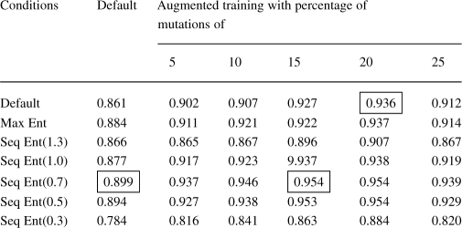Highlighted in the boxes are the best AUC values with and without the SAM sequence entropy option.

2.4 HMM scoring

Once an HMM is build from an MSA, a new sequence can be scored by the HMM. The score (S) is the log of the probability of observing

the sequence from a HMM divided by the probability of observing the same sequence from the ‘null hypothesis’ model or HMM.

P(seq|HMM) is the probability of the target sequence according to a HMM and P(seq|null) is the probability of the target sequence given a ‘null hypothesis’ model of the statistics of random sequence. In HMMER, this null model is a simple one-state HMM that says that random sequences are independently and identically distributed sequences with a specific residue composition. In addition, HMMER also generates an E-value which is the expected number of false positives with a score as high as the hit sequence. While the log odd scores provide information on the quality of a hit, the E- value gives a measure relative to other sequences. Therefore a lower E-value implies that the sequence matches more closely to the HMM.

After constructing an HMM, a cutoff for the score or E-value is set. A new sequence that lies within the cutoff is said to belong to the family that is associated with the HMM. Thus by varying the cutoff, the true positive and false positive rates of the classifier can be tuned. We run experiments over a range of cutoffs to generate receiver operating characteristic (ROC) plots that graph the tradeoffs of the true and false positives, as the cutoffs are tuned. We also compute the area under the ROC curve (AUC) to summarize the classifier statistic in a single number.

3 RESULTS

3.1 GPCR super-family recognition

We compared the performance of the HMMs on the GPCR super-family prediction problem using standard and augmented training data. As described earlier, Karchin et al.'s dataset contains proteins grouped into five families, or classes, and a set of decoy sequences. We created five datasets that represent the superfamily, where in each set, one GPCR family was omitted from the training set. The performance of the HMM was tested based on its ability to identify the sequences from the omitted family. Therefore, the test set contained sequences from the omitted family and decoy sequences that are not GPCRs. We performed ROC analysis for each case by plotting the false positive rate versus the true positive rate (Sonego et al., 2007). The ROC plots are displayed in Figures 2–6, respectively.

Fig. 2.

ROC plot for GPCR super family without class A proteins.

Fig. 6.

ROC plot for GPCR super family without class E proteins.

In addition, the AUC is computed for all the experiments and reported in Table 2. From the ROC plots and AUC statistics, it is clear that for each of the families except class A, the HMMs trained with datasets with mutated protein sequences show better performance. The HMMs trained on classes A, B C and D attempting to learn class E shows the best improvement in AUC, where the AUC goes from 0.778 for a 0% mutation rate to 1.0 for a 15–25% mutation rate. AUC decreases only in one case, and that is when class A sequences are omitted from training set. The AUC for class A goes down from 0.965 to 0.935.

Table 2.

AUC for GPCR datasets with 0, 5, 10, 15, 20 and 25% mutations

Class	0	5	10	15	20	25
A	0.965	0.911	0.922	0.952	0.947	0.935
B	0.976	0.978	0.991	0.994	0.998	0.997
C	0.969	0.906	1	0.998	0.992	1
D	0.847	0.95	0.901	0.818	1	0.904
E	0.778	0.833	0.944	1	1	1

We also calculate additional statistics and compare the classification accuracy by reviewing the coverage and average errors at minimum error point (MEP) statistics. Coverage is the percentage of true positives recognized before the first false positive occurs; it measures the sensitivity of the classifier. An average error at MEP is the score threshold at which the classifier makes fewest errors of both kinds, i.e. false positives and false negatives (Karchin et al., 2002). MEP provides a comparison of both sensitivity and specificity. Table 3 presents the coverage and Table 4 presents average errors at MEP.

Fig. 3.

ROC plot for GPCR super family without class B proteins.

Fig. 4.

ROC plot for GPCR super family without class C proteins.

Fig. 5.

ROC plot for GPCR super family without class D proteins.

Table 3.

Coverage for GPCR datasets with 0, 5, 10, 15, 20 and 25% mutations

Class	0	5	10	15	20	25
A	0.57	0.21	0.31	0.40	0.46	0.30
B	0.85	0.87	0.87	0.91	0.93	0.93
C	1.00	0.94	0.97	0.97	0.97	1.00
D	0.73	0.73	0.64	0.73	1.00	0.82
E	0.67	1.00	1.00	1.00	1.00	1.00

Table 4.

Average errors at MEP for GPCR datasets with 0, 5, 10, 15, 20 and 25% mutations

Class	0	5	10	15	20	25
A	11.11	21.46	18.18	25	13.64	21.97
B	8.75	8.75	5	3.75	3.75	2.50
C	0	6.25	3.13	0	3.13	3.13
D	9.09	6.82	4.55	4.55	0	4.55
E	16.67	16.67	0	0	0	0

From Tables 2–4, it is clear that coverage and MEP statistics concur with the ROC analysis. We observe that MEP decreases for all classes except class A. At the same time, the coverage rises; this implies that the method is good at not only reducing the false positives, but also at detecting more true positives before detecting a false positive. Again, the maximum improvement of 16.27% is observed for the class E protein set, which is the smallest set.

3.2 SCOP family recognition

We examined the classification performance of the new HMMs for the SCOP families. The SCOP dataset as described in Section 2.1 contained 112 families. Six Profile HMMs were built for each family with training sequences that contained 0, 5, 10, 15, 20 and 25% mutations. The test set was constructed with positive sequences, which belonged to the SCOP superfamily, but not the family in training set. The negative test sequences were drawn from other SCOP folds to which the family does not belong. Each family HMM was searched against the corresponding test set by the hmmsearch tool available in HMMER. The raw scores and E-values reported with the predictions were used to determine the sensitivity of the new HMM and compare them with traditional HMMs that were not trained with mutated sequences.

A ROC curve was made to analyze the results. The range of false positive rates was obtained by varying the cutoff E-values from 0 to the maximum E-value in the result set. ROC plots for all the 112 SCOP families are available at: http://bcb.cs.tufts.edu/athmm/scop/plots/. The overall plot that includes the entire set of sequences is shown in Figure 7. The plot represents the median of true positives for each false positive. From the figure, we observe that the novel HMMs built from dataset that contain mutations in the training set perform better than traditional profile HMMs.

Fig. 7.

ROC plot for SCOP families generated from dataset with 0 (mut0), 5 (mut5), 10 (mut10), 15 (mut15), 20 (mut20) and 25% (mut25) mutations.

Next, we computed the AUC for all the families. Figure 8 displays the percentage change in AUC with percentage of mutations in the datasets. It is clear that most families have an increase in AUC as the percentage of mutations rises until about a threshold of 20% mutations, and then the performance begins to degrade again. The median AUC was 0.86, 0.90, 0.91, 0.93, 0.94 and 0.90 for 0, 5, 10, 15, 20 and 25% mutation training sets, respectively. Both ROC plots and the AUC statistics confirm that profile HMMs built with percentage of mutated sequences between 20 and 25 are best at predicting the SCOP family of protein sequences.

Fig. 8.

Plot showing percentage of improvement in AUC with mutations. We observe most of the families lie above 0, implying more families show improvements when mutations are introduced into the training set.

We further analyzed the results to find out the number of SCOP families that perform better with the HMMs trained with additional data. Out of 112 SCOP families, training sets that contained mutated sequences perform better in case of 65 (58%) and the AUC is increased by 5% in 28 (25%) of families. Only in 6 (5.4%) families did the augmented HMMs have >5% decrease in AUC. We analyzed AUC further to determine the improvement in performance due to mutations. Detailed results for each individual mutation set are displayed in Table 5.

Table 5.

Number of families (FC) that show improvement with the mutated dataset. FC > 5% denotes FC whose AUC increases by at least 5%

Percentage of mutations	FC	FC > 5%
5	51 (45.5%)	14 (12.5%)
10	62 (55.4%)	26 (23.4%)
15	65 (58.0%)	28 (25.0%)
20	59 (52.7%)	19 (17.2%)
25	57 (50.1%)	21 (18.8%)

The ROC plots and AUC show an improvement in >45% of families with the 5% mutated dataset and the improvement goes up to 58.0% with the 15% mutated dataset. This proves that the HMMs can be generalized to classify sequences that were not part of the real training set by augmenting with mutated sequences. We can infer that when a profile HMM captures insufficient signal from a set of sequences, the sensitivity of the HMM can be improved by including mutated sequences in the training set.

3.3 Comparison with maximum entropy and SAM sequence entropy on the SCOP dataset

We compared the AUC reported by the HMMs generated with default settings to those generated by using the maximum entropy option and those generated by using the SAM sequence entropy at various eloss values. We also trained the HMMs with our augmented training approach and the SAM sequence entropy option at the same time, producing a combined approach. The comparison of our approach with ordinary HMMs, maximum entropy, SAM sequence entropy and the combined approach appear in Tables 6 and 7 and Figure 9. With default HMM settings, 20% mutations augmented training achieves an AUC > 93% whereas the best entropy method achieves an AUC < 90%. The best AUC is achieved by the method that combines SAM Sequence Entropy and 20% mutations augmented training for an AUC > 95%. It can be seen that our approach dominates not only the unweighted HMMs, but also the HMMs trained with SAM sequence entropy on the SCOP dataset. The combined approach of adding SAM sequence entropy to our approach has the best performance.

Table 7.

Comparison of methods with best mutation rate and eloss parameters

Method	AUC
Default (HMM with default settings)	0.8612
Maximum entropy (HMM with maximum entropy option)	0.8843
Our approach (HMM with augmented training set of 20% mutation rate)	0.9357
SAM sequence entropy weighting (eloss=0.7)	0.8994
Combined approach (HMM with augmented training with 20% mutation rate and SAM sequence entropy with eloss = 0.7)	0.9544

Fig. 9.

Performance of HMMs trained from augmented datasets with and without entropy options. Here, the mutation rates for augmented training are set to 20% and eloss for SAM sequence entropy is set to 0.7 according to the best value in Table 6.

4 DISCUSSION

We have shown that HMMs trained with datasets that are augmented with sequences based on a simple evolutionary model can better detect remote homologs than ordinary HMMs, or even HMMs reweighted by entropy approaches. The power of our new method probably comes from two things: first, by using the information in the BLOSUM62 matrix, we are incorporating phylogenetic knowledge into our training data. Second, we suspect that augmenting the training data is also dealing with entropy effects at the same time as we are adding phylogenic information. It would make sense that our approach automatically made an entropy adjustment, because the random mutations would tend to ‘smooth out’ the information across the (augmented) training set.

Of course, a simple substitution model based on independent point mutations is a very primitive way to incorporate phylogenetic information into HMM training. We could imagine two other approaches—one would be to weight sequences in training an ordinary HMM based on constructing a phylogenetic tree from the training set; alternatively, we could use a more sophisticated model of evolution to augment the training set, along the lines of our new method. It would be interesting to see if the first, more traditional approach could produce gains similar to those we report here—one question would be if phylogenetic weighting would be superior to entropy weighting, and whether there could be a way to combine the two into a hybrid approach that would be even better still. It is not immediately clear how entropy weighting and phylogenetic weighting could be mixed in a traditional method involving weighting the original training set.

In terms of a more sophisticated model of evolution for the augmented training set, here it is also not clear what the best next step would be. Insertions and deletions are handled relatively poorly by HMM models such as HMMER, and so augmenting sequences with a model that included insertions and deletions would probably degrade performance due to the noise introduced in the model. On the other hand, it would make sense to study if mutation rates should be varied locally based on sequence conservation across the training set. Perhaps some measure of how diverse the sequences in the training set are could allow one to set optimal mutation rates globally or locally. Finally, if there is enough training data, going up to pair-wise or three-wise dependencies in mutation models might improve performance further for some datasets.

Finally, we discuss the one class where our method failed to improve classification, which was the GPCR class A. There are two possible hypotheses for why our performance was worse than ordinary HMMs in this case. One is simply that there was enough training data for ordinary HMMs to perform well on this dataset, with the result that a mutation model simply introduced more noise. A related hypothesis is that GPCR class A is the ancestor class in a phylogenetic tree, and that the other classes of GPCR proteins diverged later from GPCR class A. Thus, our model of augmented evolution would improve classification of the other classes, but not the parent class.

In conclusion, HMM models are biologically important for the structural and functional classification of proteins. We have shown that incorporating some phylogenetic information by augmenting the training set using simulated evolution can improve these models in both sensitivity and specificity, and allow better predictions of distant homology. We hope that more sophisticated models with even better improvements along these lines are yet to be discovered.

REFERENCES

- Altschul S, et al. Basic local alignment search tool. J. Mol. Biol. 1990;215:403–410. doi: 10.1016/S0022-2836(05)80360-2. [DOI] [PubMed] [Google Scholar]
- Chandonia JM, et al. The ASTRAL compendium in 2004. Nucleic Acids Res. 2004;32:D189–D192. doi: 10.1093/nar/gkh034. [DOI] [PMC free article] [PubMed] [Google Scholar]
- Cheng BYM, et al. Protein classification based on text document classification techniques. Proteins Struct. Funct. Bioinform. 2005;58:955–970. doi: 10.1002/prot.20373. [DOI] [PubMed] [Google Scholar]
- Eddy S. Profile hidden Markov models. Bioinformatics. 1998a;14:755–763. doi: 10.1093/bioinformatics/14.9.755. [DOI] [PubMed] [Google Scholar]
- Eddy S. HMMER: biosequence analysis using profile hidden Markov models. 1998b Available at http://hmmer.janelia.org/ (last accessed date May 14, 2009) [Google Scholar]
- Eddy S. Where did the BLOSUM62 alignment score matrix come from? Nat. Biotechnol. 2004;22:1035. doi: 10.1038/nbt0804-1035. [DOI] [PubMed] [Google Scholar]
- Edgar RC. MUSCLE: multiple sequence alignment with high accuracy and high throughput. Nucleic Acids Res. 2004;32:1792–1797. doi: 10.1093/nar/gkh340. [DOI] [PMC free article] [PubMed] [Google Scholar]
- Finn RD, et al. Pfam: clans, web tools and services. Nucleic Acids Res. 2006;34:D247–D251. doi: 10.1093/nar/gkj149. [DOI] [PMC free article] [PubMed] [Google Scholar]
- Gerstein M, et al. Volume changes in protein evolution. J. Mol. Biol. 1994;236:1067–1078. doi: 10.1016/0022-2836(94)90012-4. [DOI] [PubMed] [Google Scholar]
- Horn F, et al. G-protein coupled receptors or the power of data. Genomics and Proteomics: Functional and Computational Aspects. Norwell, MA: Kluwer Academic/Plenum; 2000. pp. 191–214. [Google Scholar]
- Hughey R, Krogh A. Hidden Markov models for sequence analysis: extension and analysis of the basic method. Comput. Appl. Biosci. 1996;12:95–107. doi: 10.1093/bioinformatics/12.2.95. [DOI] [PubMed] [Google Scholar]
- Hulo N, et al. The PROSITE database. Nucleic Acids Res. 2006;34:D227–D230. doi: 10.1093/nar/gkj063. [DOI] [PMC free article] [PubMed] [Google Scholar]
- Jaakkola T, et al. A discriminative framework for detecting remote protein homologies. J. Computing Biol. 2000;7:95–114. doi: 10.1089/10665270050081405. [DOI] [PubMed] [Google Scholar]
- Johnson S. PhD Thesis. Washington.: Washington University School of Medicine; 2006. Remote protein homology detection using hidden Markov models. [Google Scholar]
- Karchin R, et al. Classifying G-protein coupled receptors with support vector machines. Bioinformatics. 2002;18:147–159. doi: 10.1093/bioinformatics/18.1.147. [DOI] [PubMed] [Google Scholar]
- Karplus K, et al. Hidden Markov models for detecting remote protein homologies. Bioinformatics. 1998;14:846–856. doi: 10.1093/bioinformatics/14.10.846. [DOI] [PubMed] [Google Scholar]
- Krogh A, Mitchison G. Maximum entropy weighting of aligned sequences of proteins or DNA. Proc. Int. Conf Intell. Syst. Mol. Biol. 1995;3:215–221. [PubMed] [Google Scholar]
- Murzin AG, et al. SCOP: a structural classification of proteins database for the investigation of sequences and structures. J. Mol. Biol. 1995;247:536–540. doi: 10.1006/jmbi.1995.0159. [DOI] [PubMed] [Google Scholar]
- Oliveira L, et al. A common motif in G-protein-coupled seven transmembrane helix receptors. J. Comput. Aided Mol. Des. 1993;7:649–658. [Google Scholar]
- Pearson WR. Rapid and sensitive sequence comparisons with FASTP and FASTA. Methods Enzymol. 1990;183:63–98. doi: 10.1016/0076-6879(90)83007-v. [DOI] [PubMed] [Google Scholar]
- Sonego P, et al. ROC analysis: applications to the classification of biological sequences and 3D structures. Brief. Bioinform. 2007;9:199–209. doi: 10.1093/bib/bbm064. [DOI] [PubMed] [Google Scholar]
- Srivastava PK, et al. HMM-ModE – improved classification using profile hidden Markov models by optimising the discrimination threshold and modifying emission probabilities with negative training sequences. BMC Bioinformatics. 2007;8:104. doi: 10.1186/1471-2105-8-104. [DOI] [PMC free article] [PubMed] [Google Scholar]
- Wilson D, et al. The SUPERFAMILY database in 2007: families and functions. Nucleic Acids Res. 2007:D308–D313. doi: 10.1093/nar/gkl910. [DOI] [PMC free article] [PubMed] [Google Scholar]
- Wistrand M, Sonnhammer ELL. Improving profile HMM discrimination by adapting transition probabilities. J. Mol. Biol. 2004;338:847–854. doi: 10.1016/j.jmb.2004.03.023. [DOI] [PubMed] [Google Scholar]
- Wistrand M, Sonnhammer ELL. Improved profile HMM performance by assessment of critical algorithmic features in SAM and HMMER. BMC Bioinformatics. 2005;6:99–108. doi: 10.1186/1471-2105-6-99. [DOI] [PMC free article] [PubMed] [Google Scholar]