Pairagon: a highly accurate, HMM-based cDNA-to-genome aligner

Abstract

Motivation: The most accurate way to determine the intron–exon structures in a genome is to align spliced cDNA sequences to the genome. Thus, cDNA-to-genome alignment programs are a key component of most annotation pipelines. The scoring system used to choose the best alignment is a primary determinant of alignment accuracy, while heuristics that prevent consideration of certain alignments are a primary determinant of runtime and memory usage. Both accuracy and speed are important considerations in choosing an alignment algorithm, but scoring systems have received much less attention than heuristics.

Results: We present Pairagon, a pair hidden Markov model based cDNA-to-genome alignment program, as the most accurate aligner for sequences with high- and low-identity levels. We conducted a series of experiments testing alignment accuracy with varying sequence identity. We first created ‘perfect’ simulated cDNA sequences by splicing the sequences of exons in the reference genome sequences of fly and human. The complete reference genome sequences were then mutated to various degrees using a realistic mutation simulator and the perfect cDNAs were aligned to them using Pairagon and 12 other aligners. To validate these results with natural sequences, we performed cross-species alignment using orthologous transcripts from human, mouse and rat.

We found that aligner accuracy is heavily dependent on sequence identity. For sequences with 100% identity, Pairagon achieved accuracy levels of >99.6%, with one quarter of the errors of any other aligner. Furthermore, for human/mouse alignments, which are only 85% identical, Pairagon achieved 87% accuracy, higher than any other aligner.

Availability: Pairagon source and executables are freely available at http://mblab.wustl.edu/software/pairagon/

Contact: davidlu@wustl.edu; brent@cse.wustl.edu

Supplementary information: Supplementary data are available at Bioinformatics online.

1 INTRODUCTION

A critical first step in analyzing a genome sequence is to delineate the exon–intron structures of the protein-coding genes. Once exon–intron structures are known, one can translate mRNAs to infer the proteome, search for transcription-factor binding sites near the transcription start site, and search for miRNA targets in the 3′ UTRs. Currently, the most accurate way to determine exon–intron structures is by aligning sequences from cDNAs (including ‘full-length’ cDNAs, ESTs and PCR products) back to the genome. Systems for cDNA-to-genome alignment can be viewed as comprising a scoring system that determines how desirable each alignment is and an optimization algorithm that attempts to find the most desirable alignment. Recent research in cDNA-to-genome alignment algorithms has focused more on optimization than on scoring. The vast majority of the existing aligners use scoring systems that assign one score to all matches, another to all mismatches, a third to all gaps, a fourth to all consensus introns (those starting with GT and ending with AG) and a fifth to all non-consensus introns. Some systems also have separate gap opening and gap extension scores. Such relatively simple scoring systems can lead to ambiguities in the alignments; there can be multiple plausible ways to construct alignments with no mismatches, no indels and only consensus splice sites. The ambiguity results from discrepencies in intron locations, which make the problem more difficult than whole genome alignment (Lunter et al., 2008). When there are mismatches or indels near the splice sites, the number of possible alignments with nearly identical scores can explode. Facing introns as well as the mismatches and indels, the theoretical maximum alignment accuracy would be lower than the estimates derived in Lunter et al. (2008). Like Lunter, we concluded that a probabilistic model could improve the accuracy more than traditional scoring systems. Such a model could reflect the facts that some mismatches are more likely than others (e.g. transitions versus transversions), some GT–AG introns are more likely than others, and some non-GT–AG introns are more likely than others (e.g. GC–AG versus AT–AC). All these distinctions can be expressed by formulating the scoring system as a pair hidden Markov model (pair-HMM).

The core question we sought to answer was how much the accuracy of cDNA-to-genome alignment could be improved if we were willing to commit substantial computing resources. To explore this question, we developed Pairagon, a cDNA-to-genome alignment program with a pair-HMM-based scoring system designed more for accuracy than for speed. We compared Pairagon to a representative set of other aligners, including est2genome (Mott, 1997), sim4 (Florea et al., 1998), GeneSeqer (Usuka et al., 2000), Spidey (Wheelan et al., 2001), BLAT (Kent et al., 2002), Exonerate (Slater and Birney, 2005), GMap (Wu and Watanabe, 2005), Exalin (Zhang and Gish, 2006), Palma (Schulze et al., 2007), Xat (Li et al., 2007), Spaln (Gotoh, 2008) and Splign (Kapustin et al., 2008).

2 ALGORITHM

An alignment is a sequence of ordered pairs called alignment columns, where each member of the pair can be either a nucleotide (nt) symbol or a blank (Fig. 1, top two rows). Columns containing 2 nt symbols are called matches when the two symbols are the same and mismatches when they are not. Columns containing exactly one blank are called indels and those containing two blanks are typically excluded. An alignment of two specified nt sequences A and B is any alignment such that the concatenation of all nt symbols in the top row yields A and the concatenation of all nt symbols in the bottom row yields B, or vice versa. In a cDNA-to-genome alignment, one row is designated for the cDNA sequence and the other for the genomic sequence. The cDNA sequence can use an additional type of blank symbol representing the deletion created by splicing out an intron.

Fig. 1.

Pair-HMM alignment example—the alignment fragment shown has 32 alignment columns and goes through six distinct states. The m state denotes matched regions and emits a base in both the cDNA and the genome. The c state denotes a cDNA insertion, and outputs a base in the cDNA and a gap in the genome. Likewise, the g state denotes a genome insertion. The u state denotes the unmatched genomic material that comes before any aligned regions. Finally, the d and i states represent the donor and intron regions, which only emit bases in the genome.

A pair-HMM, such as the one underlying Pairagon, defines a function from possible alignments of two sequences to their probabilities. It is a generative model that can be in any of a specified, finite set of states. Whenever a state is entered, an alignment column is emitted according to a probability distribution associated with the state (Fig. 2). In our formulation, states may also emit sequences of columns so long as the number of columns emitted is a fixed constant for each state. This makes it possible for a state to implement models for splice sites, including weight matrix models (WMMS) (or any other distribution on strings of a given length). After emitting alignment columns, the pair-HMM transitions to the next state (which may be the same as the current state) according to a probability distribution associated with the current state.

Fig. 2.

Pairagon's state transitions—the states marked with ovals have implied self-transitions. The states in rectangles have no self-transitions and thus have fixed lengths. The shaded states represent the exonic regions. A second intron loop is omitted. One intron loop emits U2 introns (GT/AG and GC/AG), while the other emits U12 introns.

States typically correspond to a given biological or evolutionary relationship between the nts in the two rows. For example, in cDNA-to-genome alignment, one state may emit both matches and mismatches, representing the template–copy relationship, while another may emit genomic nts paired with the intron symbol (Fig. 2). The emission probabilities for alignment columns can reflect subtleties such as the high GC content in coding regions.

A pair-HMM aligner takes two sequences and a pair-HMM and attempts to find the most probable alignment of those two sequences using a 2D variant of the Viterbi algorithm. This can be done optimally by a dynamic programming algorithm, although typical implementations layer heuristics on top to make the optimization run faster (Section 4). The best pair-HMM to use for a given alignment task is one that assigns high probabilities to correct alignments and low probabilities to incorrect alignments. Thus, the pair-HMMs used for alignment can be viewed as probabilistic models of correct alignments. They correspond to the scoring systems used in aligners that are not explicitly probabilistic.

In Pairagon's HMM, the series of states including Donor, Intron, Branch, Branch-Acceptor and Acceptor constitutes a model for introns that is more detailed than most other aligners' models. Many aligners model splice sites using only the first two and the last two bases of the intron, but Pairagon models them using an eight-base WMM at the donor site and a six-base WMM at the acceptor. These sequence models for the introns are assigned probabilities based on their actual rates of occurrence. The branch point model (an 8-base WMM) helps Pairagon to distinguish between introns and other indels and allows it to distinguish between U2 and U12 introns to some degree, although we have not benchmarked the accuracy of this distinction. Pairagon's splice site and branch point models reflect the full range of cases for U2 and U12 introns (Levine and Durbin, 2001). The current release of Pairagon contains one parameter set for alignments that are expected to be high-identity and another for those that are expected to have lower identity. The latter are more tolerant of mismatches and insertions, making it suitable for cross-species alignments.

3 RESULTS

We compared Pairagon's accuracy to that of the 12 other aligners listed in Table 1. The focus of our study is alignment, not mapping. Thus, each transcript we tested was aligned to a short region of the genome which contains 10 Kb before and after the coding region for the particular transcript.

Table 1.

Programs and parameters used for evaluation

Name	Version	Options
Blat	34	–noHead -q=rna -fine -noTrimA
BlatX	34	–noHead -q=rna -noTrimA
est2genome	5.0.0-2	–stdout -auto -align
est2genome+	5.0.0-2	–stdout -auto -align
		–mismatch 3 -intronpenalty 20
		–splicepenalty 10 -minscore 10
Exalin	2005-05-06	–p HumanSPM.par -a 1
Exonerate	2.0.0	–model est2genome
		–showalignment no -n 1
ExonerateDG	2.0.0	–model cdna2genome
		–showalignment no -n 1
ExonerateCG	2.0.0	–model coding2genome
		–showalignment no -n 1
GeneSeqer	4.0	[species]
GMap	2007-09-28	–format=3
Pairagon	1.1
PairagonX	1.1	–cross
Palma	0.3.7	–bestAlignmentOnly
sim4	2003-09-21	A=4
sim4+	2003-09-21	A=4 N=1
Spaln	070830	–O1
SpalnX	070830	–O1 -yX
Spidey	1.40
SpideyX	1.40	–sT
Splign	1.31
SplignX	1.31	–disc
Xat	0.8.6	outflag=0

Generally, the default alignment parameters were chosen. If there was a specific flag for either high-identity alignment or cross-species alignment, those parameters were tested separately, as denoted in the naming scheme with either a + or an X, respectively. Although the aligners could theoretically provide better alignments with more parameter customization, our sense is that even sophisticated users rarely tune alignment parameters. Tests were performed without any prior indexing of the genome sequence as a whole, which some aligners use for speed-up. The aligners were run on a cluster of eight-processor 64 bit Linux boxes with 15.7 GB of memory available.

In testing all the aligners, it became a practical necessity to develop a common format for the alignments. We chose the Verbose Useful Labeled Gapped Alignment Report, or vulgar format, as used by Exonerate (Slater and Birney, 2005). This allowed us to capture all of the vital features of the alignments, including the locations of the exon-intron boundaries, insertions and deletions. We developed a perl library for converting particular output formats for each aligner to vulgar, and from there to various other commonly used formats, including GTF, GFF and PSL. It can also produce visualizations of the alignments and generate statistics for each alignment.

We gauge the accuracy of the aligners with exon sensitivity (the number of correct exons divided by the number of reference exons) and specificity (the number of correct exons divided by the number of aligned exons). When we refer to accuracy, we are referring to the product of the sensitivity and specificity. We chose this metric to emphasize the importance of discerning exon-intron structure, as opposed to nucleotide sensitivity and specificity, which are typically quite high for all aligners.

The perennial problem with benchmarking aligners is the absence of a gold standard against which to compare. To address this, we aligned artificial cDNA sequences created by splicing the coding regions of the reference genome sequence together, resulting in a cDNA sequence that is 100% identical to the genome (Florea et al., 1998; Wheelan et al., 2001). To our surprise, there were considerable differences between the aligner output and the original exon–intron structure even at 100% identity. (Similar tests were performed with full cDNA sequences instead of just the coding sequences, and the results showed no major differences. See Section 5).

However, 100% identity is a best-case scenario. To make the tests more realistic, we needed discrepancies between the reference genome sequence and the cDNA sequence. Unless the cDNAs and the genome are obtained from a strain in which all heterozygosity has been bred out, there will always be differences between some cDNAs and the genome. In many cases, the cDNAs and genome sequences come from different individuals. There are also many genome sequences for which the available cDNA sequences are insufficient or non-existent, so cDNAs from related species must be aligned. Whatever the source, the discrepancies reduce the overall identity between the sequences, necessitating that the aligners be tested at a wide range of identity levels. We chose two methods to introduce possible discrepancies. The first was to modify the genome by using a mutation simulator. The second method was to use the cDNA sequences of one species to align to the orthologous genome sequence of another species.

3.1 Experiment 1: simulated fly genomes

We used a detailed genome evolution simulator (developed in-house) that mustates different regions of the genome at different rates (R. Brown and M. Brent, In preparation). This gave us finer control over the cDNA-genome identity than we could obtain by aligning to naturally occurring genome sequences. The adjustable parameter used to control the simulated evolutionary distance between the original and mutated genomes is D, the expected number of substitutions per 4-fold degenerate site in protein coding sequence. Other parameters, which control the relative rates of silent and non-silent mutations, mutations in splice sites and so on, are all estimated from real genome alignments of Drosophila melanogaster to its close relatives and then scaled by D. This model yields a mutated genome that is more biologically realistic than one with more uniformly distributed mutations. Mutating the genome rather than the cDNA makes the alignments more realistic by giving changes in the splice sites a non-zero probability. In this experiment, we mutated the D.melanogaster genome multiple times, varying D between 0 and 0.7. The coding regions of the mutated genome sequences are between 75% and 100% identical to the original sequence. We then aligned 1000 transcripts randomly selected from the reference annotation to the mutated genomes.

The output of the mutation simulator gives us a base by base mapping between the original genome and the mutated genome, allowing us to ascertain the locations of matches, substitutions, insertions and deletions. Using this information, we create an annotation for the mutated genome, which we use to judge the accuracy of the predicted alignments.

We found that aligner accuracy greatly depends on sequence identity, as seen in Figure 3, which shows the accuracy of the top aligners. (The results of this experiment for all aligners is provided in Section 1 of the Supplementary Material.) As expected, all aligners decrease in accuracy as the identity level decreases, but the rate at which the accuracy declines varies. The drop off is slower for aligners tuned for cross-species alignment, such as Xat and the aligners with cross-species parameter sets. However, they generally start with lower accuracy than their high-identity counterparts.

Fig. 3.

Experiment 1 results—the accuracy of the top aligners, judged by the accuracy in aligning exons (the product of exon sensitivity and specificity), over a range of sequence identities, with the original genome on the left side of the graph. The inset graph shows a closer look at the results for very similar sets of sequences in the same-species alignment range.

For alignments involving the unmutated genome, the high-identity parameter set for Pairagon ranks first with 99.6% accuracy, followed closely by PairagonX and Palma, both with 98% accuracy (Fig. 3, inset). Blat, Exalin, ExonerateCG, Sim4+, both versions of Spaln and both versions of Splign all also score above 97% (see Section 1 of the Supplementary Material). As the identity level drops, Pairagon remains the most accurate aligner. However, the ranking of the other aligners does shift. While Blat, Exalin and Sim4+ were among the top aligners for the unmutated genome, their accuracy falls off quickly, so that Spaln and Splign outperform all of them when the identity drops to 99%. Below 78% identity, the sequences have enough mutations that PairagonX outperforms Pairagon. PairagonX remains the best aligner for the rest of the low-identity trials. The cross-species version of Spaln (SpalnX) is the next most accurate at the lowest identity levels.

3.2 Experiment 2: natural mammalian genomes

For this experiment, we aligned perfect cDNAs (created as in Experiment 1) to the unmutated genomes of other species. We selected 1782 proteins from the Swissprot database that were present in humans, mice and rats. We then found the corresponding gene annotations from the UCSC Genome Browser and extracted cDNA from those annotations as we did in our previous experiment. This allowed us to test the aligners on a set of homologous sequences, which had been subjected to real mutations, and therefore validate the results of the simulator.

First, we ran the 1782 transcripts through our mutation simulator, using the mouse genome as the base. This showed similar trends to the fly data, with Pairagon achieving the highest accuracy levels for high-identity alignments, and PairagonX achieving best for low-identity alignments. Spaln, SpalnX and Exalin were the next most accurate (Section 2 in Supplementary Material.)

Then we aligned the mouse cDNAs to the human and rat genomes (Table 2). For the mouse-to-mouse alignments (100% identity), Pairagon performed best, followed by PairagonX, Spaln and Splign. For the mouse-to-rat alignments, PairagonX performed best, followed by Pairagon, Splign and Spaln. Finally, for the mouse-to-human alignments PairagonX aligns best, followed by SpalnX and SplignX. Pairagon's relatively lower performance in the mouse-to-human alignments results from the evolutionary distance between mouse and human generating more substitutions and indels than Pairagon's same species model expects.

Table 2.

Cross species ranks —this table shows the results of aligning the cDNAs of mouse, rat and humans to the mouse genome

Aligner	Mouse	Rank	Rat	Rank	Human	Rank
Blat	97.23	6	71.29	18	43.79	17
BlatX	95.21	13	35.7	22	9.27	22
Est2Genome	94.38	15	85.14	10	75.67	9
Est2Genome+	95.15	14	76.22	15	56.63	14
Exalin	97.3	5	87.77	7	78.11	7
Exonerate	95.5	12	85.17	9	63.57	10
ExonerateCG	96.42	10	84.26	12	59.05	13
ExonerateDG	96.16	11	84.36	11	59.78	12
GeneSeqer	74.81	21	64.28	19	50.33	16
GMap	93.13	16	82.39	13	60.74	11
Pairagon	98.88	1	91.59	2	77.04	8
PairagonX	98.79	2	92.15	1	87.24	1
Palma	96.52	9	77.8	14	33.28	20
Sim4	91.94	19	76.03	16	35.48	18
Sim4+	92.5	18	75.49	17	35.05	19
Spaln	97.51	3	90.11	4	82.68	5
SpalnX	96.89	8	90.09	5	86.67	2
Spidey	88.53	20	48.05	21	13.1	21
SpideyX	70.1	22	61.7	20	52.94	15
Splign	97.46	4	90.21	3	82.94	4
SplignX	97.19	7	89.88	6	86.1	3
Xat	92.78	17	85.59	8	79.19	6

For each aligner, we show the product of exon specificity and sensitivity (as in Fig. 3) and the rank of the aligner, which shows which aligners were the most accurate.

4 METHODS

4.1 Parameter estimation

There are 174 free parameters in our model, estimated by iterative Maximum Likelihood on a set of training alignments. The initial model was trained using 15 766 BLAT alignments of human clone sequences from the Mammalian Gene Collection (MGC). This allowed us to estimate most of the parameters in our model, with the exception of the probabilities for each type of canonical intron, the branch point and the sequence models, which were initially set by hand. [See Arumugam et al. (2006) for more details on the initial training]. Pairagon then used these parameters to align more MGC sequences, from which the complete set of parameters could then be estimated. A final iteration of training took place to create the two parameter sets used in this article, based on alignments done on the human genome similar to those done in Experiment 1. The general/high-identity parameter set (Pairagon) was trained using high-scoring alignments on genomes with D=0 and 0.1. The low-identity parameter set (PairagonX) was generated using high-scoring alignments on genomes with D=0, 0.3 and 0.6, to allow for a wide range of identity levels. We consider the final parameter sets to be sufficiently robust to be used for all species without retraining. However, the training program is also available on the web site.

4.2 Algorithm optimizations

It is possible to run Pairagon in such a way that it is guaranteed to produce the highest scoring alignment using the optimal dynamic programming algorithm, but the runtime and memory needed are quite high. The time and space needed grow in proportion to the product of the lengths of the two sequences. To reduce this burden, we adapted the Stepping Stone algorithm (Meyer and Durbin, 2002), a heuristic modification of the optimal algorithm. Memory usage was further reduced by using the Treeterbi algorithm, which does not change the result but computes it using a more efficient data structure.(Keibler et al., 2007)

Stepping Stone uses a separate aligner to find long runs of matches (high-scoring pairs/HSPs) between the cDNA and the genome, which almost always fall within real exons. It then uses the optimal, dynamic programming algorithm to refine the boundaries of exons mapped in the first phase and identify any small or highly mutated exons that may fall between them. Currently, we use GMap for the first phase, since it is both fast and relatively accurate on highly mutated sequences, but our implementation is modular, allowing almost any aligner to be used as a back end. After aligning with GMap, we use its output to identify ‘pins’ through which the optimal alignment most likely passes. The pins are placed at matches between cDNA and genome that are 20 bases away from the ends of the GMap alignments that are at least 30 bases long (crosses at the junctions of rectangles in Fig. 4). For each pair of consecutive pins, we create a rectangle having the pins at diagonally opposite corners. If we could be certain that the optimal alignment went through all the pins, we could limit the search to the union of these rectangles, which overlap only at the pin. Since we cannot be certain, we expand the overlap to a square of size 30×30 matrix cells. The lighter grey rectangles in Figure 4 represent the search subspace.

Fig. 4.

Stepping stone algorithm–the three diagonal lines represent the three HSPs. The stars represent alignment pins. The lighter grey areas represent the search subspaces that are actually used in the heuristic method. The optimal algorithm uses the entire rectangle in dark grey. The block diagram shows the optimal spliced alignment where grey boxes represent an exon and the thin lines represent an intron. This figure was reproduced from Arumugam et al. (2006).

All of the results in this article rely on the optimized version of Pairagon, using the Stepping Stone and Treeterbi algorithms.

5 DISCUSSION

5.1 Aligner differences

In order to better understand where each aligner went wrong, we divided alignment errors into four major categories and calculated how many errors of each type were made by each aligner when run on fly genomes mutated with D=0.02 (99% average cDNA identity). Unlike other error classifications (Wu and Watanabe, 2005), our system takes into account multiple errors per alignment if there are multiple unrelated errors. A full explanation of the detailed error classifications can be found in Section 3 of the Supplementary Material.

Examination of Table 3 immediately reveals microexon errors to be the dominant category. Many of the aligners simply do not align the microexons, or lump some of the bases from the microexon onto the edge of the adjacent exon.

Table 3.

Alignment errors–Gene structure errors refer to any error where whole exons or introns are wrong

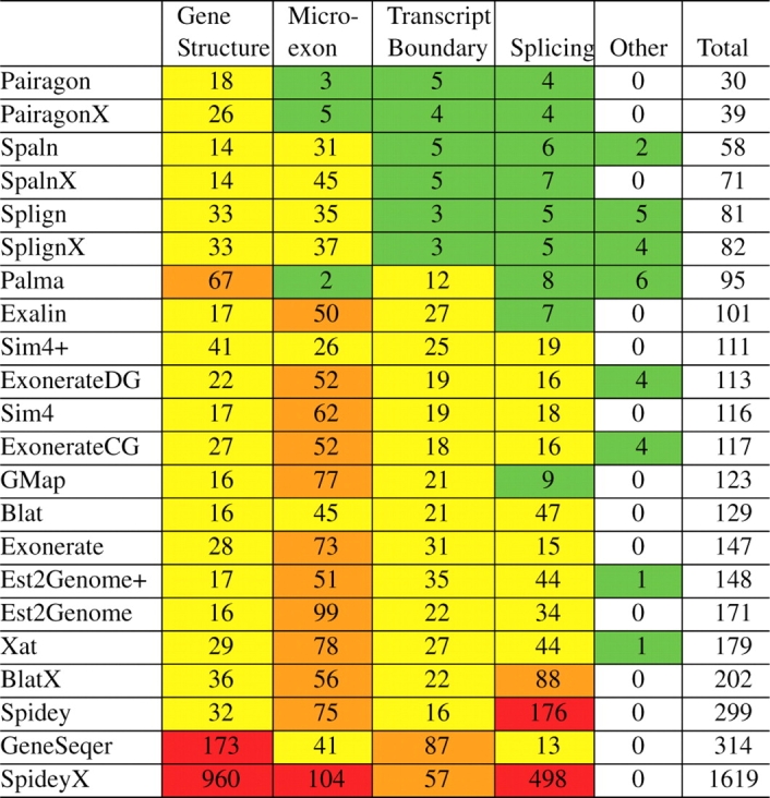Microexon errors are a subclass of the previous class (counted separately here), that involve misaligned exons that are shorter than 30 nt. Transcript boundary errors happen when either the initial or terminal exon is too long or too short at the boundary of the transcript. Splicing errors encapsulate all alignments where at least one of the splice sites is incorrect. The remaining category marks cases where the alignment was placed on the wrong strand or there was no alignment at all. Each cell in the graph shows the total number of each type of error for all of the aligners. Numbers 100 or greater are marked in red, 50 or more in orange, 10 or more in yellow and more than 0 in green.

We then decided to look more closely at the differences between the alignments output by Pairagon (because it is the most accurate) and those output by GMap (because it is very fast, widely used and generally considered to be accurate). There are 93 transcripts in which Pairagon was completely right and GMap was wrong, 5 in which GMap was completely right and Pairagon wrong, 11 in which both were equally wrong and 5 in which both made errors but Pairagon made fewer. The microexon errors made up the majority of cases in which Pairagon was completely right and GMap was not. The example shown in Figure 5a is typical: GMap left the first nine bases of the 11-base initial exon unaligned and attached the next two bases to the following exon, whereas Pairagon recognized a good pair of splice sites and put in an intron, yielding 100% identity. This illustrates the fact that Pairagon strongly penalizes leaving regions of the cDNA unaligned since the probability of transition through the unaligned cDNA state is very low. GMap will not extend the ends of the alignment if it does not increase the score under GMap's scoring system.

Fig. 5.

Alignment examples–shown here are four examples where Pairagon finds the correct alignment and GMap does not. (a) GMap adds two bases of the initial microexon to the second exon and leaves the rest unaligned. (b) GMap does not align the final base. (c) GMap incorrectly marks the left side of an intron. (d) GMap marks an insertion as an intron.

Pairagon's penalty for unaligned cDNA comes into play again in the 15 cases where the correct alignment contains a mismatch at the first or last base, as shown in Figure 5b. Note that if we were using completely natural sequences rather than a mutation simulator, we would have no way to know that these alignments with mismatches at the end were correct. In general, they might be attributed to vector sequence or some other type of error, but there is in fact no reason to think that correct mismatches are any rarer at the ends of the alignment than they are in the middle. Any aligner that fails to penalize unaligned cDNA will incorrectly omit these mismatches, shortening the exon.

Another important feature of Pairagon's scoring model, which results in a handful of correct exons missed by GMap, is its strong preference for GT splice donors over GC splice donors, reflecting their estimated frequencies in correct alignments. This is illustrated in Figure 5c, where Pairagon correctly inserts a 6-base gap to avoid two mismatches and convert a GC donor to a GT donor. As in the case of alignments ending in mismatches, there would be no way to tell which of these alignments was correct if we were not using the mutation simulator. (Indels near splice sites may have a slightly reduced frequency due to potential disruption of binding by splicing factors, however, the relatively free distribution of nucleotides in these positions suggests that such effects will be small.)

Pairagon's stronger splice site model comes into play again in the example shown in Figure 5d, along with the fact that it penalizes gap extensions less than mismatches. GMap incorrectly calls a 128-base intron with putative GG/CC splice sites, whereas Pairagon correctly calls a 128-base deletion in the genome. Both alignments have 100% identity and there would be no way to know that the genomic deletion was the correct alignment. This is a case that makes a significant difference in the exon–intron structure, but the indel polymorphism would be missed by most aligners. Indeed, cases like this in which the incorrect alignment is 100% identical to the genome may account for the small handful of very rare intron boundaries that are consistently reported (Levine and Durbin, 2001).

Given that many of the errors in alignments produced by other aligners are linked to the misalignment of microexons, we wondered whether Pairagon's advantage came primarily from an overrepresentation of microexons in our test sets. Since our test set contains cDNAs extracted from the coding regions in the annotations, a significant fraction of the microexons contained the start and stop codons, which are flanked by UTR in the full-insert cDNA sequences. The full-insert cDNA sequence have initial and terminal exons with a length distribution closer to that of internal exons. Aligning the shortened exon may seem unnatural, although it is an important case that aligners must handle, since many cDNA sequences are not 5′ complete. To investigate this question, we ran the same tests using cDNAs extracted from the full transcript, including the coding region, stop codons and 5′ and 3′ UTR. This resulted in an increase in average exon length and a decrease (but not a complete elimination) of microexons. This experiment did not substantially change the relative accuracies of the top aligners, as seen in Section 4 in Supplementary Material.

5.2 Choosing the right aligner for the job

There is an initial temptation to choose an aligner based on whether it is fast and produces alignments that ‘look good.’ Many of the aligners are considerably faster than Pairagon. GMap, sim4, Spidey, BLAT, Spaln, Splign and Xat all run each alignment in less than a second on average, where Pairagon, even with its optimizations, takes 60 s on average. See Section 5 in Supplementary Material for exact numbers. The other aligners also produce what appear to be reasonable alignments: they align most of the cDNA, have logical splice sites and a small number of mismatches and indels. Our experiments, however, allow us to discern the correct alignment, which frequently does not ‘look good.’ Figure 5b shows a correct alignment with a mismatch as the final base, which is counter-intuitive to many. Figure 5c has a large insertion near the splice site, to which manual annotators might raise objections. However, we know from our constructed reference annotation that these are the correct alignments. Clearly, one cannot tell when an alignment is correct just by looking at it (Lunter et al., 2008).

In separate experiments, we attempted to improve the speed-accuracy trade-off by running a fast aligner first, using a set of automatically computed metrics to determine whether the alignment seemed to be good, and if not, running Pairagon, which is slower but more accurate. However, none of the metrics could identify bad alignments often enough to achieve accuracy comparable to that of running Pairagon every time. The only marginally useful metric was the percent identity, which allowed us to choose either the same- or cross-species model for Pairagon. Other than that, we could not find any way to decide, on a case-by-case basis, which aligner to use. As a result, we are left with the original speed-accuracy trade-off: use the aligner whose average accuracy in a simulator is as great as possible, subject to the limits of available computing power. If you want high accuracy, such as delivered by Pairagon, for all of your alignments, you need to take the speed hit.

6 CONCLUSION

In this article, we introduced Pairagon and showed that it is an accurate alignment program for both high- and low- identity sequences. The key to its success is an intense focus on the underlying model of correct alignments, whatever the computational cost may be. By building a more realistic (and more complex!) probabilistic model of correct alignments, Pairagon is able to discern exon–intron boundaries with accuracy surpassing all other aligners we tested.

REFERENCES

- Arumugam M, et al. Pairagon+N-SCAN_EST: a model-based gene annotation pipeline. Genome Biol. 2006;7(Suppl 1):S5. doi: 10.1186/gb-2006-7-s1-s5. [DOI] [PMC free article] [PubMed] [Google Scholar]
- Florea L, et al. A computer program for aligning a cDNA sequence with a genomic DNA sequence. Genome Res. 1998;8:967. doi: 10.1101/gr.8.9.967. [DOI] [PMC free article] [PubMed] [Google Scholar]
- Gotoh O. A space-efficient and accurate method for mapping and aligning cDNA sequences onto genomic sequence. Nucleic Acids Res. 2008;36:2630. doi: 10.1093/nar/gkn105. [DOI] [PMC free article] [PubMed] [Google Scholar]
- Kapustin Y, et al. Splign: algorithms for computing spliced alignments with identification of paralogs. Biol. Direct. 2008;3:20. doi: 10.1186/1745-6150-3-20. [DOI] [PMC free article] [PubMed] [Google Scholar]
- Keibler E, et al. The treeterbi and parallel treeterbi algorithms: efficient, optimal decoding for ordinary, generalized and pair HMMs. Bioinformatics. 2007;23:545. doi: 10.1093/bioinformatics/btl659. [DOI] [PubMed] [Google Scholar]
- Kent W, et al. BLAT—the BLAST-like alignment tool. Genome Res. 2002;12:656–664. doi: 10.1101/gr.229202. [DOI] [PMC free article] [PubMed] [Google Scholar]
- Levine A, Durbin R. A computational scan for U12-dependent introns in the human genome sequence. Nucleic Acids Res. 2001;29:4006. doi: 10.1093/nar/29.19.4006. [DOI] [PMC free article] [PubMed] [Google Scholar]
- Li H, et al. A cross-species alignment tool (CAT) BMC Bioinformatics. 2007;8:349. doi: 10.1186/1471-2105-8-349. [DOI] [PMC free article] [PubMed] [Google Scholar]
- Lunter G, et al. Uncertainty in homology inferences: Assessing and improving genomic sequence alignment. Genome Res. 2008;18:298. doi: 10.1101/gr.6725608. [DOI] [PMC free article] [PubMed] [Google Scholar]
- Meyer I, Durbin R. Comparative ab initio prediction of gene structures using pair HMMs. 2002;18:1309–1318. doi: 10.1093/bioinformatics/18.10.1309. [DOI] [PubMed] [Google Scholar]
- Mott R. EST_GENOME: a program to align spliced DNA sequences to unspliced genomic DNA. 1997;13:477–478. doi: 10.1093/bioinformatics/13.4.477. [DOI] [PubMed] [Google Scholar]
- Schulze U, et al. PALMA: mRNA to genome alignments using large margin algorithms. Bioinformatics. 2007;23:1892–1900. doi: 10.1093/bioinformatics/btm275. [DOI] [PubMed] [Google Scholar]
- Slater G, Birney E. Automated generation of heuristics for biological sequence comparison. BMC Bioinformatics. 2005;6:1471–2105. doi: 10.1186/1471-2105-6-31. [DOI] [PMC free article] [PubMed] [Google Scholar]
- Usuka J, et al. Optimal spliced alignment of homologous cDNA to a genomic DNA template. Bioinformatics. 2000;16:203–211. doi: 10.1093/bioinformatics/16.3.203. [DOI] [PubMed] [Google Scholar]
- Wheelan S, et al. Spidey: a tool for mRNA-to-genomic alignments. Genome Res. 2001;11:1952. doi: 10.1101/gr.195301. [DOI] [PMC free article] [PubMed] [Google Scholar]
- Wu T, Watanabe C. GMAP: a genomic mapping and alignment program for mRNA and EST sequences. Bioinformatics. 2005;21:1859–1875. doi: 10.1093/bioinformatics/bti310. [DOI] [PubMed] [Google Scholar]
- Zhang M, Gish W. Improved spliced alignment from an information theoretic approach. Bioinformatics. 2006;22:13–20. doi: 10.1093/bioinformatics/bti748. [DOI] [PubMed] [Google Scholar]
Associated Data
This section collects any data citations, data availability statements, or supplementary materials included in this article.