

Abstract
Motivation: Reproducibility analyses of biologically relevant microarray studies have mostly focused on overlap of detected biomarkers or correlation of differential expression evidences across studies. For clinical utility, direct inter-study prediction (i.e. to establish a prediction model in one study and apply to another) for disease diagnosis or prognosis prediction is more important. Normalization plays a key role for such a task. Traditionally, sample-wise normalization has been a standard for inter-array and inter-study normalization. For gene-wise normalization, it has been implemented for intra-study or inter-study predictions in a few papers while its rationale, strategy and effect remain unexplored.
Results: In this article, we investigate the effect of gene-wise normalization in microarray inter-study prediction. Gene-specific intensity discrepancies across studies are commonly found even after proper sample-wise normalization. We explore the rationale and necessity of gene-wise normalization. We also show that the ratio of sample sizes in normal versus diseased groups can greatly affect the performance of gene-wise normalization and an analytical method is developed to adjust for the imbalanced ratio effect. Both simulation results and applications to three lung cancer and two prostate cancer data sets, considering both binary classification and survival risk predictions, showed significant and robust improvement of the new adjustment. A calibration scheme is developed to apply the ratio-adjusted gene-wise normalization for prospective clinical trials. The number of calibration samples needed is estimated from existing studies and suggested for future applications. The result has important implication to the translational research of microarray as a practical disease diagnosis and prognosis prediction tool.
Contact: ctseng@pitt.edu
Availability: http://www.biostat.pitt.edu/bioinfo/
Supplementary information: Supplementary data are available at Bioinformatics online.
1 INTRODUCTION
Microarray technology has been widely used in biomedical research, for example, in prediction of cancer diagnosis (Golub et al., 1999), of prognosis (van't Veer et al., 2002) and of treatment outcome (Shipp et al., 2002) using supervised machine-learning approaches. With an increasing amount of microarray data sets available, reproducibility analysis of these independent experiments has gained more attention and has been greatly improved in the past decade (Kuo et al., 2006; Shi et al., 2006; Tan et al., 2003; Yauk and Berndt, 2007). In the literature, most reproducibility analyses either compared and validated the detected biomarkers independently found in each study (Mitchell et al., 2004; Shi et al., 2006; Tan et al., 2003) or evaluated inter-lab or inter-platform concordance by correlation (Parmigiani et al., 2004). For direct clinical utilities, more attentions have been focused on inter-study prediction (i.e. to establish a prediction model from one data set and apply to another) recently (Shen et al., 2004; Warnat et al., 2005; Xu et al., 2008). Such an issue is critical for translating microarray technology to a practical diagnosis tool. For example, a pilot study or clinical trial has been performed in an old Affymetrix U95 platform and an effective prediction model has been constructed. The test site of another medical center may adopt another commercial system (such as Agilent or Illumina platform) or even the original medical center may have transited to a newer U133 system. The translational research of microarray would not be successful if the prediction model cannot predict inter-platform or inter-lab studies. The major difficulties for such direct inter-study prediction may include: (i) different probe design and sequence selection in different microarray platforms (Kuo et al., 2006); (ii) different sample preparation and experimental protocols; (iii) biological differences in the sample population across studies. Different data preprocessing and incorrect gene matching across studies have also been mentioned to have a great impact on such an inter-study analysis and some practical guidelines have been suggested (Bosotti et al., 2007).
Normalization is a key preprocessing step to adjust for biases in different batches within a study or in different platforms (and possibly different performance sites) across studies. In the intra-study analysis, sample-wise normalization is commonly practiced. Many mature sample-wise normalization methods have been developed and implemented, including simple standardization (standardize to zero mean and unit variance), loess normalization (Yang et al., 2002), rank-invariant normalization (Tseng et al., 2001), quantile normalization (Irizarry, et al., 2003) and median rank score (MRS; Warnat et al., 2005) (see Irizarry et al., 2006, for a comparative study). For inter-study prediction, similar sample-wise normalization methods have also been evaluated (Jiang et al., 2004; Warnat et al., 2005). To avoid the difficulty of normalization across studies, non-parametric rank-based methods have been proposed (DeConde et al., 2006; Liu et al., 2008; Xu et al., 2005). These methods, however, sacrifice information of exact intensity values and usually only simple prediction rules can be utilized. It is not clear whether the good performance can be maintained in general complex data scenarios. Another direction of efforts has been focused on statistical models for adjusting systematic microarray data biases across studies such that multiple studies may be directly pooled for analysis. Examples include singular value decomposition (SVD) (Alter et al., 2000), distance weighted discrimination (DWD) (Benito et al., 2004), cross-platform normalization (XPN) (Shabalin et al., 2008) and Knorm correlation (Teng et al., 2008). These methods involve more sophisticated modeling and have been successfully tested in some applications. The complicated models, however, have a major drawback that a larger test data set is required for parameter estimation.
Gene-wise normalization to enhance inter-study prediction has been practiced in the literature while neither its rationale nor the effectiveness has been systematically studied. It should be noted that most sample-wise normalization methods implicitly take advantage of the large number of thousands of genes to work, while for gene-wise normalization, the size of samples may only be dozens. As a result, methods like loess normalization, rank-invariant normalization and quantile normalization are not applicable to gene-wise normalization. Bloom et al. (2004) utilized a common reference sample in both training and test studies to implement gene-wise normalization while such a reference sample is generally not available. Jiang et al. (2004) performed gene-wise normalization by standardizing against the normal samples. In practice, simple standardization to zero mean and unit variance is probably most commonly used. In this article, we will discuss and elucidate the rationale for gene-wise normalization to enhance inter-study prediction. We will show that the ratios of sample sizes between normal and diseased groups can affect the performance of normalization and prediction accuracy in simple standardization. We propose a ratio-adjusted gene-wise normalization in addition to conventional sample-wise normalization. A calibration scheme is further suggested for its application to a prospective clinical trial to overcome the issue that class labels and sample size ratio are generally unknown in the population of the test study. Simulations and real data analysis of binary and survival risk prediction are used to evaluate the performance of our proposed method.
2 METHODS
2.1 Motivation
In this article, we investigate a commonly encountered situation that gene-specific discrepancies in expression intensity across studies are found in many predictive biomarkers even after proper sample-wise normalization across studies. The gene-specific discrepancies often come from different probe-sequence selections and experimental protocols that caused different gene-specific hybridization efficiencies across studies. Figure 1 in Kuo et al. (2006) demonstrated the issue that different array platforms adopt different probe designs, which caused different hybridization efficiency and bias in each platform when detecting the underlying true expression level. We further illustrate this problem in Figure 1 here. EMP2 is an ideal predictive biomarker that is down-regulated in the diseased group in the raw data (data with intra-study normalization but without inter-study normalization) of all three independent lung cancer studies (details of the data sets will be introduced in Section 2.5). The intensity values in the three studies are, however, at very different levels. Direct applications of prediction models across studies using this biomarker will perform poorly in this case. For example, applying the prediction model obtained from the Bh study to the Ga study will predict almost all subjects as adenocarcinoma patients, and the poor performance naturally calls for the need of sample normalization. In Figure 1B and C, standard normalization (std) and MRS are applied for inter-study sample-wise normalization (SN_std and SN_MRS). It is clearly seen that the expression levels of EMP2 are still not comparable across studies and that the three pairs of direct inter-study prediction (Bh versus Ga, Ga versus Be and Bh versus Be) will fail with an average accuracy rate of 73% for SN_std and 61% for SN_MRS. In Figure 1D, sample-wise and then gene-wise normalization by simple standardization to zero mean and unit variance (SN_std+GN_std) scales the expression intensities to a comparable range across three studies and an average accuracy of 94% has been reached in the three pairs of inter-study predictions, a magnitude similar to the accuracy reported in each individual paper. The result strongly argues the necessity of gene-wise normalization for a successful inter-study prediction.
Fig. 1.

example of predictive biomarker (EMP2) with gene-specific discrepancies across studies in expression intensity. (A) Raw data with intra-study normalization but without inter-study normalization. (B) Inter-study sample-wise normalization by standard normalization (SN_std). (C) Inter-study sample-wise normalization by median rank scores (SN_MRS). (D) Inter-study sample-wise normalization and then gene-wise normalization with standard normalization (SN_std+GN_std). (‘Plus’ sign denotes tumor group; ‘minus’ sign denotes normal group; means and error bars of expression intensities are scaled and represented on the y-axis.)
2.2 Simulation to demonstrate necessity of ratio adjustment
Although SN_std+GN_std In Figure 1D results in good performance, the differential sample-size ratios of normal and diseased groups among studies can potentially deteriorate the normalization and prediction. We performed two simulations below with identical ratios and with different imbalanced ratios across studies to investigate the issue. In scenario 1, we simulated a ratio-balanced univariate gene scenario for the training data and test data. Expression intensities for 100 normal samples were simulated from N(3.5, 1) and 100 tumor samples from N(6.5, 1). In the test data, we assumed that the hybridization efficiency was doubled and the expression intensities of 100 normal samples were simulated from N(7, 22) and 100 tumor samples were simulated from N(13, 22) (see Figure 3A). In scenario 2, a ratio-imbalanced scenario, the distributions remained the same but the training data contained 150 normal and 50 tumor samples while the test data contained 50 normal and 150 tumor samples. A univariate (one marker) prediction model was constructed from the training data using linear discriminant analysis (LDA) and then was evaluated in the test data. The simulation was performed 1000 times and the average error rate was reported. The prediction performance of no gene-wise normalization (Fig. 3A and B), gene-wise standard normalization (GN_std; Fig. 3C and D), ratio-adjusted gene-wise standard normalization (rGN_std; Fig. 3E and F) and the optimal Bayes error were evaluated. The Bayes error rates based on the Bayes optimal classifier given the underlying simulation model can be analytically calculated for both scenarios. Specifically, ErrorBayes(X, Y, Px, Py)=PX·∫t>λfX(t)dt+PY·∫t<λfY(t)dt where we assume E(X) < E(Y), X and Y are normal and diseased populations, fX and fY are the densities of simulated Gaussian distributions, λ is the solution of PX·fX(λ)=PY·fY(λ), and PX and PY are the proportions of normal and diseased populations in the test data. In scenario 1, PX=PY =0.5; in scenario 2, PX =0.25 and PY =0.75.
Fig. 3.

Prediction in raw and normalized data from simulation: (A) scenario1, raw data; (B) scenario2, raw data; (C) scenario1, GN_std; (D) scenario2, GN_std; (E) scenario1, rGN_std; (F) scenario2, rGN_std. Solid dots: normal samples; circles: tumor samples; solid horizontal line: prediction threshold from the training set, used to predict the test set (x-axis: index for 400 samples; y-axis: original and normalized intensity).
2.3 Ratio-adjusted gene-wise normalization
Intuitively, GN_std is sensitive to the sample ratio between normal and diseased groups in a study. We propose the following analytical approach for ratio adjustment by assuming an equal mixture model below.
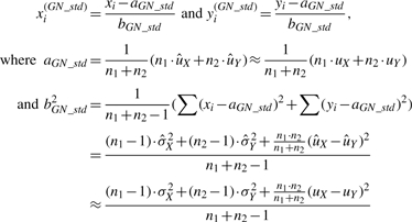
For a given gene g, we omit the subscript g and consider observed intensities (x1,…, xn1, y1,…, yn2) after sample-wise intra-study normalization, where the first n1 samples are from normal group and the next n2 samples are from diseased group. Suppose (x1,…, xn1) are i.i.d. from distribution X and (y1,…, yn2) are from Y with E(X)=uX, Var(X)=σX2, E(Y)=uY and Var(Y)=σY2. GN_std standardizes gene vector to zero mean and unit standard deviation by two parameters aGN_std and bGN_std:
 |
(1) |
where  and similarly for
  and
and  . It is clearly seen from Equation (1) that the results of GN_std greatly depend on the sample sizes n1 and n2.
We propose below a ratio-adjusted gene-wise normalization (rGN_std) method. The empirical distributions obtained from (x1,…, xn1) and (y1,…, yn2) are denoted by X′ and Y′. In other words, the cumulative distribution function (CDF) of X′ is  and, similarly,
  . Consider Z′ the equal mixture distribution of X′ and Y′ such that FZ′(t)=0.5·FX′(t)+0.5·FY′(t). Our goal is to find normalization factors arGN_std and brGN_std2 such that
  and
and  . It is easily seen that
  (uX+uY)/2 and
 |
(2) |
where, by definition,  and
and  . From Equation (2), the two ratio-adjusted scaling parameters are now invariant to n1 and n2. We note that arGN_std=aGN_std and brGN_std≈bGN_std when n1=n2. The minimum sample size required to estimate (arGN_std, brGN_std) is n1=n2=1 since the variance estimators in Equation (2) under the mixture distribution framework are MLE estimators, instead of unbiased estimators in Equation (1).
This analytic approach for ratio adjustment could be easily extended when there are more than two groups in the data. Suppose K groups are available, we can generate Z′ to be the mixture of K groups with equal weights:
The scaling parameters can be derived similarly:
2.4 Calibration scheme for prospective clinical trial
An immediate issue from rGN is that the gene-wise normalization in the test data requires knowledge of the class labels to calculate the normalization factors. This is infeasible in general prospective clinical trials. In Figure 2, we describe a calibration scheme for applying the proposed SN+rGN method to construct a prediction model from an existing training study and to perform prediction in a prospective test study (clinical trial). SN_std+rGN_std is performed in the training study and a classification model is obtained. In the prospective test study, a small set of calibration samples with known disease labels is acquired and SN_std+rGN_std is similarly applied to the calibration set to estimate the normalization factors. In practice, the calibration data set can be obtained by applying selected mRNA samples from the training study and new array data are generated using the new platform or experimental protocol in the test study. Finally, the normalization factors obtained from the calibration set and the classification model obtained from the training study are applied to all prospective test samples to predict disease status. In biological experiments, similar calibration procedures are common when the experiment is to be conducted in a new performance site or under a new protocol. An immediate advantage of using the calibration scheme with SN_std+rGN_std is that predictions can be generated sequentially whenever the test samples are collected day by day. In contrast, most sophisticated normalization methods, such as XPN, DWD and Knorm, requires the entire data matrix in test study for normalization.
Fig. 2.

Calibration scheme for predicting prospective studies.
2.5 Data sets, preprocessing and gene matching
The raw data of the three lung cancer studies: Bh (Bhattacharjee et al., 2001), Be (Beer et al., 2002) and Ga (Garber et al., 2001) were downloaded from the public Internet domain (http://www.camda.duke.edu/camda03/datasets/). Intra-study sample normalization for Bh and Be was carried out in dChip using the rank-invariant normalization. Standard normalization, which standardizes each sample to zero mean and unit variance, was applied to the cDNA data. Genes with low average intensities or small variabilities were filtered out based on the criteria developed in the original studies. Detailed information is listed in Supplementary Table 1.
For gene matching across studies, Entrez IDs were used as the common identifiers. In this article, R package ‘annotate’ was used to retrieve the Entrez IDs for the two Affymetrix data sets and MatchMiner (Bussey et al., 2003) was used for the cDNA data. Averaged values were taken for multiple probes sharing an identical Entrez ID. There were 2493 genes that overlapped in the Bh and Be data sets, 1493 genes in the Bh and Ga data sets and 1594 genes in the Be and Ga data sets. They were used for the analysis of direct inter-study prediction in this article. There were 81, 86 and 22 tumor samples, respectively, in the Bh, Be and Ga data sets with available survival follow-up information. These samples were used in the survival risk prediction analysis. We note that averaged values were used when multiple probes match to the same Entrez ID in this article. We tested two other popular approaches for the multi-probe matching issue: (i) select the probe with largest inter-quartile range (IQR); (ii) select the probe with largest Pearson correlation to the 0–1 disease phenotype vector. The results are almost identical to the averaging approach (Supplementary Fig. 1).
The two prostate cancer data sets, We (Welsh et al., 2001) in Affymetrix U95 and Dh (Dhanasekaran et al., 2001) in cDNA were publicly available. The We data set contains 9 normal and 25 cancer samples while the Dh has 19 and 14 samples, respectively. Since these two data sets were preprocessed with the Unigene ID provided, they were merged by Unigene ID. There were 3078 overlapping genes left, which were the basis of the inter-study prediction analysis used in our project.
2.6 Classification methods and evaluation
To assess the performance of our proposed normalization method regarding binary classification (the prediction of normal versus diseased samples), we examined three popular classification methods in microarray analysis: LDA, K-nearest neighbor (KNN) and prediction analysis of microarrays (PAM). For ease of evaluation, comparisons of different normalization methods were performed with identical parameters (number of genes used in LDA, PAM and KNN) and the results were verified by varying parameters over a certain range.
Overall prediction accuracy has been widely used as the evaluation index in many publications. It is, however, often a misleading measure, especially when the data set contains unbalanced sample sizes in groups. For example, the accuracy in the Be data set can be as high as 89.6% (86/96), even if the classification rule predicts all samples to be adenocarcinoma. A standard alternative to this situation may be the AUC (area under ROC curve) index by varying the classification threshold in the classification rule. This measure is, however, usually unstable for small-sample-size situations and is not readily available for classical methods like KNN. In this article, we applied a simple yet robust prediction performance index, Youden index (Youden, 1950) that is defined as:
To evaluate the risk prediction of survival, supervised principle components (SuperPC) (Bair and Tibshirani, 2004) method was used to cross predict the survival risks of the three lung cancer data sets. The coefficients of univariate Cox model fitting the expression intensities to the survival was calculated for each gene. The most significant 50 genes were kept, and singular value decomposition (SVD) was applied to select the top three principal components for fitting the Cox linear model. The risk index is defined as the linear term in the Cox model, and the median risk index value of all the training samples is used as the threshold for deciding high- or low-risk groups. Under this criterion, about half of the patients will be classified as the high-risk group and the other half will be classified as the low-risk group. We adopt two evaluation criteria in this article. For the first criterion, the performance of risk prediction is determined by the separation of survival curves of high- and low-risk groups, which is evaluated by the P-value of log-rank test comparing the two Kaplan–Meier curves from predicted high- and low-risk groups. For the second criterion, C-index (Harrel et al., 1982) that correlates the rank of predicted risk indexes and observed survival information is used.
To compare with existing methods for both binary and survival prediction, we first compare SN_std, SN_std+GN_std and SN_std+rGN_std. We then compare SN_std+rGN_std to XPN (software obtained from https://genome.unc.edu/xpn/) and DWD (software obtained from https://genome.unc.edu/pubsup/dwd/).
3 RESULTS
Figures in this section (Figs 3–7) are available in color and with higher resolution in the Supplementary Material.
Fig. 7.

Inter-study survival predictions between Be and Ga. Figure (A–E) Be => Ga. (F–J) Ga => Be. P: P-value of log-rank test. C: C-index (x-axis: survival time; y-axis: proportion of patients survived).
3.1 Simulations to validate ratio-adjusted procedure
Following the simulation model described in Section 2.2, the raw and normalized data from simulations under both scenarios are displayed In Figure 3. Comparing Figure 3C and D, GN_std normalization obtained a near optimal prediction accuracy under scenario 1 (ratio-balanced), but not under scenario 2 (ratio-imbalanced). The ratio-imbalanced situation was corrected by rGN_std (Fig. 3F). Table 1 lists the mean error rate of constructing a prediction model from the training data and predicting the test data (by LDA) using raw data, and data after applying either the GN_std or rGN_std methods based on 1000 simulations. In scenario 1, the error rates of applying GN_std and rGN_std are identical and very close to the Bayes error rate. In scenario 2, GN_std does not perform well due to the imbalanced sample ratios and applying rGN_std greatly improves GN_std.
Table 1.
Mean error rate of 1000 simulations
| Error rate | Training => Test |
|
|---|---|---|
| Scenario 1 (%) | Scenario 2 (%) | |
| Raw | 42.0 | 21.0 |
| GN_std | 6.7 | 37.5 |
| rGN_std | 6.7 | 6.6 |
| Bayes error | 6.7 | 5.5 |
3.2 Inter-study prediction in binary classification
We compared inter-study performance using raw data, as well as data normalized by the following methods: SN_std, SN_std+GN_std and SN_std+rGN_std to three lung cancer data sets: Bh, Be and Ga. The with-in study prediction in each individual study had nearly perfect performance by either SN_std or SN_std+GN_std, confirming previous reports. We tested three prediction methods: PAM, LDA and KNN. The results were slightly different but similar, so we only report PAM results In Figure 4. The results by LDA and KNN are presented in Supplementary Figures 2 and 3. Figure 4 shows Youden indexes of all three pair-wise inter-study predictions with 5, 10, 50, 100, 200 and 500 genes used in the training set. The four lines 1, 2, 3 and 4 (In Fig. 4A, C, F, G, I and K) stand for raw data, SN_std, SN_std+GN_std and SN_std+rGN_std, respectively. Without any inter-study normalization (Raw), all the inter-study predictions performed poorly with Youden Indexes around 0, which is a result of almost all the samples being predicted into one group (similar to the univariate situation In Fig. 1A). SN_std dramatically improved the inter-platform prediction between Bh and Be, two Affymetrix data sets (Fig. 4A and C). It also improved In Figure 4E and I but not In Figure 4G and K. Overall, SN_std+GN_std improved SN_std, and the results after applying SN_std+rGN_std performed the best for inter-study prediction. For example, In Figure 4G and K, SN_std+rGN_std was the only normalization method which produced satisfying inter-study prediction. We note that the gene-wise normalization in SN_std+rGN_std has utilized class label information in the test data, it poses potential risk of overfitting. However, since the class label information from test data is used only for normalization instead of for model construction, we expect the potential bias to be very minimal.
Fig. 4.

Inter-study prediction of lung cancer data by PAM. (A) and (B) Bh => Be, using Bh study as training data to predict Be study. (4C–4L) Similar notations are used for the other five inter-study predictions (x-axis: number of genes used in the prediction models; y-axis: Youden index).
We performed the same comparison for two prostate cancer studies: We and Dh (Fig. 5A and C). Inter-study predictions based on the raw data had the worst performance and all other normalization methods provided some improvement. Overall, SN_std+rGN_std has the best prediction accuracy rate and it achieves a 100% accuracy rate when in Dh => We, shown by line 4 In Figure 5C. Similar results of this inter-study evaluation by LDA and KNN are presented in Supplementary Figures 4 and 5.
Fig. 5.

Inter-study prediction of prostate cancer data by PAM. (A) and (B) We => Dh. (C) and (D) Dh => We (x-axis: number of genes used in the prediction models; y-axis: Youden index).
For a side-by-side comparison, we added XPN and DWD for comparison in the lung and prostate cancer data. In four of the six lung cancer inter-study prediction pairs (Fig. 4B, D, F and J), XPN, DWD and SN_std+rGN_std performed similarly. In the other two prediction pairs (Fig. 4H and L), DWD performed poorly and XPN slightly outperformed SN_std+rGN_std. For Dh => We prediction in prostate cancer (Fig. 5C), DWD continued to perform poorly while SN_std+GN_std outperformed XPN.
Following the calibration scheme discussed in Section 2.4 and Figure 2, we randomly selected a few samples from the test set to use as a calibration to perform SN_std+rGN_std for inter-study prediction of the three lung cancer studies. The numbers of the samples in the calibration are 1:1 (1 normal and 1 adenocarcinoma), 2:2 and 3:3 shown by line 1, 2 and 3 In Figure 6, respectively (using PAM). The prediction results were based on an average of ten random draws of calibration samples. In general, larger numbers of calibration samples provide better estimate of normalization factors. The improvement from 1:1 to 2:2 was significant while, surprisingly, not much improvement was gained from 2:2 to 3:3. The result argues that a calibration set as small as four samples (two normal and two diseased) is enough for ratio-adjusted gene-wise normalization. The same analyses are performed by using LDA and KNN, and similar results are obtained in Supplementary Figures 6 and 7. To be conservative, we suggest a calibration set of 5–6 normal and diseased samples in general when designing a serious prospective clinical trial under a different protocol, in an independent medical center or in a different array platform. Note that since the disease or survival information of the test samples is usually not available, a simple solution is to obtain biological samples from the training study and rerun the arrays in the new experimental setting to serve as the calibration set (see Fig. 2).
Fig. 6.

Inter-study predictions by SN_std+rGN_std with different number of calibration samples (x-axis: number of genes used in the prediction models; y-axis: Youden index).
3.3 Inter-study prediction in survival risk prediction
Finally, we performed inter-study prediction for patient survival risk in the three lung cancer studies. We compared raw data, and data after applying either the SN_std or SN_std+GN_std methods. We omitted the prediction based on the raw data because it performed poorly as expected. There was only slight improvement from SN_std to SN_std+GN_std in Bh versus Be and Bh versus Ga (presented in Supplementary Fig. 8). The more significant improvement happened in Be versus Ga and is shown In Figure 7. Inter-study predictions after SN_std are displayed on the first column and inter-study predictions after SN_std+GN_std are displayed on the second column. SN_std produced confusing results (Fig. 7A and F), where samples predicted as low-risk had worse survival outcomes than the high-risk group. Applying SN_std+GN_std (Fig. 7B and G), although still not statistically significant, corrected the problem and provided more reasonable predictions. Applying DWD and XPN does not improve survival prediction in Be versus Ga comparison (see Fig. 7D and I for XPN and Fig. 7E and J for DWD). In the other two comparisons (Bh versus Be and Bh versus Ga in Supplementary Fig. 8), we surprisingly found that predictions of DWD and XPN occasionally generated low-risk groups with worse survival outcomes than high-risk groups (Supplementary Fig. 8A4, B4, B5 and D4). In conclusion, even though all of the survival predictions are not statistically significant, the result supports the necessity of gene-wise normalization in addition to sample-wise normalization (SN_std+GN_std) and finds no advantage for sophisticated modeling in DWD and XPN.
It should be noted that survival risk predictions, unlike binary classification, have no known binary sample labels. The ratio-adjustment and the calibration scheme cannot be directly applied. We tested an idea of taking the three most extremely high- and low-survival samples as the calibration set (named SN_std+eGN_std; gene-wise normalization by extreme samples). The result shows similar or worse (Fig. 7C and Supplementary Fig. 8C3) performance than SN_std+GN_std without ratio adjustment. More investigations are needed for future research especially when the survival distributions of samples in two studies greatly differ.
4 DISCUSSION AND CONCLUSIONS
In this article, we investigated the normalization issue for enhancing inter-study disease prediction, a critical issue for microarray translational research. Instead of developing more sophisticated sample-wise normalization methods (SN), we observed that gene-wise discrepancies of expression levels across studies were often significant, which impeded successful inter-study prediction. As a result, the addition of gene-wise normalization (GN) is necessary. We further found that differential-sample-size ratios of diseased and normal groups greatly deteriorate the gene-wise standardization procedure. An analytical method with equal mixture assumption was proposed for ratio-adjusted gene-wise normalization (rGN). Finally, since the sample labels are needed to perform rGN, we developed a practical calibration scheme for the design of a prospective clinical trial.
Figure 1 shows that inter-study normalization is necessary before being able to perform inter-study prediction (Fig. 1A) and sample-wise normalization across studies is not sufficient to correct the bias (Fig. 1B and C). There are several potential explanations for such gene-specific intensity discrepancies. The major cause comes from the different probe designs in different array manufacturers. For example, the probes from Affymetrix GeneChip are short 25-mer oligos with multiple probes (11–16 probes) representing one gene. For cDNA microarray, the probes are cDNA fragments that are usually hundreds of bases long. As a result, probes meant to measure an identical gene always have different target sequences for hybridization in different platforms, which, in turn, introduces differential probe efficiency and affects the final intensity levels. Even if comparing studies of the same array platform, different sample preparations, as well as labeling and hybridization protocols, can possibly introduce such gene-specific intensity discrepancies.
Preprocessing by GN_std has been widely applied in gene clustering as well as particular classification methods (SVM, KNN, etc.) and dimension reduction (MDS and PCA) to obtain better scale invariant property. It is well-known that by performing GN_std, the Euclidian distance of two genes can be expressed by the correlation coefficient. In general,  where x′ and y′ are two standardized gene vectors and n is vector length. Sample-wise normalization (SN) is a routine preprocessing step in microarray analysis, while GN_std is seldom discussed in the literature. However, GN could be a critical step when dramatic gene-specific differences exist between different platforms and none of the SN methods is expected to bring the expression values to the same level for all genes. As we have shown in this article, implementation of SN+GN is fast and a significant improvement is often obtained compared to SN only. We conclude that GN should be applied in the analyses to directly carry prediction models from one study to another and ratio-adjusted GN should be used because GN is sensitive to the ratio of normal and disease groups.
To further investigate the cause of improvement in GN, we conducted a principal component analysis (PCA) on the three individual lung cancer data sets based on the top 50 genes, comparing normalization by SN_std and SN_std+GN_std. It is clearly shown in Supplementary Figure 9 that the PCA is heavily dominated by the first component after applying SN_std for all three studies. By additional GN_std, proportions of information after the second principal component are increased and can be better utilized to construct the prediction model. This explains why additional GN improves the prediction performance.
Calibration of experimental instruments is a common practice when operating in a new lab or by a new technician. It is especially necessary when preparing for a large survey or screen test. Our proposed SN_std+rGN_std method requires knowledge of sample labels in the test set and, as a result, a calibration scheme was developed for application to a prospective clinical trial. In our analysis of the three lung cancer data sets, a small calibration set of two to three normal and diseased samples respectively was sufficient. Since experimental quality and genetic variation may vary in other studies of different diseases, we conservatively suggest five to six normal and diseased samples for a serious prospective clinical trial.
Supplementary Material
ACKNOWLEDGEMENTS
The authors would like to thank the reviewers for many insightful comments to improve the manuscript.
Funding: NIH (KL2 RR024154-03); University of Pittsburgh (Central Research Development Fund, CRDF; Competitive Medical Research Fund, CMRF).
Conflict of Interest: none declared.
REFERENCES
- Alter O, et al. Singular value decomposition for genome-wide expression data processing and modeling. Proc. Natl Acad. Sci. USA. 2000;97:10101–10106. doi: 10.1073/pnas.97.18.10101. [DOI] [PMC free article] [PubMed] [Google Scholar]
- Bair E, Tibshirani R. Semi-supervised methods to predict patient survival from gene expression data. PLoS Biol. 2004;2:E108. doi: 10.1371/journal.pbio.0020108. [DOI] [PMC free article] [PubMed] [Google Scholar]
- Beer DG, et al. Gene-expression profiles predict survival of patients with lung adenocarcinoma. Nat. Med. 2002;8:816–824. doi: 10.1038/nm733. [DOI] [PubMed] [Google Scholar]
- Benito M, et al. Adjustment of systematic microarray data biases. Bioinformatics. 2004;20:105–114. doi: 10.1093/bioinformatics/btg385. [DOI] [PubMed] [Google Scholar]
- Bhattacharjee A, et al. Classification of human lung carcinomas by mRNA expression profiling reveals distinct adenocarcinoma subclasses. Proc. Natl Acad. Sci. USA. 2001;98:13790–13795. doi: 10.1073/pnas.191502998. [DOI] [PMC free article] [PubMed] [Google Scholar]
- Bloom G, et al. Multi-platform, multi-site, microarray-based human tumor classification. Am. J. Pathol. 2004;164:9–16. doi: 10.1016/S0002-9440(10)63090-8. [DOI] [PMC free article] [PubMed] [Google Scholar]
- Bosotti R, et al. Cross platform microarray analysis for robust identification of differentially expressed genes. BMC Bioinformatics. 2007;8(Suppl. 1):S5. doi: 10.1186/1471-2105-8-S1-S5. [DOI] [PMC free article] [PubMed] [Google Scholar]
- Bussey KJ, et al. MatchMiner: a tool for batch navigation among gene and gene product identifiers. Genome Biol. 2003;4:R27. doi: 10.1186/gb-2003-4-4-r27. [DOI] [PMC free article] [PubMed] [Google Scholar]
- DeConde RP, et al. Combining results of microarray experiments: a rank aggregation approach. Stat. Appl. Genet. Mol. Biol. 2006;5 doi: 10.2202/1544-6115.1204. Article 15. [DOI] [PubMed] [Google Scholar]
- Dhanasekaran SM, et al. Delineation of prognostic biomarkers in prostate cancer. Nature. 2001;412:822–826. doi: 10.1038/35090585. [DOI] [PubMed] [Google Scholar]
- Garber ME, et al. Diversity of gene expression in adenocarcinoma of the lung. Proc. Natl Acad. Sci. USA. 2001;98:13784–13789. doi: 10.1073/pnas.241500798. [DOI] [PMC free article] [PubMed] [Google Scholar]
- Golub TR, et al. Molecular classification of cancer: class discovery and class prediction by gene expression monitoring. Science. 1999;286:531–537. doi: 10.1126/science.286.5439.531. [DOI] [PubMed] [Google Scholar]
- Harrel FE, et al. Evaluating the yield of medical tests. JAMA. 1982;247:2543–2546. [PubMed] [Google Scholar]
- Irizarry RA, et al. Summaries of Affymetrix GeneChip probe level data. Nucleic Acids Res. 2003;31:e15. doi: 10.1093/nar/gng015. [DOI] [PMC free article] [PubMed] [Google Scholar]
- Irizarry RA, et al. Comparison of Affymetrix GeneChip expression measures. Bioinformatics. 2006;22:789–794. doi: 10.1093/bioinformatics/btk046. [DOI] [PubMed] [Google Scholar]
- Jiang H, et al. Joint analysis of two microarray gene-expression data sets to select lung adenocarcinoma marker genes. BMC Bioinformatics. 2004;5:81. doi: 10.1186/1471-2105-5-81. [DOI] [PMC free article] [PubMed] [Google Scholar]
- Kuo WP, et al. A sequence-oriented comparison of gene expression measurements across different hybridization-based technologies. Nat. Biotechnol. 2006;24:832–840. doi: 10.1038/nbt1217. [DOI] [PubMed] [Google Scholar]
- Liu HC, et al. Cross-generation and cross-laboratory predictions of Affymetrix microarrays by rank-based methods. J. Biomed. Inform. 2008;41:570–579. doi: 10.1016/j.jbi.2007.11.005. [DOI] [PubMed] [Google Scholar]
- Mitchell SA, et al. Inter-platform comparability of microarrays in acute lymphoblastic leukemia. BMC Genomics. 2004;5:71. doi: 10.1186/1471-2164-5-71. [DOI] [PMC free article] [PubMed] [Google Scholar]
- Parmigiani G, et al. A cross-study comparison of gene expression studies for the molecular classification of lung cancer. Clin. Cancer. Res. 2004;10:2922–2927. doi: 10.1158/1078-0432.ccr-03-0490. [DOI] [PubMed] [Google Scholar]
- Shabalin AA, et al. Merging two gene-expression studies via cross-platform normalization. Bioinformatics. 2008;24:1154–1160. doi: 10.1093/bioinformatics/btn083. [DOI] [PubMed] [Google Scholar]
- Shen R, et al. Prognostic meta-signature of breast cancer developed by two-stage mixture modeling of microarray data. BMC Genomics. 2004;5:94. doi: 10.1186/1471-2164-5-94. [DOI] [PMC free article] [PubMed] [Google Scholar]
- Shi L, et al. The MicroArray Quality Control (MAQC) project shows inter- and intraplatform reproducibility of gene expression measurements. Nat. Biotechnol. 2006;24:1151–1161. doi: 10.1038/nbt1239. [DOI] [PMC free article] [PubMed] [Google Scholar]
- Shipp MA, et al. Diffuse large B-cell lymphoma outcome prediction by gene-expression profiling and supervised machine learning. Nat. Med. 2002;8:68–74. doi: 10.1038/nm0102-68. [DOI] [PubMed] [Google Scholar]
- Tan PK, et al. Evaluation of gene expression measurements from commercial microarray platforms. Nucleic Acids Res. 2003;31:5676–5684. doi: 10.1093/nar/gkg763. [DOI] [PMC free article] [PubMed] [Google Scholar]
- Teng SL, et al. A statistical framework to infer functional gene associations from multiple biologically interrelated microarray experiments. J. Am. Stat. Assoc. 2008 (in press) [Google Scholar]
- Tseng GC, et al. Issues in cDNA microarray analysis: quality filtering, channel normalization, models of variations and assessment of gene effects. Nucleic Acids Res. 2001;29:2549–2557. doi: 10.1093/nar/29.12.2549. [DOI] [PMC free article] [PubMed] [Google Scholar]
- van't Veer LJ, et al. Gene expression profiling predicts clinical outcome of breast cancer. Nature. 2002;415:530–536. doi: 10.1038/415530a. [DOI] [PubMed] [Google Scholar]
- Warnat P, et al. Cross-platform analysis of cancer microarray data improves gene expression based classification of phenotypes. BMC Bioinformatics. 2005;6:265. doi: 10.1186/1471-2105-6-265. [DOI] [PMC free article] [PubMed] [Google Scholar]
- Welsh JB, et al. Analysis of gene expression identifies candidate markers and pharmacological targets in prostate cancer. Cancer Res. 2001;61:5974–5978. [PubMed] [Google Scholar]
- Xu L, et al. Robust prostate cancer marker genes emerge from direct integration of inter-study microarray data. Bioinformatics. 2005;21:3905–3911. doi: 10.1093/bioinformatics/bti647. [DOI] [PubMed] [Google Scholar]
- Xu L, et al. Merging microarray data from separate breast cancer studies provides a robust prognostic test. BMC Bioinformatics. 2008;9:125. doi: 10.1186/1471-2105-9-125. [DOI] [PMC free article] [PubMed] [Google Scholar]
- Yang YH, et al. Normalization for cDNA microarray data: a robust composite method addressing single and multiple slide systematic variation. Nucleic Acids Res. 2002;30:e15. doi: 10.1093/nar/30.4.e15. [DOI] [PMC free article] [PubMed] [Google Scholar]
- Yauk CL, Berndt ML. Review of the literature examining the correlation among DNA microarray technologies. Environ. Mol. Mutagen. 2007;48:380–394. doi: 10.1002/em.20290. [DOI] [PMC free article] [PubMed] [Google Scholar]
- Youden WJ. Index for rating diagnostic tests. Cancer. 1950;3:32–35. doi: 10.1002/1097-0142(1950)3:1<32::aid-cncr2820030106>3.0.co;2-3. [DOI] [PubMed] [Google Scholar]
Associated Data
This section collects any data citations, data availability statements, or supplementary materials included in this article.