Sensitivity Analysis Using Elicited Expert Information for Inference With Coarsened Data: Illustration of Censored Discrete Event Times in the AIDS Link to Intravenous Experience (ALIVE) Study

Abstract

In this paper, the authors use the rubric of “coarsened data,” of which missing and censored data are special cases, to motivate the elicitation and use of expert information for performing sensitivity analyses of censored event-time data. Elicited information is important because observed data are insufficient to estimate how study participants with coarsened data compare with participants with uncoarsened data, and misspecifying this comparison may produce biased analysis results. In the presence of coarsening, performing a sensitivity analysis over a range of plausible assumptions is the best one can do. Here the authors illustrate an approach for eliciting expert information for use in sensitivity analyses to compare cumulative incidence functions of censored nonmortality outcomes. An example of such data is the AIDS Link to Intravenous Experience (ALIVE) Study, where the authors aim to estimate and compare cumulative incidence functions for human immunodeficiency virus between risk factor categories. The interval and right-censoring and censoring due to death found in the ALIVE data (1988–1998) are thought to be informative; thus, a sensitivity analysis is performed using information elicited from 2 ALIVE scientists and an expert in acquired immunodeficiency syndrome epidemiology about the relation between seroconversion and censoring.

Incomplete data, including missing and censored data, are common challenges in epidemiology.

The main challenge is that selection bias can result from inability to determine how participants with complete and incomplete data differ. For missing data, statistical methods facilitating sensitivity analysis have been developed (1) and advocated (2). These methods involve performing analysis over ranges of plausible yet untestable assumptions about the missingness mechanism (relation between participant characteristics and probability of missingness). Sensitivity analysis using elicited expert information is recommended because subject-matter experts can posit scientifically plausible assumptions (2).

Despite available statistical methods, missing data are often inadequately addressed (3). Typically “complete case” analyses are performed that delete observations with missing variables, which may produce bias unless data are missing completely at random (4) (i.e., there is an equal probability of missingness for all participants). Sensitivity analysis is rarely performed and is often limited to imputing extreme or other scientifically implausible values, which almost always produces inconclusive results (3).

Missingness is 1 member of a broader class of incomplete-data structures called coarsening. Coarsening occurs when some set of values containing the exact value is observed, but not the exact value itself (5, 6). Other than missing data (where the set contains all possible values of the variable), coarsening includes censoring, grouping, and rounding as special cases. Conceptualizing incomplete data under the rubric of coarsening is beneficial for generalizing methods for missing data to other incomplete-data problems. Concern centers around inability to estimate the coarsening mechanism (relation between participant characteristics and probability of being coarsened into a set) and bias resulting from incorrect assumptions about coarsening.

In this paper, we illustrate the elicitation and use of expert information about coarsening for frequentist and Bayesian sensitivity analyses of interval-censored data. We use data from the AIDS Link to Intravenous Experience (ALIVE) Study, a prospective study with censored times to human immunodeficiency virus (HIV) infection and censoring by death.

EXAMPLE: THE ALIVE STUDY

Begun in 1988, ALIVE is a prospective observational study of risk factors for HIV infection among injection drug users in Baltimore, Maryland. Seronegative participants were recruited through community outreach and were interviewed regarding potential risk factors (7–9). Determination of HIV serostatus, a proxy for infection status, was scheduled through semiannual laboratory blood tests using enzyme-linked immunosorbent assay confirmed by Western blot. The estimated sensitivity and specificity of ALIVE data are over 99% (10); therefore, misclassification is not addressed here.

We operationalize infection time here as year of seroconversion. ALIVE participants often miss study visits or attend off-schedule visits, sometimes producing interval-censored seroconversion times that are known only within a range of years (i.e., an unknown, untestable coarsening mechanism that may produce bias if incorrectly modeled). Discretizing time introduces noninformative coarsening (a known mechanism) (5, 6), provides clinically interpretable results, reduces sensitivity to small departures from the visit schedule (visits within the year scheduled are considered uncoarsened here, but visits more than a year off schedule can lead to coarsening), and circumvents mathematical difficulties related to continuous interval-censoring (11). Some seroconversion times are right-censored by withdrawal, administrative censoring, or death. In this paper, we estimate and compare 10-year cumulative incidence functions (1988–1998) of seroconversion between participants who self-reported sharing needles for drug injection upon enrollment and participants who self-reported not sharing needles upon enrollment. Time-varying needle-sharing is unaddressed here; the development of methods utilizing it is planned for future research.

Among 2,205 ALIVE participants, 1,527 reported sharing needles and 678 did not. Of needle-sharers’ seroconversion times (years), 12%, 74%, 9%, and 4% were censored by death, censored by dropout or administrative censoring, interval-censored, and exactly observed, respectively. Respective percentages among nonsharers were 11, 77, 8, and 4.

Although censoring class percentages are similar between needle-sharers and nonsharers, observed data alone cannot determine how censoring and seroconversion relate. Therefore, analysis requires unverifiable assumptions about censoring. To tackle this problem, we elicit information from 2 ALIVE investigators (N. G., D. V.) and an expert in acquired immunodeficiency syndrome epidemiology for performing frequentist and Bayesian sensitivity analyses to estimate and compare needle-sharing specific incidence functions (12, 13). Before discussing statistical models, we describe the data structure and formalize the concept of coarsening.

DATA STRUCTURE

To accommodate assumptions about coarsening in statistical models, 2 types of variables are needed: the coarsened variable (in ALIVE, seroconversion time) and coarsening process variables (in ALIVE, censoring variables). For missing data, a response indicator (yes/no) describes the coarsening process. Additional notation is unnecessary because missingness does not restrict possible values for the coarsened variable.

In ALIVE, the potentially coarsened variable is T_i, year of seroconversion (from enrollment) for participant i. For an M-year study, T_i = t denotes seroconversion during year t, where t can be 1, 2, …, M − 1, M. If participant i did not seroconvert within M years, we arbitrarily set T_i = M + 1 (12).

To denote coarsening, L_i and R_i, respectively, are the earliest and latest possible years of seroconversion induced by censoring. They are the left and right endpoints of random interval [L_i, R_i], into which T_i is coarsened. For example, if participant i is last observed as seronegative during year 2 and is first observed as seropositive during year 5, then T_i is coarsened into interval [L_i = 2, R_i = 5] and T_i ∈ [2, 5]. However, if participant i is observed as seronegative during year 2 but never returns, then R_i = M + 1. Therefore, T_i ∈ [2, M + 1]; seroconversion may occur anytime after withdrawal. If participant i is observed as seronegative during year 2 and tests positive later during year 2, then L_i = 2, R_i = 2, and T_i = 2. If participant i is observed as seronegative at the end of year M (final study year), then L_i = R_i = M + 1; thus, T_i = M + 1.

While some participants may miss visits by choice, others may die during the study. Censoring by death affects possible seroconversion times. For example, if participant i is last observed as seronegative during year 2 and dies during year 5, then serostatus at death is unknown. Thus, possible seroconversion times are [2, 5] and M + 1. Let Δ_i = 1 if T_i is censored by death, and Δ_i = 0 otherwise. Having Δ_i = 1 implies that R_i is not the first year of observed seropositivity but rather is the latest possible year of seroconversion. Thus, L_i = 2, R_i = 5, and Δ_i = 1 imply T_i ∈ {[2, 5], M + 1}, whereas L_i = 2, R_i = 5, and Δ_i = 0 imply T_i ∈ [2, 5]. When a participant's vital status is unknown, R_i = M + 1, because no available information excludes times after L_i. We only consider death in order to specify the censoring set, not as a primary outcome. We are interested in estimating the cumulative incidence of seroconversion. Thus, in our approach, we specify participants as no longer being at risk of seroconversion after death (14–16).

We focus on comparing cumulative HIV incidence functions between 2 groups. Let g = s denote needle-sharers and g = n denote nonsharers, where subscript g denotes group-specific quantities (e.g., incidence).

COARSENING MECHANISMS

We formally define coarsening at random (CAR) and coarsening not at random (CNAR). For clarification, we first relate these concepts to missing data and then focus on censoring.

Coarsening at random

CAR means that the coarsened variable (e.g., study outcome) and the coarsening process are independent, given the set of values into which the variable is coarsened. With abuse of notation, CAR means

or

where “coarsening” refers to coarsening process variables, “outcome” refers to the outcome variable, and “set” refers to the set of values into which the outcome is coarsened. Let Y denote a potentially missing outcome. Missingness does not exclude possible values for Y; thus, CAR means P(missing|Y) = P(missing) or P(Y|missing) = P(Y), the well-known definition of data missing at random (4) when other relevant fully observed variables are unavailable. Thus, data being missing at random is a special case of CAR (17).

For ALIVE, CAR means that seroconversion is independent of censoring, given possible seroconversion times induced by censoring. For participants in group g = n, s not censored by death, CAR means

(1)

Similarly, for those censored by death in group g, CAR is

(2)

Equations 1 and 2 are selection models that describe how T affects the probability of being “selected” into interval [L, R] (18). Let p_gt denote the probability of seroconverting during year t among group g participants. CAR can be represented using pattern-mixture models (models describing how the coarsening “pattern,” L and R, affects the distribution of T) (19, 20):

(3)

for participants in group g = n, s, and δ = 0, 1. When assuming CAR, $p_{g1},\dots ,p_{g(M+1)}$ are estimated using Turnbull's method (21).

Models for CNAR

For missing data, several statistical methods have been proposed assuming that data are missing not at random (i.e., the potentially missing variable affects the probability of missingness). Methods exist for both selection models (22) and pattern-mixture models (2, 19, 20).

Pattern-mixture models were proposed to “tilt” the outcome distribution toward stochastically (i.e., on average) higher or lower values relative to that assumed under CAR, based on functions of inestimable elicited parameters (23). This idea was extended to interval-censored data (12). In ALIVE, censoring bias functions (12) specify whether experts believe seroconversion occurs stochastically earlier or later within the coarsening set, relative to that assumed under CAR. Let q_g(t) denote a generic censoring bias function. We use pattern-mixture models to accommodate q_g(t):

(4)

The left-hand sides of equations 3 and 4 are equivalent, because L = l, R = r, Δ = δ specifies the possible seroconversion times.

To understand q_g(t), consider needle-sharers (g = s) with L = 2, R = 5, and Δ = 0, where p_s2 = 0.1, p_s3 = 0.15, p_s4 = 0.15, and p_s5 = 0.2. Assuming CAR, equation 3 for t = 2 equals

For t = 3, 4, and 5, equation 3 equals 0.25, 0.25, and 0.33, respectively. Assuming CNAR with censoring bias function q_s(t) = ϕ_s × (t − l) and ϕ_s = 0.1, equation 4 for t = 2 equals

For t = 3, 4, and 5, equation 4 equals 0.23, 0.25, and 0.38, respectively. If, however, ϕ_s = −0.1, then for t = 2, equation 4 equals 0.20, and for t = 3, 4, and 5, it equals 0.27, 0.24, and 0.29, respectively. In the former CNAR example, seroconversion is assumed to occur stochastically later in comparison with CAR; in the latter, seroconversion is assumed to occur stochastically earlier relative to CAR. Thus, q_s(t) can “tilt” the seroconversion distribution toward later or earlier times, depending on ϕ_s.

Selection models are useful for interpreting q_g(t). Let t_ref denote some reference time where q_g(t_ref) = 0. For q_s(t) = ϕ_s × (t − l), t_ref = l. Using Bayes’ theorem, it can be shown (12) that

(5)

Thus, exp{q_g(t)} is the probability ratio of L = l, R = r, Δ = δ, comparing participants who seroconverted during year t with those who seroconverted during year t_ref. If q_g(t) is constant in t, equation 4 simplifies to equation 3, and CAR is assumed.

Parameterization of q_g(t) for ALIVE

For sensitivity analysis, q_g(t) should be parsimoniously specified yet capture key study features. For q_g(t) to be interpretable, it should be specified so that t_ref is included in [l, r]. The example ϕ_g × (t − l) adheres to this guideline, because t_ref = l. Using too many parameters results in unwieldy sensitivity analyses, while using too few parameters is overly simplistic. Because q_g(t) cannot be estimated from data, no empirical diagnostic can assess its fit; therefore, input from subject-matter experts is essential.

For ALIVE, we specify 3 classes of coarsening patterns: interval censoring (class 1), right-censoring (class 2), and death (class 3). It was thought plausible that participants in different classes would have different coarsening mechanisms and that the mechanism would depend on censoring endpoints (l and r) and needle-sharing status. To capture these characteristics in a scientifically interpretable manner that facilitates elicitation and maintains parsimony, we propose the following censoring bias function:

(6)

where ϕ (vector of scalars ϕ_gc; g = n, s; c = 1, 2, 3) are called censoring bias parameters (12) for group g and coarsening class c; and I(·) denotes the indicator function. From equations 5 and 6,

• exp{ϕ_g1} is the needle-sharing-specific probability ratio of having censoring interval [1 year, 5 years] comparing persons seroconverting during year 5 with persons seroconverting during year 1;

• exp{ϕ_g2} is the needle-sharing-specific probability ratio of dropping out after baseline comparing persons not seroconverting within 10 years with persons seroconverting during year 1, among those remaining alive throughout the study; and

• exp{ϕ_g3} is the needle-sharing-specific probability ratio of dropping out after baseline comparing persons not seroconverting while alive with persons seroconverting during year 1, among those dying during the study.

The factor 9/4 in equation 6 accounts for 10-year follow-up, but investigators preferred stating beliefs for 5-year intervals. When exp{ϕ_gc} > 1, participants in censoring class c are assumed to seroconvert stochastically later in comparison with CAR. Similarly, when exp{ϕ_gc} < 1, participants in censoring class c are assumed to seroconvert stochastically earlier in comparison with CAR.

ELICITING EXPERT INFORMATION

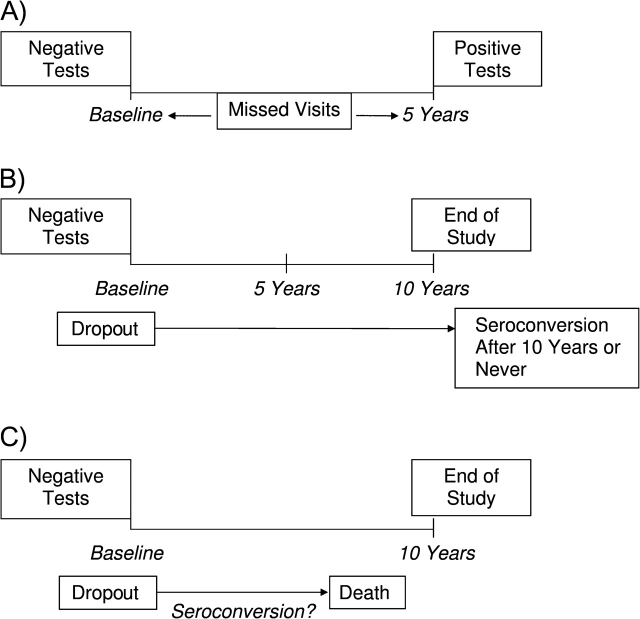
Censoring bias parameters are not estimable without additional assumptions (ideally elicited from subject-matter experts) (24–26). We elicited information from 2 ALIVE investigators and 1 external acquired immunodeficiency syndrome epidemiologist. For elicitation of ϕ in equation 6, 2 ALIVE investigators (D. V., N. G.) were separately shown Figure 1 and were asked 3 pairs of questions: 1) “Among those who self-reported needle-sharing at baseline, who was more likely to test negative for HIV at baseline, miss visits, then return during the fifth year and test positive: one who seroconverted during the first year or one who seroconverted during the fifth year? How many times more likely?”; 2) “Among those who self-reported needle-sharing at baseline and who remained alive throughout the study, who was more likely to test negative for HIV at baseline, then drop out: one who seroconverted during the first year or one who did not seroconvert within 10 years? How many times more likely?”; and 3) “Among those who self-reported needle-sharing at baseline, who was more likely to test negative for HIV at baseline, then drop out and die with unknown serostatus: one who seroconverted during the first year, or one who did not seroconvert while at risk? How many times more likely?” The questions were repeated for nonsharers.

Figure 1.

Schematic for elicitation of the coarsening mechanism among participants in the AIDS Link to Intravenous Experience (ALIVE) Study, Baltimore, Maryland, 1988–1998. A, interval-censored participants in ALIVE; B, right-censored participants in ALIVE who are not censored by death; C, right-censored participants in ALIVE who are censored by death.

Elicited $\exp \left\{\mathbf{\text{ϕ}}\right\}$ varied between investigators. A consensus was reached (Table 1, columns 4 and 5) by experts agreeing to connect their elicited ranges. The experts believed that needle-sharers who seroconverted during year 5 were 1.75 times less likely to 2.75 times more likely to be censored into interval [1 year, 5 years] than needle-sharers who seroconverted within 1 year. The range for nonsharers was 1.15 times less likely to 2.50 times more likely. Experts expressed uncertainty about this relation's direction, because some early seroconverters may return later as health diminishes, while others may return early for treatment to slow disease progression. For participants who were alive after 10 years, the experts believed that needle-sharers not seroconverting within 10 years were 1.50–3.00 times more likely to drop out after baseline than needle-sharers who seroconverted within 1 year. Among nonsharers, the range was 1.75–2.50 times more likely. Participants who are seronegative after 10 years probably engage in fewer high-risk behaviors than early seroconverters, providing little benefit in study participation and increasing the likelihood of dropping out. The experts believed that nonseroconverters who died within 10 years were 2.00–2.50 times more likely to drop out than participants who seroconverted within 1 year with the same needle-sharing status, because early seroconverters are expected to attend study visits as their health worsens.

Table 1.

Elicited Range of $\exp \left\{\mathbf{\text{ϕ}}\right\}$ and Parameters for β Distributions Used in Bayesian Analyses

Needle-Sharing	Censoring	ϕ	Range of exp{ϕ}		Shape	Scale
			Minimum	Maximum
Yes	Interval-censored	ϕs1	1.75−1	2.75	2.00	7.75
	Dropped out	ϕs2	1.50	3.00	5.25	2.75
	Deceased	ϕs3	2.00	2.50	2.00	1.00
No	Interval-censored	ϕn1	1.15−1	2.50	2.00	9.50
	Dropped out	ϕn2	1.75	2.50	3.75	2.00
	Deceased	ϕn3	2.00	2.50	2.00	1.00

Prior distributions of p_gt and ϕ for Bayesian analyses were elicited from an acquired immunodeficiency syndrome epidemiologist and an ALIVE investigator, respectively. An expert unaffiliated with ALIVE was chosen for opinions prior to knowledge gained from the ALIVE Study. HIV incidence depends on population seroprevalence (27). Given Baltimore's high 1988 HIV seroprevalence (24%) among injection drug users (7) and HIV prevention efforts (28), the elicited prior 10-year cumulative incidence was 35%; using Dirichlet priors (12), this prior incidence was weighted 10% of the final results (ALIVE data weighted 90%), indicating prior uncertainty. This uncertainty means that ALIVE data more strongly influence results than does the prior. Prior information about incidence was not needle-sharing-specific to reflect the “null” belief of equality.

Prior distributions for ϕ were obtained by displaying histograms of data generated from several β distributions for each ϕ_gc to an ALIVE investigator (D. V.). Data were centered and scaled to reflect elicited ranges of $\text{exp}\left\{\mathbf{\text{ϕ}}\right\}$ to graphically elicit β parameters. The elicited prior distributions and β parameters are shown in Figure 2 and Table 1 (columns 6 and 7), respectively.

Figure 2.

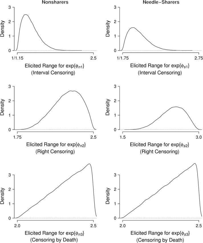
Elicited prior exp{ϕ} β densities, given elicited ranges (x-axis), AIDS Link to Intravenous Experience (ALIVE) Study, Baltimore, Maryland, 1988–1998.

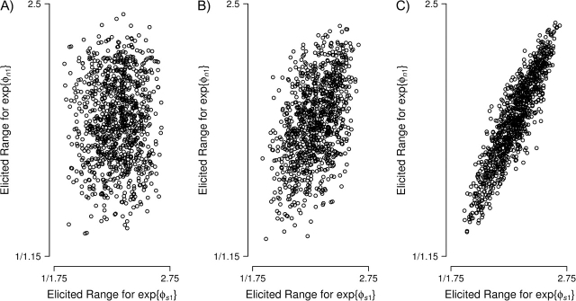
To specify the multivariate prior distribution of ϕ, we elicited pairwise correlations for ϕ_gc. We displayed to the ALIVE investigator scatterplots like those in Figure 3 (multivariate normal approximation to the β distribution) depicting pairwise correlations between parameters. The investigator's prior correlation matrix,

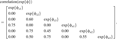indicates high correlations between needle-sharing groups within censoring class, reflecting believed similarity within censoring types regarding other HIV risk factors (e.g., sexual behavior). High correlations within right-censored status (c = 2, 3) reflect the belief that many persons dying with an unknown serostatus may not have returned to the study even if they had remained alive during follow-up. Beliefs about interval-censored event times (c = 1) were uncorrelated with those regarding right-censored event times (c = 2, 3), because motivations for visit compliance may differ.

Figure 3.

Elicitation figure for prior pairwise correlation between exp{ϕ_n1} and exp{ϕ_s1}, AIDS Link to Intravenous Experience (ALIVE) Study, Baltimore, Maryland, 1988–1998. A) correlation = 0; B) correlation = 0.5; C) correlation = 0.9.

ESTIMATION AND INFERENCE

We briefly describe methods for estimating p_gt in model 4 using equation 6 and comparing cumulative incidence functions between needle-sharers and nonsharers. For frequentist estimation, we adapt the method of Shardell et al. (12), which simplifies to Turnbull's (21) method when assuming CAR. Censored times are replaced by expected values (equation 4) using the expectation-maximization algorithm (29) described by Shardell et al. (12). Estimates are used to perform the log-rank-type test (13).

Bayesian estimation is performed for fixed and random ϕ via the Gibbs sampler (30) in the paper by Shardell et al. (12). A posterior parameter distribution (distribution conditional on observed data) motivated by the log-rank test is calculated and compared with a standard normal distribution, the expected distribution under the null hypothesis of equal cumulative incidence functions. Similarity between observed and expected posterior distributions is summarized by a tail probability. Tail probabilities of 0 and 1 correspond to no distributional overlap and perfect distributional overlap, respectively. The tail probability quantifies how rare the parameter values corresponding to the null hypothesis are under their posterior distribution, as described by Shardell et al. (13).

For both frequentist and fixed-ϕ Bayesian estimation of ALIVE, we perform sensitivity analysis under 3 assumptions: CAR ($\mathbf{\text{ϕ}}=0$), maximum elicited ${\mathbf{\text{ϕ}}}_n$ values with minimum elicited ${\mathbf{\text{ϕ}}}_s$ values, and vice versa, where ${\mathbf{\text{ϕ}}}_g$ denotes the parameter vector for group g = n, s.

ALIVE SENSITIVITY ANALYSIS RESULTS

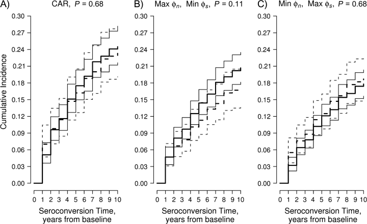
Figure 4 shows results from frequentist analysis. When needle-sharers and nonsharers are assumed to seroconvert stochastically late and early, respectively—that is, {max(${\mathbf{\text{ϕ}}}_s$), min(${\mathbf{\text{ϕ}}}_n$)}—estimated 10-year incidences for needle-sharers and nonsharers are 0.21 (95% confidence interval (CI): 0.18, 0.24) and 0.17 (95% CI: 0.14, 0.21), respectively (P = 0.11). For the opposite assumption, {min(${\mathbf{\text{ϕ}}}_s$), max(${\mathbf{\text{ϕ}}}_n$)}, estimated 10-year incidences for needle-sharers and nonsharers are 0.18 (95% CI: 0.16, 0.20) and 0.19 (95% CI: 0.15, 0.23), respectively (P = 0.68). These assumptions produce lower estimated 10-year cumulative incidences than assuming CAR (needle-sharers: 0.24 (95% CI: 0.22, 0.28); nonsharers: 0.23 (95% CI: 0.19, 0.28)), owing to $\text{min}\left(\exp \left\{{\text{ϕ}}_{gc}\right\}\right)>1$ for dropouts (c = 2, 3), the largest censoring classes in ALIVE.

Figure 4.

Frequentist results for the AIDS Link to Intravenous Experience (ALIVE) Study, Baltimore, Maryland, 1988–1998. Depicted across the range of elicited assumptions are the log-rank P value and the cumulative incidences for needle-sharers (—) and nonsharers (– – –) and their 95% confidence intervals (— and - - -, respectively). CAR, coarsening at random; Max, maximum; Min, minimum.

Figure 5 shows results from Bayesian analysis. Fixed-ϕ analyses were run for 5,000 iterations with 500 burn-in iterations; random-ϕ analysis was run for 10,000 iterations with 1,000 burn-in iterations. A diagnostic scheme including trace plots for parameters simulated from 2 parallel chains, autocorrelation functions of each parameter, and cross-correlation functions (31) suggested Markov chain convergence. Mean posterior cumulative incidences were higher than analogous frequentist estimates, because prior 10-year incidence (35%) was higher than frequentist estimates. When needle-sharers and nonsharers were assumed to seroconvert stochastically late and early, respectively, {max(${\mathbf{\text{ϕ}}}_s$), min(${\mathbf{\text{ϕ}}}_n$)}, posterior mean 10-year incidences for needle-sharers and nonsharers were 0.23 (95% credible interval (CrI): 0.20, 0.26) and 0.20 (95% CrI: 0.16, 0.23), respectively (tail probability = 0.12). When making the opposite assumption, {min(${\mathbf{\text{ϕ}}}_s$), max(${\mathbf{\text{ϕ}}}_n$)}, posterior mean 10-year incidences for needle-sharers and nonsharers were 0.20 (95% CrI: 0.18, 0.22) and 0.21 (95% CrI: 0.18, 0.25), respectively (tail probability = 0.63). Random-ϕ Bayesian analyses produced intermediate estimates (needle-sharers: 0.21 (95% CrI: 0.18, 0.23); nonsharers: 0.20 (95% CrI: 0.17, 0.24); tail probability = 0.74). Corresponding closely with frequentist results (because of the high weight given to ALIVE data), mean posterior 10-year cumulative incidences were larger assuming CAR than assuming elicited ranges (needle-sharers: 0.26 (95% CrI: 0.24, 0.29); nonsharers: 0.26 (95% CrI: 0.22, 0.30)).

Figure 5.

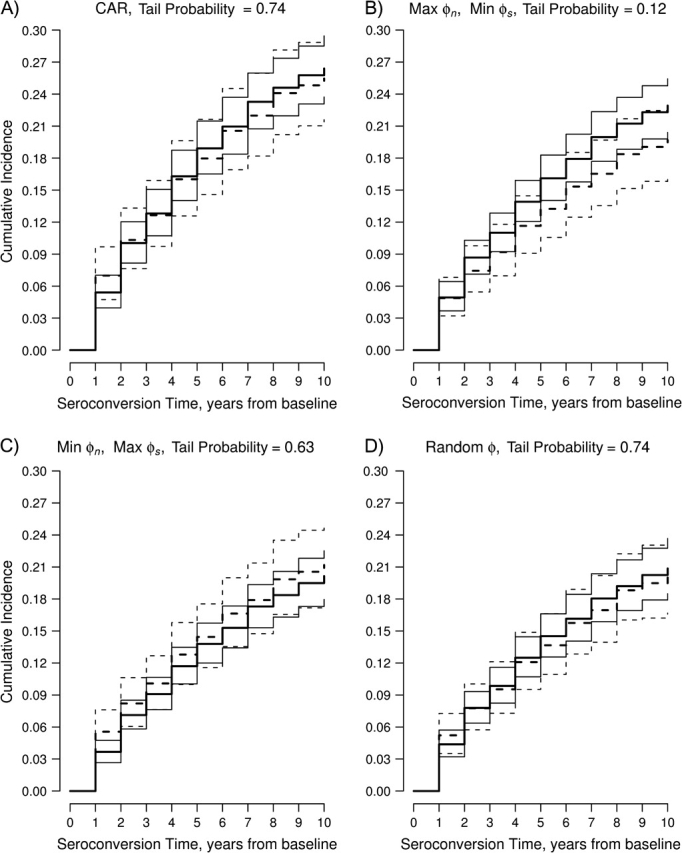
Bayesian results for the AIDS Link to Intravenous Experience (ALIVE) Study, Baltimore, Maryland, 1988–1998. Depicted across the range of elicited assumptions are the log-rank tail probabilities and the mean posterior cumulative incidences for needle-sharers (—) and nonsharers (– – –) and their 95% credible intervals (— and - - -, respectively). CAR, coarsening at random; Max, maximum; Min, minimum.

DISCUSSION

In this paper, we have described the concept of coarsening and have illustrated a framework for eliciting expert information about coarsening for sensitivity analysis. These principles, which are well-developed for missing data (3), are less developed for other types of coarsening. We have discussed how missingness mechanisms are special cases of coarsening mechanisms and, for censored data, how one can elicit and model departures from CAR.

Sensitivity analysis using expert information is preferable to ad hoc single imputation (e.g., extreme scores for missing data, interval endpoints for censoring) because the latter produces underestimated standard errors (32) and is often scientifically implausible. We also recommend performing sensitivity analyses of prior distributions on results. In ALIVE, we performed a Bayesian analysis that weighted prior assumptions of HIV incidence to be 10% of final results. The frequentist analysis weighted prior assumptions to be 0% of final results. In general, larger prior weights lead to results that are closer to the prior HIV incidence function.

ALIVE exemplifies the advantages of sensitivity analysis. Singly imputing the latest time is equivalent to $\mathbf{\text{ϕ}}=\text{∞}$. This can be seen by plugging equation 6 into equation 4 and taking the limit as ϕ_gc → ∞ for each censoring class and needle-sharing group. However, the maximum elicited ϕ_gc was log(3.0); thus, $\mathbf{\text{ϕ}}=\text{∞}$ is thought to be scientifically implausible by experts. Also note that

where ϕ = ∞ imputes interval midpoints. Compared with single imputation for interval-censored observations followed by Kaplan-Meier estimation (33), our approach allows CNAR assumptions for dropouts and uses appropriate censoring sets for deaths. In ALIVE, CAR-based analyses suggested no association between baseline needle-sharing and HIV seroconversion. These conclusions are robust to elicited assumptions about coarsening, and results make scientific sense because of the dynamic nature and potential reporting bias of needle-sharing.

Drawbacks to the proposed approach include difficulty specifying q_g(t), the subjective, potentially challenging nature of elicitation, and the need for statistical methods beyond those available in most off-the-shelf statistical packages. Additionally, while we found conclusively no evidence of a relation between baseline self-reported needle-sharing and HIV seroconversion, some sensitivity analyses may be inconclusive. For example, making the assumption of ϕ_nc = 0 and ϕ_sc = −log(1.5) for c = 1, 2, 3 (values outside the elicited range) suggests higher cumulative incidence for needle-sharers than for nonsharers (P = 0.015; data not shown).

Despite drawbacks, one cannot escape subjective inestimable assumptions for coarsened data (34). We hope that performing sensitivity analysis using elicited expert information will facilitate communication between biostatisticians, epidemiologists, and substantive experts about implicit assumptions made in standard statistical methods and their plausibility in epidemiology. Our ultimate goal is improved reporting of sensitivity analysis for coarsened data.

Glossary

Abbreviations

ALIVE

AIDS Link to Intravenous Experience

CAR

coarsening at random

CI

confidence interval

CrI

credible interval

CNAR

coarsening not at random

HIV

human immunodeficiency virus

References

- 1.Hogan JW, Roy J, Korkontzelou C. Handling drop-out in longitudinal studies. Stat Med. 2004;23(9):1455–1497. doi: 10.1002/sim.1728. [DOI] [PubMed] [Google Scholar]
- 2.White IR, Carpenter J, Evans S, et al. Eliciting and using expert opinions about dropout bias in randomized controlled trials. Clin Trials. 2007;4(2):125–139. doi: 10.1177/1740774507077849. [DOI] [PubMed] [Google Scholar]
- 3.Wood AM, White IR, Thompson SG. Are missing outcome data adequately handled? A review of published randomized controlled trials in major medical journals. Clin Trials. 2004;1(4):368–376. doi: 10.1191/1740774504cn032oa. [DOI] [PubMed] [Google Scholar]
- 4.Rubin DB. Inference and missing data. Biometrika. 1976;63(3):581–592. [Google Scholar]
- 5.Heitjan DF, Rubin DB. Ignorability and coarse data. Ann Stat. 1991;19(4):2244–2253. [Google Scholar]
- 6.Heitjan DF. Ignorability and coarse data: some biomedical examples. Biometrics. 1993;49(4):1099–1109. [PubMed] [Google Scholar]
- 7.Vlahov D, Anthony JC, Munoz A, et al. The ALIVE Study, a longitudinal study of HIV-1 infection in intravenous drug users: description of methods and characteristics of participants. NIDA Res Monogr. 1991;109:75–100. [PubMed] [Google Scholar]
- 8.Strathdee SA, Galai N, Safaiean M, et al. Sex differences in risk factors for HIV seroconversion among injection drug users: a 10-year perspective. Arch Intern Med. 2001;161(10):1281–1288. doi: 10.1001/archinte.161.10.1281. [DOI] [PubMed] [Google Scholar]
- 9.Nelson KE, Galai N, Safaeian M, et al. Temporal trends in the incidence of human immunodeficiency virus infection and risk behavior among injection drug users in Baltimore, Maryland, 1988–1998. Am J Epidemiol. 2002;156(7):641–653. doi: 10.1093/aje/kwf086. [DOI] [PubMed] [Google Scholar]
- 10.Chou R, Huffman LH, Fu R, et al. Screening for HIV: a review of the evidence for the U.S. Preventive Services Task Force. Ann Intern Med. 2005;143(1):55–73. doi: 10.7326/0003-4819-143-1-200507050-00010. [DOI] [PubMed] [Google Scholar]
- 11.Schick A, Yu Q. Consistency of the GMLE with mixed case interval-censored data. Scand J Stat. 2000;27(1):45–55. [Google Scholar]
- 12.Shardell M, Scharfstein DO, Bozzette SA. Survival curve estimation for informatively coarsened discrete event-time data. Stat Med. 2007;26(10):2184–2202. doi: 10.1002/sim.2697. [DOI] [PubMed] [Google Scholar]
- 13.Shardell M, Scharfstein DO, Vlahov D, et al. Inference for cumulative incidence functions with informatively coarsened discrete event-time data. Stat Med. 2008 doi: 10.1002/sim.3397. Sep 1 [Epub ahead of print] [DOI] [PMC free article] [PubMed] [Google Scholar]
- 14.Kalbfleisch JD, Prentice RL. The Statistical Analysis of Failure Time Data. New York, NY: John Wiley and Sons, Inc; 2002. [Google Scholar]
- 15.Satagopan JM, Ben-Porat L, Berwick M, et al. A note on competing risks in survival data analysis. Br J Cancer. 2004;91(7):1229–1235. doi: 10.1038/sj.bjc.6602102. [DOI] [PMC free article] [PubMed] [Google Scholar]
- 16.Kim HT. Cumulative incidence in competing risks data and competing risks regression analysis. Clin Cancer Res. 2007;13(2):559–565. doi: 10.1158/1078-0432.CCR-06-1210. [DOI] [PubMed] [Google Scholar]
- 17.Gill RD, van der Laan NJ, Robins JM. Coarsening at random: characterizations, conjectures and counter-examples. In: Lin DY, Fleming TR, editors. State of the Art in Survival Analysis. (Springer Lecture Notes in Statistics 123) New York, NY: Springer Publishing Company; 1997. pp. 255–294. [Google Scholar]
- 18.Heckman JJ. The common structure of statistical models of truncation, sample selection, and limited dependent variables and a simple estimator for such models. Ann Econ Soc Meas. 1976;5(4):475–492. [Google Scholar]
- 19.Little RJA. Pattern-mixture models for multivariate incomplete data. J Am Stat Assoc. 1993;88(421):125–134. [Google Scholar]
- 20.Little RJA, Wang Y. Pattern-mixture models for multivariate incomplete data with covariates. Biometrics. 1996;52(1):98–111. [PubMed] [Google Scholar]
- 21.Turnbull BW. The empirical distribution function with arbitrarily grouped, censored and truncated data. J R Stat Soc Ser B. 1976;38(3):290–295. [Google Scholar]
- 22.Rotnitzky A, Robins JM, Scharfstein DO. Semiparametric regression for repeated outcomes with nonignorable nonresponse. J Am Stat Assoc. 1998;93(444):1321–1339. [Google Scholar]
- 23.Birmingham J, Rotnitzky A, Fitzmaurice GM. Pattern-mixture and selection models for analyzing longitudinal data with monotone missing patterns. J R Stat Soc Ser B. 2003;65(1):275–297. [Google Scholar]
- 24.Kadane JB, Wolfson LJ. Experiences in elicitation. Statistician. 1998;47(1):3–19. [Google Scholar]
- 25.O'Hagan A. Eliciting prior beliefs in substantial practical applications. Statistician. 1998;47(1):21–25. [Google Scholar]
- 26.Meyer MA, Booker JM. Eliciting and Analyzing Expert Judgment: A Practical Guide. Philadelphia, PA: Society for Industrial and Applied Mathematics; 1991. [Google Scholar]
- 27.Friedman SR, Jose B, Deren S, et al. Risk factors for human immunodeficiency virus seroconversion among out-of-treatment drug injectors in high and low seroprevalence cities. The National AIDS Research Consortium. Am J Epidemiol. 1995;142(8):864–874. doi: 10.1093/oxfordjournals.aje.a117726. [DOI] [PubMed] [Google Scholar]
- 28.Wiebel W, Altman N. AIDS prevention outreach to IVDUs in four US cities. Presented at the Fourth International Conference on AIDS, Stockholm, Sweden, June 12–16, 1988. [Google Scholar]
- 29.Dempster P, Laird N, Rubin D. Maximum likelihood from incomplete data via the EM algorithm. J R Stat Soc Ser B. 1977;39(1):1–22. [Google Scholar]
- 30.Geman S, Geman D. Stochastic relaxation, Gibbs distributions, and the Bayesian restoration of images. IEEE Trans Pattern Anal Mach Intell. 1984;6(6):721–741. doi: 10.1109/tpami.1984.4767596. [DOI] [PubMed] [Google Scholar]
- 31.Cowles KP, Carlin BP. Markov chain Monte Carlo convergence diagnostics: a comparative review. J Am Stat Assoc. 1996;91(434):883–904. [Google Scholar]
- 32.Rubin DB. Multiple Imputation for Nonresponse in Surveys. New York, NY: John Wiley and Sons, Inc; 1987. [Google Scholar]
- 33.Kaplan EL, Meier P. Nonparametric estimation from incomplete observations. J Am Stat Assoc. 1958;53(282):457–481. [Google Scholar]
- 34.Kadane JB. Subjective Bayesian analysis for surveys with missing data. Statistician. 1993;42(4):415–426. [Google Scholar]