Generalized linear models with unspecified reference distribution

Abstract

We propose a new class of semiparametric generalized linear models. As with existing models, these models are specified via a linear predictor and a link function for the mean of response Y as a function of predictors X. Here, however, the “baseline” distribution of Y at a given reference mean μ₀ is left unspecified and is estimated from the data. The response distribution when the mean differs from μ₀ is then generated via exponential tilting of the baseline distribution, yielding a response model that is a natural exponential family, with corresponding canonical link and variance functions. The resulting model has a level of flexibility similar to the popular proportional odds model. Maximum likelihood estimation is developed for response distributions with finite support, and the new model is studied and illustrated through simulations and example analyses from aging research.

1. INTRODUCTION

Over the past 3 decades, generalized linear models (McCullagh and Nelder, 1989) and quasi-likelihood (QL) (Wedderburn, 1974; McCullagh, 1983) have become the bread and butter of data analysis in biostatistics and other areas of applied statistics. The QL regression models generally yield consistent estimators for regression parameters under correct specification of the mean model, without requiring knowledge of the full distribution of the response variable (Crowder, 1986). When the variance is correctly specified, the QL estimating equation is fully efficient among those linear in the data (Crowder, 1987) and the model-based standard errors obtained by treating the QL equation as the true score equation are asymptotically correct. When the variance is misspecified, the empirical or “sandwich” variance estimator provides asymptotically correct standard errors (Huber, 1967; White, 1982). QL and the empirical variance estimator therefore combine to yield a powerful set of practical data analytic tools. QL has also led to advances in robust analysis procedures for longitudinal and clustered data (Liang and Zeger, 1986), missing covariate and response data (Robins and others, 1994, 1995) and covariates measured with error (e.g. Carroll and Stefanski, 1990).

Despite clear advantages in terms of robustness, models for the mean response which ignore the full distribution of that response have some obvious drawbacks, such as the inability to make inferences about the cumulative distribution of the response. They also create difficulties in more complex modeling situations such as those involving latent predictor variables or missing covariate data because marginal likelihoods over such latent or missing data are difficult to compute or are only approximate when a full likelihood is not available. For example, longitudinal or clustered data are often modeled via random-effects models (Laird and Ware, 1982); while some of these models can be fitted via extensions of QL (Breslow and Clayton, 1993), the solution is at best an approximate one (Lin and Breslow, 1996) and a full probability model for the data would presumably yield more precise inferences. In addition, posterior prediction of random effects is hampered in the absence of a full probability model. Similarly, biased or outcome-dependent sampling models (e.g. Scott and Wild, 1986) require the application of Bayes’ Theorem to—and hence a probability model for—the model of interest in order to generate a likelihood conditional on the observation being sampled; a similar formal problem arises in missing covariate models in which the response is modeled conditional on the covariate being observed.

For these reasons, in applied work in which one of us (P. J. Rathouz) has been involved, even when a model for the mean response seems plausible, if a full probability model is desired, we have often chosen to work instead with the proportional odds model (POM) (McCullagh, 1980) or the analogous ordinal probit model. For example, in our work on child conduct problems, the outcome variable is often a count of conduct symptoms. In some analyses (e.g. Lahey and others, 2007), we model the mean of this count using Poisson (log-linear) regression with overdispersion (estimated with QL), even though the response is not truly Poisson. However, in work wherein we wish to employ random effects, we base our analysis on the POM for ordinal data (e.g. Chronis and others, 2007) because we cannot justify the Poisson distributional model for symptom counts. Similarly, in aging research with outcomes such as the number of difficulties with activities of daily living, some (e.g. Clarke and George, 2005) have used Poisson regression, accounting for overdispersion, while others (e.g. Sulander and others, 2005) have used ordinal data approaches. The advantage of the POM is that it is a fully specified probability model and therefore easily combines with random effects or latent variables (Hedeker and Gibbons, 1994). It can be inconvenient to use in applied settings, however, because the interpretation of the regression coefficients as log cumulative odds ratios rather than mean contrasts is difficult for applied audiences to understand. Additionally, the analyst is often willing to interpret regression relationships directly in terms of the mean by, for example, plotting and interpreting empirical means of the response. A regression model parameterized in terms of the mean response is therefore a desirable alternative to ordinal data regression models.

Beginning with a model for the mean, this paper takes a first step toward addressing the limitations of QL by introducing a new class of semiparametric generalized linear models (SPGLMs) with a level of flexibility similar to the POM. Models in this class are characterized by a parametric function for the mean response, specified via a linear predictor and a link function, and a nonparametric baseline distribution for the response at a given reference mean μ₀. The response distribution when the mean differs from μ₀ is then generated via exponential tilting (Barndorff-Nielsen and Cox, 1989) of the baseline distribution, yielding a response model that is a natural or linear exponential family (Morris, 1982; Jørgensen, 1987).

We believe that this class of models holds promise in a variety of applications. Our hope is that it will provide a flexible alternative to QL models for the mean when a full distributional model is desired but difficult to specify and will provide a modeling framework on which to build random effects or other latent variable models, as well as new methods for missing data or biased samples. In addition, in some settings, these models will provide flexible alternatives against which to test when the analyst believes that a parametric model may in fact hold.

In Section 2, we elaborate our new model, discuss a few of its properties, and tie it to related literature. In Section 3, we restrict attention to the case where the response distribution has a finite and known support in order to develop maximum likelihood estimation. Examples of finite support outcomes from psychiatry and aging research include counts of symptoms or disability items, modeled using linear, log-linear, or logistic regression. Section 4 contains a simulation study illustrating potential benefits of our model and providing some empirical comparisons with the POM. Section 5 contains example data analyses from aging research employing our new model, and Section 6 is a discussion.

2. MODEL AND RELATED LITERATURE

2.1. A SPGLM

Let X be a p × 1 covariate vector, and let scalar response Y be randomly sampled from the conditional distribution of (Y|X), where Y has support . Interest lies in inferences about the distribution of (Y|X). Following the traditional approach to regression modeling, define the conditional mean model

(2.1)

where η = X^Tβ is the linear predictor and g(·) is a known link function. That is, g(·) is a strictly increasing function from the open interval (m, M) ⊂ into , where m = inf() and M = sup().

Now, suppose that the probability density of (Y|X) is given by

(2.2)

where f₀(·) is a baseline density on ,

depending on f₀, and θ is chosen such that . For a fixed f₀, (2.2) is a natural exponential family (Morris, 1982) with canonical parameter θ and cumulant generating function b(·). Coupling (2.2) with mean model (2.1), model (2.1)–(2.2) is a generalized linear model (McCullagh and Nelder, 1989) with linear predictor η, link function g(·), and error distribution (2.2).

The right-hand side of (2.2) is a density ratio model (Anderson, 1972) because, for θ₁ ≠ θ₂, the log ratio of the 2 corresponding densities is linear in the data, that is, log{f(y;θ1)/f(y;θ2)} ∝(θ₁ − θ₂)y. In traditional generalized linear models, f₀ is a known component of the error distribution. For example,

for the binomial model and f₀(y) = 1/(ey!), ={0,1,…}, for Poisson data. With (2.1)–(2.2), we propose to extend the traditional framework by estimating f₀ from the data as in a density ratio model while maintaining the mean model in terms of user-specified g(μ) = η. Model (2.1)–(2.2) is thus an “SPGLM” governed by finite-dimensional mean parameter β and nonparametric reference density f₀.

As with traditional generalized linear models, the mean model and the error distribution are tied together via a canonical link function g_c(μ;f₀)≡g_c(μ) = θ, ∀ μ ∈(m,M). Writing

(2.3)

we have that the solution θ to (2.3), as an implicit function of μ, is the canonical link g_c(μ;f0) = b′₋₁(μ;f₀), which depends on f₀. We show in Appendix A (Corollary 4b) of the supplementary material (available at Biostatistics online, http://www.biostatistics.oxfordjournals.org) that for a given f₀ with bounded support , g_c(μ;f₀) exists and is a one-to-one mapping from μ ∈(m,M) onto (−∞, +∞).

As stated, model (2.1)–(2.2) is not completely identifiable. In Appendix B of the supplementary material, available at Biostatistics online, we show that f₀ in (2.2) can be replaced with any other f₀^* that is a “tilted” version of f₀, that is, f₀^*(y) = f₀(y)exp(θ₀^*y)/f₀(u exp(θ₀^*u)du for some θ_0* ∈(−∞,+∞). When this substitution is made in (2.2), then θ = g_c(μ;f₀) becomes θ^* =g_c(μ;f₀^*) =θ −θ₀^* and f(y|X;β,f₀) = f(y|X;β,f₀^*). In order to render (2.1)–(2.2) identifiable, it is therefore necessary to place an additional restriction on f₀. We also show in Appendix B that for given f₀ and μ₀^* ∈(m,M), there exists a unique f₀^* that is (i) a tilted version of f₀ and (ii) has mean μ₀^*. Without loss of generality, we thus impose the identifiability constraint on f₀ that g_c(μ₀;f₀)=0 (i.e. yf₀(y)dy = μ₀), where μ₀ ∈(m,M) is an arbitrary reference mean chosen by the user; the material in Appendix B establishes that the model is invariant to the choice of μ₀. As f₀ has the interpretation as the distribution of (Y|X) when g⁻¹(X′β)= μ₀, we recommend choosing μ₀ to be the mean or median of Y in the data or some other centrally located value appropriate for the problem at hand. Doing so ensures that f₀ has a meaningful interpretation and is not an extrapolation from the data.

If is finite of cardinality K, then f₀ is a {card() −2}-dimensional parameter after incorporating constraints f₀(y) =1 and yf₀(y)=μ₀. By contrast, if Y has infinite support, then f₀ is an infinite-dimensional parameter, similar to a baseline hazard function in the Cox proportional hazards model.

REMARK 2.1

Model (2.1)–(2.2) provides an interesting alternative to the POM. Both models have p+card()−2 parameters, including a regression model for the location with p−1 slope parameters and a nonparametric model for a baseline distribution. In addition, both models share the stochastic ordering property discussed below. The 2 models are compared via simulations and data analysis examples in Sections 4–5. The similarities between them and their equivalent level of flexibility suggest that in many cases which model the analyst chooses is more likely to be a matter of analytic goals and personal preferences than a question of one model providing a substantially better fit to the data.

2.2. Properties

We mention 2 useful properties of model (2.1)–(2.2). First, it possesses a stochastic ordering property. This property states that if for given values x₁ ≠ x₂, μ(x₁;β)<μ(x₂;β), then for all y ∈ such that m < y < M,

Second, both the interpretation and the estimation of regression parameter β are robust to unknown baseline distribution f₀. Note that (2.1)–(2.2) is specified in terms of the mean function and f₀ and that b(θ) implicitly depends on f₀. So, in general, derivatives b^(r)(θ) and in particular var(Y|X;β,f₀)=b′′(θ) will depend on f₀. However, because θ is defined as a function of μ, rather than the other way around, μ is invariant to f₀. Further, as the score function for β is X(∂μ/∂η)(Y −μ)/b′′(θ), it is easily seen (Hiejima, 1997) that μ (or β) and f₀ are orthogonal parameters (Cox and Reid, 1987). The implication is that maximum likelihood estimators (MLEs) will very generally be consistent and asymptotically normal even if f₀ is misspecified or poorly estimated or if tilting model (2.2) does not hold (Crowder, 1986), although nominal standard errors will likely be incorrect. Model (2.2) can thus be seen as a working distribution for (Y|X) around its mean; if the working model is correct, mean model inferences will be enhanced, while if it is incorrect, such results will still be valid.

2.3. Related literature

The operation of multiplying a baseline density by a positive function exp{w(θ,y)} is known as exponential tilting (Barndorff-Nielsen and Cox, 1989, Section 4.3) and has been studied extensively in the context of natural exponential families (Morris, 1982) when w(θ,y) = θh(y) for some known function h(·). Exponential tilting has been used in constructing bootstrap hypothesis tests (Davison and Hinkley, 1997), in empirical likelihood methods (Owen, 2001), and in nonparametric density estimation (Efron and Tibshirani, 1996).

A connection to other work can be made by considering models wherein the regression is specified directly in terms of canonical parameter θ, that is, θ = X^Tβ. The case when X is a scalar was studied by Birch (1963; see also McCullagh and Nelder, 1989, Section 5.2.3). When X is a vector of indicators for a factor, the multigroup density ratio model (Anderson, 1972; Fokianos and others, 2001; Fokianos, 2004) arises and gives rise to methods for biased or outcome-dependent samples such as case–control studies (Qin, 1998; Gilbert, 2004). Emphasis is on comparison of the groups via contrasts in the canonical parameter θ and/or estimation of the baseline distribution f₀. In contrast to this work, our proposal is to model the mean μ, or some user-chosen transformation thereof, as a regression on X. We believe that this will render our model substantially more useful in practice as the interpretation of the regression parameter β is independent of estimated value of the baseline distribution f₀.

Finally, Hiejima (1997) recently reexamined QL estimation using tilting and mean models similar to (2.1)–(2.2); however, that author's focus is on interpreting the QL estimator when the specified variance function does not correspond to a natural exponential family distribution.

3. MAXIMUM LIKELIHOOD ESTIMATION

We now consider estimation of model (2.1)–(2.2) for the special case of a finite known support =(y₁,…,y_K)^T of cardinality K, so that baseline density f₀ is the K × 1 vector of probabilities f₀ = {f₀(y₁),…,f₀(yK)}^T. Suppose for i =1,…,n that the X_is are either iid draws from the population or fixed by design. Given each X_i, let Y_i be independently sampled from model (2.1)–(2.2), yielding a log-likelihood function l(β,f₀)= .

The p × 1 score function for β, fixing f₀, is given by

where and θ_i =g_c(μ_i;f₀). Details of computing g_c(μ_i;f₀) are in Appendix C of the supplementary material, available at Biostatistics online. Solution of S(β;f₀)=0 yields an MLE . Fisher's expected information for β is, as usual,

Note additionally that, as μ_i does not depend on f₀, we have for y ∈ , , so that estimation of β is asymptotically unaffected by estimation of f₀. Of course, as seen by the form of _ββ, estimation of f₀ is required in order to allow the use of _ββ⁻¹ to estimate var().

Turning to baseline distribution f₀, for each y∈ , the score function for f₀(y) is given by

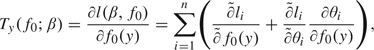where and denote the partial derivatives with respect to f₀(y) and θi, holding θi and f₀ fixed, respectively. Calculations in Appendix D of the supplementary material, available at Biostatistics online, then yield

(3.1)

Note here that Yi represents the response for the ith subject, while y represents a typical value in . Importantly, the first 2 terms in (3.1), arising from , form an unbiased estimating function for f₀(y), as does the third term. However, the third term, which is due to the fact that θ_i depends on f₀(y), asymptotically contains no information on f₀ in the sense that its derivative with respect to any f₀(y′), y′ ∈ , has expected value zero.

The K × 1 score function for f₀ for a fixed β is simply

Fairly straightforward calculations applied to the first 2 terms of Ty(f₀;β) yield Fisher's expected information as the K × K matrix _f0f0 with typical element

Note importantly that _f0β = E{−∂T(f₀;β)^T/∂β}=E{−∂S(β;f₀)/∂f₀^T}=0. So, maximum likelihood estimation of f₀ is asymptotically unaffected by estimation of β.

Solving S(β;f₀)=0 and T(f₀;β)=0 can be done simultaneously, but it is convenient to iterate between the 2, as suggested by the orthogonality between β and f₀. This is analogous to iterative estimation of regression parameters and variance–covariance parameters in fitting generalized estimating equation models (Liang and Zeger, 1986). Both equations may be solved by Fisher scoring; the algorithm for computing is well known. As for the maximum likelihood solution of T(f₀;β)=0, note that must satisfy 3 constraints: (i) 0≤f₀(y)≤1, (ii) f₀(yk)=1, and (iii) y_kf₀(y_k) =μ0. Briefly, this is accomplished by reparameterizing the model in terms of the (K−2)×1 vector h₀^*, where h₀^*(y_k)=log{f₀(y_k)}, k = 1,…,K−2. Details are provided in Appendix D.

4. SIMULATION STUDY

We conducted a simulation study of the performance of MLE (, ) in the SPGLM given by (2.1)–(2.2) using a log link function. Goals of the simulation included the following: (i) to confirm that the estimation procedure outlined in Section 3 yields consistent estimates and accurate tests and confidence intervals when the true data generation mechanism (DGM) is the SPGLM; (ii) to compare regression parameter and cumulative distribution function (cdf) estimators under a log-linear regression model with Poisson error distribution (PLLM) to those under the SPGLM when the DGM is SPGLM; and (iii) to compare the POM to the SPGLM with respect to test accuracy, power, and cdf estimation, when the DGM is either the SPGLM or the POM.

4.1. Data generation and analysis

Letting covariate vector X_i = (1,X_i1), each X_i1 was an iid draw from a standard normal distribution. Response Y_i, taking values on support ={0,1,2,3,4,5}, was generated conditionally on X_i according to 3 different DGMs. The first 2 are based on the SPGLM with link g(·)= log (·), while the third is based on the POM. In the first 2, f₀ is either a truncated Poisson or a “0-inflated” Poisson as follows. Let p₀(u) be the Poisson probability mass function with mean 1, that is, p₀(u)=1/(eu!). In the first case, we set f₀(y)=p₀(u)/. In the second, we set f₀(0)=3p₀(0)/{3p₀(0)+} and f₀(y)=p₀(y)/{3p₀(0)+}, y=1,…,5. For these 2 DGMs, we set β^T =(β₀, β₁)=(−0.7,0.2), yielding E(Y_i) ≈ 0.5 marginally over X_i.

Data for the third case were generated under the POM. Here, we set β₁ =0.3. Then, in order to ensure comparability to data generated under the SPGLM, we constructed a baseline cumulative odds function starting with the same f₀ as that given by the 0-inflated Poisson in the second DGM. Here, however, f₀ was tilted according to (2.2) for θ=g_c{exp(−0.7)}, and the resulting distribution was used for the baseline cumulative odds function. This ensured that E(Y_i|X_i=0)= exp(β₀) was the same in all 3 DGMs used in the simulations.

For each DGM, we generated 1000 replicates each with sample size n = 250. For each replicate, 3 models were fitted to the data: the PLLM, the SPGLM with log link, and the POM. Models were compared based on the values of log-likelihoods, means, and standard errors of , coverage probabilities for β, estimated cdf values, and power for detecting β₁ ≠0 using a Wald test. Additionally, in order to evaluate Type I error rates under the 3 analysis models, we generated data under the null hypothesis that β₁= 0. In all cases, Wald-based procedures were based on the estimated expected Fisher's information.

4.2. Results

Table 1 presents results for under the 2 SPGLM data–generating mechanisms. As expected, both the PLLM and the SPGLM yield approximately unbiased regression estimators, and the 2 estimators have comparable efficiency. The 95% Wald confidence interval coverage probabilities are accurate for the SPGLM, as expected, but are low for the PLLM under the 0-inflated DGM because the Poisson PLLM model does not account for the overdispersion due to the extra mass at y=0. Table 2 presents the bias and standard deviation of for the SPGLM estimators under the first 2 DGMs, demonstrating the consistency of . We conclude that the SPGLM MLEs are performing as expected.

Table 1.

Simulation results for β estimation under SPGLM data–generating mechanisms and PLLM and SPGLM models

True f0	Model	Mean		RMSE		CP
		0	1	0	1	0	1
	True β	– 0.7	0.2	—	—	—	—
Truncated Poisson	SPGLM	– 0.708	0.199	0.090	0.087	0.957	0.959
	PLLM	– 0.707	0.199	0.090	0.086	0.956	0.959
0-Inflated Poisson	SPGLM	– 0.703	0.200	0.107	0.103	0.947	0.949
	PLLM	– 0.703	0.200	0.107	0.102	0.904	0.921

RMSE: root mean square error; CP: coverage probability for 95% Wald confidence interval. True f₀ values are given in Table 2.

Table 2.

Simulation results for f₀ estimation under SPGLM data–generating mechanisms and models

Support	Truncated Poisson		0-Inflated Poisson
	True f0	Bias (SE)	True f0	Bias (SE)
0	0.367	– 0.004 (0.030)	0.471	– 0.005 (0.028)
1	0.368	0.003 (0.037)	0.232	0.003 (0.031)
2	0.185	0.002 (0.039)	0.172	0.005 (0.035)
3	0.062	0.002 (0.025)	0.085	0.001 (0.027)
4	0.016	0.002 (0.017)	0.031	– 0.002 (0.020)
5	0.003	0.001 (0.009)	0.009	– 0.002 (0.012)

SE, standard error. True β values are in Table 1.

Table 3 presents comparisons among the 3 models for the 3 DGMs. The first column presents Type I error for testing β₁=0 with a Wald test under each model, when data are generated under the null hypothesis that β^T =(−0.7,0.0). We see that both the SPGLM and the POM perform acceptably, whereas the PLLM has inflated Type I error for the 0-inflated baseline distribution. The next column presents power for detecting β₁ ≠ 0 under the alternative that β^T =(−0.7,0.2). Under the first 2 DGMs, the correctly specified SPGLM has higher power than the POM, with the power of the PLLM similar to that of the SPGLM under the truncated Poisson DGM. We ignore power results for the 0-inflated Poisson DGM under the PLLM because the Type I error rate is not correct. Under the third DGM, the correctly specified POM is more powerful. However, in each case, both the SPGLM and the POM are reasonably efficient. The log-likelihood values at the maximum give a similar picture: when either the SPGLM or the POM is the correct model, that model yields, on average, the highest likelihood value; however, the other model has comparable likelihood values and so would be a reasonable competitor in terms of overall fit of the model to the data. The last 2 columns in Table 3 present cdf parameter estimates given X =0. Again, each of the SPGLM and POM is best in terms of bias when it is correctly specified, and the PLLM is only adequate for the truncated Poisson distribution. However, the SPGLM appears to be more stable than the POM in terms of smaller standard errors in the tails of the distribution.

Table 3.

Simulation results for Type I error, power, and cdf estimation under 3 data-generating mechanisms and 3 models for estimation

Type I					(Y>1|X=0)	(Y>3|X=0)
True f0	Model	Error	Power	logL (SE)	Estimate (SE)	Estimate (SE)
Truncated	True	—	—	—	0.0892	0.0017
Poisson	SPGLM	0.056	0.62	– 229.3 (11.6)	0.0877 (0.017)	0.0017 (0.0007)
SPGLM	PLLM	0.055	0.61	– 231.0 (11.7)	0.0889 (0.013)	0.0018 (0.0006)
	POM	0.049	0.56	– 229.6 (11.6)	0.0907 (0.018)	0.0022 (0.0028)
0-Inflated	True	—	—	—	0.1258	0.0073
Poisson	SPGLM	0.047	0.47	– 235.3 (14.0)	0.1241 (0.021)	0.0073 (0.0024)
SPGLM	PLLM	0.091	0.58	– 245.9 (15.5)	0.0900 (0.016)	0.0018 (0.0007)
	POM	0.042	0.41	– 235.5 (14.1)	0.1281 (0.021)	0.0080 (0.0055)
0-Inflated	True	—	—	—	0.0892	0.0017
Poisson	SPGLM	0.047	0.62	– 227.7 (11.7)	0.0839 (0.017)	0.0016 (0.0007)
POM	PLLM	0.091	0.62	– 229.3 (11.7)	0.0876 (0.013)	0.0017 (0.0005)
	POM	0.042	0.66	– 227.4 (11.7)	0.0881 (0.018)	0.0016 (0.0025)

True β values are in Table 1. True f₀ values are given in Table 2. Type I error rates are equivalent under the 0-inflated Poisson and the POM DGMs because the true models are equivalent under the null hypothesis that β₁ = 0.

Based on these results, we expect in applications that the SPGLM and POM would both be reasonable data analysis options in the sense of having similar log-likelihood values and in terms of Type I error, power, and estimation of the conditional (on X) cdf of Y, even when the other model is the true one. The SPGLM is perhaps more stable in estimation of the tails of the cdf, and this deserves further study.

5. APPLICATION TO AGING RESEARCH: AHEAD DATA

We illustrate the use of the SPGLM given in (2.1)–(2.2) to the analysis of data from the Study of Assets and Health Dynamics Among the Oldest Old (AHEAD) (Soldo and others, 1997). AHEAD is a national longitudinal study with an initial sample of 7444 respondents aged 70 years and older and their spouses (if married). Objectives of the study include monitoring transitions in physical, functional, and cognitive health and examining the relationship of late-life changes in physical and cognitive health to patterns of dissaving and income flows. Here, we use the baseline data collected in 1993. Variable descriptions are in Table 4; complete data sample size is n = 6441.

Table 4.

Variables from baseline wave of the AHEAD study

Variable	Description
numiadl	Number of instrumental activities of daily living tasks for which the subject has some difficulty, ranging from 0 to 5.
age	Age (years) at interview of the subject.
sex	Sex of subject (1 =  female, 0 =  male).
iwr	Immediate word recall. Number of words out of 10 that subjects can list immediately after hearing them read. A measure of cognitive function.
netwc	Categorical values of net worth.

In a first analysis, we model numiadl as a function of age, sex, immediate word recall (iwr), and netwc using the SPGLM with the log link function, as well as a log-linear model with variance proportional to the mean (quasi-Poisson), and the POM. Estimates and fit statistics are given in Table 5. Comparing the SPGLM and quasi-Poisson model fits, regression estimates are as expected extremely close; the overdispersion parameter estimate of 1.48 confirms that the Poisson model is inadequate for the conditional distribution of (Y|X). The standard errors given by the quasi-Poisson and the SPGLM models are essentially equal, suggesting that, insofar as including an overdispersion parameter in the variance model corrects for effects of variance misspecification on β-inferences, the SPGLM has done an excellent job of modeling the baseline distribution.

Table 5.

Fitted log-linear and POMs for numiadl, AHEAD data. Log-linear models are estimated with SPGLM and quasi-Poisson regression

	Log-linear mean
	SPGLM			Quasi-Poisson		POM
		()	Z		()		()	Z
Intercept	– 3.61	0.337	– 10.69	– 3.62	0.337	—	—	—
age	0.05	0.004	12.74	0.05	0.004	0.07	0.005	12.71
sex:female	0.12	0.052	3.04	0.16	0.052	0.26	0.064	4.01
iwr	– 0.21	0.014	– 14.72	– 0.21	0.014	– 0.26	0.018	– 14.42
netwc:1–24k	– 0.26	0.078	– 3.28	– 0.26	0.077	– 0.45	0.113	– 4.01
netwc:25–74k	– 0.45	0.080	– 5.62	– 0.46	0.079	– 0.65	0.111	– 5.81
netwc:75–199k	– 0.69	0.081	– 8.50	– 0.69	0.081	– 0.93	0.110	– 8.46
netwc:200k–up	– 0.76	0.090	– 8.48	– 0.76	0.090	– 0.92	0.116	– 7.90
Log-likelihood	– 4951.2					– 4951.5
Scale					1.48

Turning to the SPGLM and the POM model fits, we make 2 remarks. First, based on log-likelihood values, the overall fit of the 2 models is indistinguishable. Second, while the regression parameters are not directly comparable, the corresponding Z-statistics can be compared and we see that qualitatively very similar conclusions are drawn about the effects of the predictors on numiadl. We conclude in this example that both the SPGLM and the POM are equally appropriate approaches to modeling these data, the main difference between the 2 being in the interpretation of the regression coefficients.

To further examine the ability of the SPGLM to capture the relationship of both the mean and the cdf of numiadl to iwr, we fitted a model with iwr as the sole predictor (obtaining iwr =−0.30±0.013). The fitted means (log scale) are compared to the empirical means in Figure 1. Additionally, the fitted values for Pr(iadl ≥3| iwr) compare very favorably with the empirical proportions (Figure 1, right panel); similar results were obtained for Pr(iadl≥1|iwr). The plots indicate that our model is doing well at describing both the mean and the underlying distribution function as a function of iwr. This illustrates a key advantage of the SPGLM as estimation of the conditional distribution function is not available with QL.

Fig. 1.

Fitted SPGLM model for numiadl as a function of immediate word recall (iwr), AHEAD data. Left panel: Log-mean numiadl by iwr, fitted (triangles) and observed (circles with pluses indicating 95% large-sample confidence intervals) values. Right panel: Logit of Pr(iadl ≥3) by iwr, fitted (triangles) and observed (circles with pluses indicating 95% exact binomial confidence intervals) values. Response proportions for iwr = 9 and iwr =10 were 0/105 and 0/60, so lower exact confidence limits are − ∞.

In a second analysis, we model iwr as a function of age, sex, and netwc using the SPGLM with the logistic link function g(μ)= log{μ/(10−μ)} appropriate for response Y that is the number of successes out of 10 trials. We compare this to the standard binomial model with overdispersion (quasi-binomial). In Table 6, we see that regression estimates from the 2 model fits are very close and, as in the previous example, that the standard errors from the SPGLM and the overdispersed binomial model are also very close. Additionally, because the support is the same for the binomial model and the SPGLM models, we can directly compare the log-likelihood values with a likelihood ratio test. This yields a test statistic of X² = 520 on K−2=9 df, indicating that the SPGLM fits the data significantly better than the binomial model.

Table 6.

Logistic linear models for iwr estimated with SPGLM, binomial and quasi-binomial regression, AHEAD data

	Logistic linear mean
	SPGLM			Binomial			Quasi
		()	Z	)	()	Z	()	Z
Intercept	2.22	0.134	16.54	2.22	0.120	18.50	0.134	16.58
age	– 0.04	0.002	– 23.53	– 0.04	0.001	– 26.48	0.002	– 23.74
sex:female	0.21	0.019	11.44	0.21	0.017	12.70	0.019	11.38
netwc:1–24k	0.28	0.041	6.75	0.28	0.037	7.50	0.041	6.72
netwc:25–74k	0.39	0.040	9.67	0.39	0.036	10.83	0.040	9.71
netwc:75–199k	0.55	0.039	14.16	0.55	0.034	15.89	0.038	14.24
netwc:200k–up	0.69	0.040	17.32	0.69	0.035	19.51	0.039	17.49
Log-likelihood	– 12552			– 12812
Scale							1.25

Fig. 2.

Fitted SPGLM and binomial log-logistic models for immediate word recall, AHEAD data. Left panel: Histogram of for each model. Right panel: Variance functions for the SPGLM model fit (—) and the binomial model (- - -).

To gain more insight into how the SPGLM is modeling the response distribution differently than the binomial model, we plot in Figure 2 the histograms of under the SPGLM and binomial models and the variance function (var(Y) as a function of E(Y)) generated by the fitted . It can be seen that is indeed more dispersed under the SPGLM than under the binomial model. Additionally, the variance function is clearly larger and not quadratic, thereby capturing the overdispersion in the data relative to the binomial distribution.

6. DISCUSSION

We have proposed a new class of SPGLMs for the distribution of (Y|X), characterized by a parametric function for E(Y|X) and an unspecified reference distribution to be estimated with the data. The distribution of (Y|X) for a given X is generated by an exponential tilting of the reference distribution according to a canonical parameter computed from the mean. We have shown via simulations and examples that our model yields very similar inferences for the mean parameters as commonly used overdispersed generalized linear models and enjoys a comparable level of flexibility as the popular POM, while characterizing the dependence of Y on X via the mean rather than the cumulative odds.

For count data such as the iadl or iwr responses in the AHEAD data, other semiparametric approaches are certainly available. For example, Podlich and others (2004) propose a model wherein Y_i arises as an extended Poisson process over a fixed time interval in which the rate parameter λ_i,j varies as a function of j as Y_i increments from j to j+1. Covariate effects are incorporated via a multiplicative term such as exp(X_i^Tβ), so that λ_i,j= exp(X_i^T β) λ_0,j, where λ_0,j is a nonparametric sequence of reference rates. Our model shares the same degree of flexibility as theirs by also marrying a parametric model for covariate effects with a nonparametric model for a reference distribution. It differs from theirs in that our regression is for the mean and not for a rate parameter and in that our model is not in general restricted to count data.

Straightforward generalizations of model (2.1)–(2.2) obtain through relaxing μ(·) to be a general nonlinear function of β. More involved generalizations include replacing the tilting function θy with θh(y) for known strictly monotone function h(·), estimating h(·;γ) as a function of some parameter γ, and/or using a more general tilting function w(θ,y;γ), perhaps estimated as a member of a parametric family (see, e.g. Fokianos, 2004). One use for such generalizations would be to diagnose whether the exponential tilting model (2.2) is reasonable in a given data set. These are areas for future development.

An important area for further development is the extension of these results to the case where Y has infinite support, either discrete or continuous. A major challenge in launching this work in the continuous case is to show that the nonparametric MLE of f₀ has positive mass only on the observed support. Related earlier work on this problem, for example by Vardi (1985), does not directly apply because our tilting function depends on f₀ through the parameter θ. An alternative approach is to estimate f₀ via smooth density estimation. In either case, we expect inferences about β to be robust to specification and estimation of f₀ due to the orthogonality of these 2 parameters.

FUNDING

National Cancer Institute (5PO1 CA98262) to P.J.R.

References

- Anderson JA. Separate sample logistic discrimination. Biometrika. 1972;59:19–35. [Google Scholar]
- Barndorff-Nielsen OE, Cox DR. Asymptotic Techniques for Use in Statistics. London: Chapman & Hall; 1989. [Google Scholar]
- Birch MW. Maximum likelihood in three-way contingency tables. Journal of the Royal Statistical Society Series B. 1963;25:220–233. [Google Scholar]
- Breslow NE, Clayton DG. Approximate inference in generalized linear mixed models. Journal of the American Statistical Association. 1993;88:9–25. [Google Scholar]
- Carroll RJ, Stefanski LA. Approximate quasi-likelihood estimation in models with surrogate predictors. Journal of the American Statistical Association. 1990;85:652–663. [Google Scholar]
- Chronis AM, Lahey BB, Pelham WE, Williams SH, Baumann BL, Kipp H, Jones HA, Rathouz PJ. Maternal depression and early positive parenting predict future conduct problems in young children with attention-deficit/hyperactivity disorder. Developmental Psychology. 2007;43:7–82. doi: 10.1037/0012-1649.43.1.70. [DOI] [PubMed] [Google Scholar]
- Clarke P, George LK. The role of the built environment in the disablement process. American Journal of Public Health. 2005;95:1933–1939. doi: 10.2105/AJPH.2004.054494. [DOI] [PMC free article] [PubMed] [Google Scholar]
- Cox DR, Reid N. Parameter orthogonality and approximate conditional inference. Journal of the Royal Statistical Society Series B. 1987;49:1–18. [Google Scholar]
- Crowder M. On consistency and inconsistency of estimating equations. Econometric Theory. 1986;2:305–330. [Google Scholar]
- Crowder M. On linear and quadratic estimating functions. Biometrika. 1987;74:591–597. [Google Scholar]
- Davison AC, Hinkley DV. Bootstrap Methods and Their Application. Cambridge: Cambridge University Press; 1997. [Google Scholar]
- Efron B, Tibshirani R. Using specially designed exponential families for density estimation. Annals of Statistics. 1996;24:2431–2461. [Google Scholar]
- Fokianos K. Merging information for semiparametric density estimation. Journal of the Royal Statistical Society Series B. 2004;66:941–958. [Google Scholar]
- Fokianos K, Kedem B, Qin J, Short DA. A semiparametric approach to the one-way layout. Technometrics. 2001;43:56–65. [Google Scholar]
- Gilbert PB. Goodness-of-fit tests for semiparametric biased sampling models. Journal of Statistical Planning and Inference. 2004;118:51–81. [Google Scholar]
- Hedeker D, Gibbons RD. A random-effects ordinal regression model for multilevel analysis. Biometrics. 1994;50:933–944. [PubMed] [Google Scholar]
- Hiejima Y. Interpretation of the quasi-likelihood via the tilted exponential family. Journal of the Japan Statistical Society. 1997;2:157–164. [Google Scholar]
- Huber PJ. The behavior of maximum likelihood estimates under nonstandard conditions. Proceedings of the 5th Berkeley Symposium. 1967;1:221–233. [Google Scholar]
- Jørgensen B. Exponential dispersion models. Journal of the Royal Statistical Society Series B. 1987;49:127–162. [Google Scholar]
- Lahey BB, Van Hulle CA, Waldman ID, Rodgers JL, D'onofrio BM, Pedlow S, Rathouz PJ, Keenan K. Testing descriptive hypotheses regarding sex differences in the development of conduct problems and delinquency. Journal of Abnormal Child Psychology. 2007;34:737–755. doi: 10.1007/s10802-006-9064-5. [DOI] [PubMed] [Google Scholar]
- Laird NM, Ware JH. Random effects models for longitudinal data. Biometrics. 1982;38:963–974. [PubMed] [Google Scholar]
- Liang K-Y, Zeger SL. Longitudinal data analysis using generalized linear models. Biometrika. 1986;73:13–22. [Google Scholar]
- Lin X, Breslow NE. Bias correction in generalized linear mixed models with multiple components of dispersion. Journal of the American Statistical Association. 1996;91:1007–1017. [Google Scholar]
- McCullagh P. Regression models for ordinal data (with discussion) Journal of the Royal Statistical Society Series B. 1980;42:109–142. [Google Scholar]
- McCullagh P. Quasi-likelihood functions. Annals of Statistics. 1983;11:59–67. [Google Scholar]
- McCullagh P, Nelder JA. Generalized Linear Models. 2nd edition. London: Chapman & Hall; 1989. [Google Scholar]
- Morris CN. Natural exponential families with quadratic variance functions. Annals of Statistics. 1982;10:65–80. [Google Scholar]
- Owen AB. Empirical Likelihood. Boca Raton, FL: Chapman & Hall; 2001. [Google Scholar]
- Podlich HM, Faddy MJ, Smyth GK. Semi-parametric extended Poisson process models for count data. Statistics and Computing. 2004;14:311–321. [Google Scholar]
- Qin J. Inferences for case-control and semiparametric two-sample density ratio models. Biometrika. 1998;85:619–630. [Google Scholar]
- Robins JM, Rotnitzky A, Zhao LP. Estimation of regression coefficients when some regressors are not always observed. Journal of the American Statistical Association. 1994;89:846–866. [Google Scholar]
- Robins JM, Rotnitzky A, Zhao LP. Analysis of semiparametric regression models for repeated outcomes in the presence of missing data. Journal of the American Statistical Association. 1995;90:106–121. [Google Scholar]
- Scott AJ, Wild CJ. Fitting logistic models under case-control or choice-based sampling. Journal of the Royal Statistical Society Series B. 1986;48:170–182. [Google Scholar]
- Soldo BJ, Hurd MD, Rodgers WL, Wallace RB. Asset and health dynamics of the oldest old: an overview of the AHEAD study. Journals of Gerontology, Series B, Psychological Sciences and Social Sciences. 1997;52B:1–20. doi: 10.1093/geronb/52b.special_issue.1. [DOI] [PubMed] [Google Scholar]
- Sulander T, Martelin T, Rahkonen O, Nissinen A, Uutela A. Associations of functional ability with health-related behavior and body mass index among the elderly. Archives of Gerontology and Geriatrics. 2005;40:185–199. doi: 10.1016/j.archger.2004.08.003. [DOI] [PubMed] [Google Scholar]
- Vardi Y. Empirical distributions in selection bias models. Annals of Statistics. 1985;13:178–203. [Google Scholar]
- Wedderburn RWM. Quasi-likelihood functions, generalized linear models and the Gauss-Newton method. Biometrika. 1974;61:439–447. [Google Scholar]
- White H. Maximum likelihood estimation of misspecified models. Econometrics. 1982;50:1–25. [Google Scholar]
Associated Data
This section collects any data citations, data availability statements, or supplementary materials included in this article.