

Abstract
In bioinformatics studies, supervised classification with high-dimensional input variables is frequently encountered. Examples routinely arise in genomic, epigenetic and proteomic studies. Feature selection can be employed along with classifier construction to avoid over-fitting, to generate more reliable classifier and to provide more insights into the underlying causal relationships. In this article, we provide a review of several recently developed penalized feature selection and classification techniques—which belong to the family of embedded feature selection methods—for bioinformatics studies with high-dimensional input. Classification objective functions, penalty functions and computational algorithms are discussed. Our goal is to make interested researchers aware of these feature selection and classification methods that are applicable to high-dimensional bioinformatics data.
Keywords: bioinformatics application, feature selection, penalization
INTRODUCTION
In the past decade, we have witnessed a period of unparalleled development in the field of bioinformatics [1, 2]. Among the many encountered problems, classification is one that has attracted extensive attentions. In general, classification can be defined as unsupervised or supervised, depending on if there is an observed class label. Although both are of great importance, we focus on supervised classification in this article. Supervised classification in bioinformatics is challenging partly because of the high dimensionality of the input variables. Several examples of supervised classification with high-dimensional inputs are described in ‘Examples of supervised classification in bioinformatics’ section.
When the dimension of the input variables is high compared with the number of subjects (sample size), dimension reduction or feature selection is usually needed along with classifier construction. Dimension reduction or feature selection can help to (i) provide more insights into the underlying causal relationships by focusing on a smaller number of features; (ii) generate more reliable estimates by excluding noises and (iii) provide faster and more efficient models for future studies ([3–5] and references therein).
Dimension reduction techniques, such as principal component analysis and partial least squares, construct ‘super variables’—usually linear combinations of original input variables—and use them in classification [3, 6, 7]. Although they may also lead to satisfactory classification, biomedical implications of the classifiers are usually not obvious, since all input variables are used in construction of the super variables and hence classification.
Feature selection methods can be classified into three categories, depending on their integration into the classification method [4, 5, 8]. Filter approach separates feature selection from classifier construction. Wrapper approach evaluates classification performance of selected features and keeps searching until certain accuracy criterion is satisfied. Embedded approach embeds feature selection within classifier construction.
Among feature selection methods, ‘embedded methods have the advantage that they include the interaction with the classification model, while at the same time being far less computationally intensive than wrapper methods’ [5]. In this article, we review several penalization methods, which have attracted special attentions in statistics literature in the past decade. Penalization methods belong to the family of embedded methods. They have well-defined classification objective functions, penalty terms and deterministic computational algorithms. Statistical properties of penalization methods can be easier to establish than other methods.
The goal of this article is to provide a review of several recently proposed penalized feature selection and classification methods for data with high-dimensional inputs, with special emphasis on applications of these methods in bioinformatics. This article differs from published ones in the following aspects. First, compared with review articles such as Saeys et al. [5], this article focuses only on penalization methods. We are hence able to provide a much more detailed review of such methods. Second, compared with methodological publications such as Ghosh and Chinnaiyan [9], Zhang et al. [10] and Liu et al. [11], this article does not try to propose any new methodology. Instead, it attempts to establish a unified framework which includes many published methodologies as special cases. Third, compared with statistical publications, this article focuses more on bioinformatics practice, such as real-life applications and computational aspects.
In ‘Examples of supervised classification in bioinformatics’ section, we describe a few bioinformatics examples that involve supervised classification with high-dimensional input variables. In ‘Feature selection’ section, we provide general discussions of feature selection methods and some insights into where the penalization methods fit in the big picture. Penalized feature selection and classification methods are introduced in ‘Penalized feature selection and supervised classification’section. Classification objective functions, penalty functions and computational algorithms are discussed in details. A small showcase example of cancer classification using microarray is provided in ‘Empirical performance and application’section. Several related issues are addressed in ‘Discussions’ section. Concluding remarks are given in ‘Concluding remarks’ section.
EXAMPLES OF SUPERVISED CLASSIFICATION IN BIOINFORMATICS
Genomics: cancer classification using microarray
Cancer is a genetic disease, which can be caused by mutations or defects of genes. Microarray technology makes it possible to survey the genome on a global scale. Microarray gene expression experiments have been conducted to identify biomarkers in cancers, including colon, prostate, breast, head and neck, skin, lymphoma and many others. It has been shown that up- or down-regulations of a subset of genes are associated with cancer development. Many cancer microarray studies have categorical phenotypes of interest—such as cancer occurrence, stages or subtypes—which naturally leads to supervised classification. We refer to Golub et al. [12] and West et al. [13] for representative examples.
Epigenetics: cancer classification using epigenetic measurements
In addition to having genetic causes, cancer can also be considered an epigenetic disease. Regulation by genetics involves a change in the DNA sequence, whereas epigenetic regulation involves alteration in chromatin structure and methylation of promoter region. Epigenetic measurements, such as DNA methylation patterns, have been used for cancer classification. Examples include Zukiel et al. [14], Piyathilake and Johannig [15] and references therein.
Proteomics: cancer classification using mass spectrometry
Mass spectrometry is an analytical technique that measures the mass-to-charge ratio of ions. It is generally used to find the composition of a physical sample. Some cancers affect the concentration of certain molecules in the blood, which allows early diagnosis by analyzing the blood mass spectrum. Features measured with mass spectra—often summary statistics of the peaks (for example, the peak probability contrasts in Tibshirani et al. [16])—can be used to discriminate between individuals with different cancer phenotypes. Researchers have used mass spectra for the detection of prostate, ovarian, breast, bladder, pancreatic, kidney, liver and colon cancers. See Yang et al. [17] and Diamandis and van der Merwe [18] for examples.
Proteomics: protein marker identification and classification
Protein is encoded by genes, and represented by sequence of amino acids. One of the central problems in bioinformatics is the classification of protein sequences into functional and structural families based on sequence homology. It is usually easy to sequence protein, but difficult to obtain structure. An analytic solution is to use statistical techniques and classify protein sequence data into families and super-families defined by structure/function relationships [19–21].
Proteomics: protein localization
Subcellular location of a protein is one of the key functional characters as proteins must be localized correctly at the subcellular level to have normal biological functions. Automated imaging of subcellular locations and structures can provide the ability to detect abnormalities and associate them with specific proteins. Prediction of protein subcellular localization is an important component of bioinformatics-based prediction of protein function and genome annotation, and it can aid identification of drug targets [22–24].
Remarks
Although examples described above differ significantly in techniques and application areas, their data structures share the following similarities. First, there is a categorical phenotype of interest, which may be cancer status, protein family or super-family membership, or protein location. Second, high-dimensional input variables are available for supervised classification. The input variables can be microarray gene expressions, methylation patterns, mass spectra or protein sequences. Third, such studies usually have the number of input variables much larger than the sample sizes. Thus, there is a critical demand for dimension reduction or feature selection.
FEATURE SELECTION
We show in Figure 1 a taxonomy of feature selection and dimension reduction. A similar one has been presented as Table 1 of Saeys et al. [5].
Figure 1:

A taxonomy of feature selection and dimension reduction.
Table 1:
Published articles that use penalized classification methods for microarray data (incomplete list)
| Author | Objective function | Penalty | Numerical study |
|---|---|---|---|
| Ghosh and Chinnaiyan [9] | LDA | Lasso | Simulation; microarray data |
| Zhang et al. [10] | SVM | SCAD | Simulation; microarray data; metabolism data |
| Liu et al. [11] | Likelihood | Elastic net/bridge | Simulation; methylation data; microarray data |
| Ma and Huang [32] | ROC | Lasso | Microarray data |
| Pan et al. [50] | Likelihood | Adaptive Lasso | Simulation; microarray data |
| Roth [43] | Likelihood | Lasso | Microarray data |
| Segal et al. [45] | Likelihood | Lasso | Microarray data |
| SVM | Ridge | Microarray data | |
| Shen and Tan [28] | Likelihood | Ridge | Microarray data |
| Zhu and Hastie [27] | Likelihood | Ridge | Microarray data |
| Zou and Hastie [54] | Likelihood | Elastic net | Microarray data |
Statistical methodologies that can reduce the dimensionality of input variables can be categorized depending on the relationships between original input variables and new input variables. (i) Dimension reduction methods construct new input variables using linear combinations of all original input variables. Examples include partial least squares and principal component analysis among others. (ii) Feature selection methods, which select a subset of original input variables. (iii) Hybrid methods. Most recently, researchers propose methods that combine dimension reduction and feature selection. One example is the sparse principal component analysis [25]. The hybrid methods have not been extensively used in bioinformatics yet.
Compared with dimension reduction, feature selection techniques have the potential benefits of (i) facilitating data visualization and data understanding; (ii) reducing measurement and storage requirements and (iii) reducing training and utilization times. Those properties are especially desirable for bioinformatics where a typical study measures 103–5 features on 101–3 subjects.
Feature selection methods can be further classified as filter, wrapper or embedded. We refer to table 1 of Saeys et al. [5] and the ‘Introduction’ section for related discussions. Embedded methods integrate feature selection with classifier construction (we note that this has been deemed as a drawback by some researchers). They have less computational complexity than wrapper methods. Compared with filter methods, embedded methods can better account for correlations among input variables.
Penalization methods are a subset of embedded methods, as can be seen from Figure 1. Penalization methods can be further categorized based on the classification objective functions and penalty terms, which will be discussed in details in next section.
PENALIZED FEATURE SELECTION AND SUPERVISED CLASSIFICATION
Data
For simplicity of notations, we consider binary classification only. Extensions to multi-class classification will be discussed in ‘Classification objective function’ section. Denote Y = {0, 1} as the binary phenotype of interest. For example, subjects with Y = 1 may be referred to as diseased and Y = 0 may be referred to as healthy. Let X be the length-p input variable. Suppose there are n i.i.d. copies of (X, Y) : (x1, y1), …,(xn, yn). Without loss of generality, we only consider the case that classification of Y can be based on a linear combination of the X variables, denoted as XTβ, where XT is the transpose of X, and β is the unknown, length-p regression coefficient. Nonlinear terms and interactions can be included in X as new variables.
Penalized feature selection and classification
With penalization methods, feature selection and classifier construction are achieved simultaneously by computing  , estimate of β that minimizes a penalized objective function. Classification rule can be defined as Y = 1 if
  for a cutoff c. With properly tuned penalties, estimated β can have components exactly equal to zero. Feature selection is thus achieved, since only variables with nonzero coefficients will be used in the classifier.
Specifically, we define as
| (1) |
where D represents the dataset consisting of (x1, y1), …,(xn, yn).
In [1], m is referred to as the ‘classification objective function’. We introduce different forms of m in ‘Classification objective function’ section. The penalty pen(β) in (1) controls the complexity of the model. With the penalty functions described in ‘Penalty function’ section and properly chosen λ, some components of are exactly zero. This leads to sparse classifiers and feature selection. The tuning parameter λ > 0 balances the goodness-of-fit and complexity of the model. When λ → 0, the model has better goodness-of-fit. However, since the classifier is too complex, it may have unsatisfactory prediction and be less interpretable. When λ → ∞, the classifier has fewer input variables in it. The case of λ = ∞ corresponds to the simplest classifier where no input variable is used for classification. When λ is properly tuned using cross-validation, the classifier can have satisfactory classification/prediction performance and is interpretable.
Classification objective function
In this section, we describe five extensively used classification objective functions.
Likelihood function for parametric model
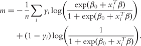
Parametric classification models assume that P(Y = 1|X) = φ(XTβ), where φ is the known link function [26]. Commonly assumed link functions include the logistic, logit, identity and probit functions. When a parametric model is assumed, m can be chosen as the negative log-likelihood function. For example, if a logistic regression model is assumed, i.e. Pr(Y = 1|X) = exp(β0 + XTβ)/(1 + exp(β0 + XTβ)), then
 |
(2) |
Parametric models for binary classification can be easily extended to multiclass cases [26]. Examples of using likelihood functions for classification in bioinformatics include Liu et al. [11], Zhu and Hastie [27], Shen and Tan [28], Shevade and Keerthi [29], and many others.
Linear discriminant function by optimal scoring
Linear discriminant analysis (LDA) has been used in microarray studies [9, 30]. Typically, LDA can be calculated using matrix algebra techniques. An effective alternative is to use the optimal scoring, where the problem of classification is re-expressed as a regression problem based on quantities known as optimal scores.
Let θ(Y) = (θ(y1), …, θ(yn))T be the n × 1 vector of quantitative scores assigned to (y1, …,yn). The optimal scoring problem involves finding the vector of coefficients β and the scoring map θ : {0, 1} → R that minimize the average squared residual:
| (3) |
The optimal scoring approach can be easily modified to incorporate multiclass cases [30].
Area under curve with receiver operating characteristics
Under the receiver operating characteristics (ROC) framework, it is assumed that P(Y = 1|X) = G(XTβ). Here G is an increasing link function. Its functional form does not need to be assumed. We refer to Pepe [31] for more details. With the ROC, classification accuracy is evaluated using the true and false positive rates (TPR and FPR), which can be defined as TPR = P(XTβ ≥ c | Y = 1), FPR = P(XTβ ≥ c | Y = 0), for a cutoff c. The ROC curve is a 2D plot of {(FPR(c), TPR(c)) : −∞ < c < ∞}. Denote  as the index sets for subjects with Y = 1 and Y = 0, with sizes nD and nH, respectively. Let XD denote the input variables of a diseased subject and XH the input variables of a healthy subject. The overall performance of a classifier can be measured by the area under curve (AUC), with larger AUC indicating better performance.
As a function of β, the empirical AUC is  where I is the indicator function. AUCe is not continuous and hence difficult to optimize.
Ma and Huang [32] proposes AUCs, a smooth approximation of the AUCe:
| (4) |
where  , and σn is the tuning parameter satisfying σn = o(n−1/2) as n → ∞.
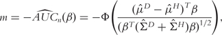
An alternative to the empirical AUC is the bi-normal AUC [31, 33]. Assume that XD and XH have normal distributions XD ∼ N(μD, ΣD) and XH ∼ N(μH, ΣH), respectively. Then the AUC can be computed as
where Φ is the normal distribution function. For a sample with n subjects, the (negative) bi-normal AUC can be estimated by
 |
(5) |
where  and
and  denote the sample mean and variance–covariance matrix, respectively.
Classification using the ROC can also be extended to multiclass problems. We refer to Mossman [34] for the volume under surface (VUS) and Provost and Domingos [35] for the one-versus-rest approaches, respectively.
Support vector machine
Under the support vector machine (SVM) framework, the binary outcome variable is recoded as  , i.e.
  . SVM is a large margin classifier which separates two classes by maximizing the margin between them. The SVM can be formulated as a penalized optimization problem with an L2 penalty
| (6) |
where β0 is the intercept term, β is the directional vector, a+ = | a |I(a > 0), 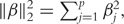 , and τ is a tuning parameter.
Usually with SVM, nonlinear kernels are needed. We refer to Cristianini and Shawe-Taylor [36] for detailed discussions. However, Zhang et al. [10] suggests that ‘when p>>n, under mild assumptions for data distribution … linear classifiers then become natural choices to discriminate two simplices’. In addition, with nonlinear kernels, once the kernels are defined, they can be treated as new input variables, and the above linear formulation is applicable. We thus provide formulation with linear kernels only.
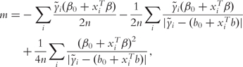
When using with other penalties, such as L1 or SCAD, the SVM objective function in [6] can be simplified by setting τ = 0. With convex penalties such as the L1 and L2, there exist efficient computational algorithms to minimize the penalized SVM function. To utilize the SVM loss function with penalties such as the SCAD, which is not convex, Zhang et al. [10] and references therein propose to approximate SVM(β) with τ = 0 by
 |
(7) |
where (b0, b) is an initial estimate of (β0, β).
Application of SVM to cancer classification using gene-expression data and protein localization prediction can be found in Guyon et al. [37] and Hua and Sun [38]. We refer to Noble [39] for a review of SVM in bioinformatics.
Remarks
All the aforementioned classification objective functions have been extensively used for binary classification in bioinformatics.
When a model can be explicitly assumed, likelihood is the most straightforward choice. It has the following properties: (i) when the underlying model is correctly assumed, likelihood based classification is optimal; (ii) with a newly observed X, likelihood approach cannot only predict the class label, but also the corresponding probability; (iii) on a negative side, likelihood-based classification relies on strong assumptions and may suffer from model mis-specification.
The LDA approach maximizes class separability. The classification objective function [3] has a simple least squares form and is easy to compute—only simple matrix operations are involved. However, the LDA approach implicitly assumes that mean is the discriminating factor (not variance), and data is normally distributed. Such assumptions may be violated and limit the applicability of LDA.
The ROC approach uses AUCs as classification objective functions. The AUC is a direct measurement of classification accuracy [31]. Classification rule obtained by maximizing the AUC is hence optimal in terms of having the largest AUC. The empirical AUC relies on much weaker assumptions compared with likelihood and LDA approaches. However, an approximation has to be used, which demands an extra tuning. The bi-normal AUC is easy to compute. However, its validity depends on the normal distribution assumption, which may be violated.
The SVM classification objective function maximizes the geometric margin between different classes. There is no explicit distribution assumption associated with SVM. With certain penalty functions, there exist efficient computational algorithms. Otherwise, an approximation may have to be introduced. In addition, SVM has no supporting incremental learning and can be sensitive to noises and outliers, which are frequently encountered in bioinformatics [40].
There is unlikely to be an objective function that is dominantly better under all scenarios. In practice, researchers may need to try different objective functions and select the proper one based on criterions such as prediction accuracy.
Penalty function
Lasso: the L1 penalty
The Lasso penalty is proposed by Tibshirani [41] and defined as
| (8) |
i.e. the L1 norm of the regression coefficient. An important property of the L1 penalty is that it can generate exact zero estimated coefficients [42]. Therefore, it can be used for feature selection.
Applications of the Lasso penalty in bioinformatics include Ghosh and Chinnaiyan [9], Shevade and Keerthi [29], Roth [43], Wei and Pan [44], Segal et al. [45] and many others. Those studies have shown that with the Lasso penalty, a small number of representative features can be selected and satisfactory classification can be achieved.
Adaptive Lasso: the weighted L1 penalty
The Lasso is in general not variable selection consistent in the sense that the whole Lasso path may not contain the true model [46]. Selection consistency of the Lasso requires an irrepresentable condition, which may not be satisfied in practice [47].
To improve the selection performance of the Lasso, Zou [48] proposes the adaptive Lasso method, which uses a weighted L1 penalty:
| (9) |
where bj is the weighted adjustment for each coefficient [48]. For linear models with n>>p, it has been proved that if bj is a  consistent estimate of βj, then the adaptive Lasso estimate is feature selection consistent under very general conditions. Also for linear models but p>>n, Huang et al. [49] shows that the adaptive Lasso can still be feature selection consistent if certain orthogonality conditions are satisfied. For classification problems, Pan et al. [50] and several other articles show that the adaptive Lasso has satisfactory classification/predication and feature selection properties with high-dimensional input.
Bridge: the Lγ penalty
The L1 Lasso penalty is a special case of the bridge penalty [42, 51, 52], which is defined as
| (10) |
For linear models with n>>p and γ < 1, the bridge penalty is feature selection consistent, even when the Lasso is not [53]. For linear models with high-dimensional input, i.e. n<<p and γ < 1, Huang et al. [53] shows that the bridge can still be feature selection consistent, if the features associated with the phenotype and those not associated with the phenotype are only weakly correlated. Numerically, Liu et al. [11] adopts a mixture penalty, which has a bridge term, in binary classification using microarray data.
Elastic net: a mixture penalty
Zou and Hastie [54] shows for linear models, when there exist highly correlated input variables, the Lasso tends to select only one of the correlated variables. With bioinformatics data, it is common that a few input features are highly correlated. One penalty that can effectively deal with high correlations is the elastic net penalty:
| (11) |
with 0 < γ ≤ 1 and η ≥ 1. That is, the elastic net is a mixture of bridge type penalties. Zou and Hastie [54] proposes γ = 1 and η = 1. In Liu et al. [11], it is extended to γ < 1 and η = 1. Applications of the elastic net in bioinformatics classification are considered in Liu et al. [11].
SCAD penalty
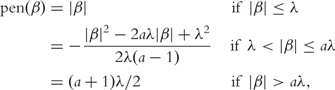
The above penalties share the same property that they increase as |βj| increases, which may cause biases in estimating large coefficients. One solution is the SCAD penalty [55]:
 |
(12) |
where a is a tuning parameter and Fan and Li [55] suggests using a = 3.7. Estimation and feature selection consistency of the SCAD penalty have been established for many distinct models with n>>p. In bioinformatics, Zhang et al. [10] and Wang et al. [56] adopt it in microarray studies and show its satisfactory performance.
Remarks
Although aforementioned penalty functions differ in their format, they all have the capability of feature selection. This can be explained by the singularity of derivatives of the penalties at zero [55].
The main advantage of Lasso is that, computationally, it is a convex optimization problem. Although it is in general not feature selection consistent, its low computational cost may compensate this drawback. In addition, multiple published articles have shown satisfactory classification performance of Lasso with high-dimensional input.
For linear models, the adaptive Lasso may fix the inconsistent feature selection problem, while still sharing the simplicity of Lasso. We expect similar properties to hold for classification models. With high-dimensional classification, selection of weights is yet to be solved. There have been published articles proposing ad hoc weights selection and showing improvement of classification using adaptive Lasso (over Lasso) with high-dimensional input. More extensive numerical studies need be conducted to draw an affirmative conclusion.
The bridge does not require any weights selection. However, there is still no satisfactory computational algorithm and an approximation may be needed (see ‘Computational algorithms’ section for more details).
The elastic net is the only penalty capable of handling ‘grouping effects’, i.e. highly correlated input variables. Such a property is especially desirable for bioinformatics studies. However, it may share the same inconsistency as the Lasso if γ = 1, or the computational difficulty as the bridge if γ < 1.
The SCAD has been very popular with statisticians in recent years because of its satisfactory theoretical properties. Zhang et al. [10] and Wang et al. [21] show its superior performance with high-dimensional classification. However, it can be computationally much harder than alternatives such as the Lasso. In addition, it involves an extra tuning parameter, which may be hard to choose objectively.
Computational algorithms
The singularity of the penalties at zero makes commonly used maximization algorithms, such as the Newton–Raphson or gradient searching, invalid. Computational algorithms for individual penalties have been proposed in early publications and summarized subsequently. A unified approach, called ‘herding lambdas’, is proposed by Friedman [57] and described.
Lasso and adaptive Lasso
The adaptive Lasso can be computed using the same algorithms as the Lasso. In early studies, the Lasso is computed with the quadratic programming (QP) or general nonlinear programming, which can be computationally intensive. For linear models, Efron et al. [58] proposes the efficient LARS approach, which is later extended to generalized linear models [59].
With high-dimensional data, an alternative approach based on boosting has been proposed by Kim and Kim [60] and later used in microarray data analysis by Ma and Huang [61]. Computational cost of the boosting approach is relatively independent of the dimensionality of input variables, which makes it especially suitable for high-dimensional data. However, the boosting approach only provides an approximation solution.
Bridge and elastic net
The elastic net penalty is the sum of the bridge and ridge penalties. The ridge penalty term is differentiable. So for the elastic net, we only need to be concerned with the bridge penalty. With γ = 1, algorithms for computing the Lasso and the augmentation algorithm in Zou and Hastie [54] are applicable for computing the elastic net estimate.
For the bridge and elastic net with γ < 1, Huang et al. [53] proposes to approximate the derivative of |βj|γ with sgn(βj)/(|βj|1−γ + ε), where sgn(βj) is the sign of βj and ε is a small positive number. In Liu et al. [11], |βj|γ is approximated with  , with a small positive ε. Then a gradient searching type algorithm can be employed.
  s smaller than a chosen cutoff are set to be zero. When ε ∼ 0, estimation with the approximated penalties is close to the exact solution.
SCAD
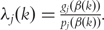
In Fan and Li [55] and Zhang et al. [10], a quadratic approximation to the SCAD penalty is proposed. The iterative successive quadratic algorithm (SQA) can then be employed. Denote βk as the estimate of β at Step k. Then pen(β) = ∑j pen(βj), where 
 . After the iteration is terminated,
  s smaller than a cutoff are set to be zero. We refer to Zhang et al. [10] for more details on this approximation.
Herding lambdas: a unified computational algorithm
We now describe a stagewise incremental approach, which can be applied to optimize objective functions with any of the above penalties, or their approximations.
Denote g(β) = −∂m(β)/∂β and its jth component as gj(β). Denote p(β) = −∂pen(β)/∂β and its jth component as pj(β). Denote ε as the fixed, small, positive increment. The ‘herding lambdas’ is an iterative approach. Denote β(k) as the estimate of β after iteration k. The algorithm can be summarized as follows:
Initialize k = 0 and β(0) = argmin{m(β) + ∞ ×pen(β)}.
If maxj |gj(β)| = 0, then stop iteration.
Compute
 .
.Denote the active set S = { j : λj(k) < 0}. If S is empty, then l = argmaxj|λj(k)|. Otherwise l = argmaxj∈S|λj(k)|.
Δ = ε|gl(β(k))|.
Update β(k) = β(k) + Δsgn(gl(β(k)))1(l), where 1(l) is the length p vector with its lth component 1 and the rest 0.
Repeat Steps 2–7 until a cross-validated criterion is satisfied.
As Friedman [57] points out that this algorithm ‘… does not always generate exactly the same path as defined by (1), it is usually close enough to maintain similar statistical properties.’ Numerical studies in Friedman [57] support this argument. The affordable computational cost and great applicability compensate the negligible loss of accuracy. Another advantage is that it can generate the complete parameter path from λ = ∞ to λ = 0, which is important when λ needs to be determined by cross-validation.
EMPIRICAL PERFORMANCE AND APPLICATION
A showcase example
Breast cancer is the second leading cause of deaths from cancer among women in the United States. Despite major progresses in breast cancer treatment, the ability to predict the metastatic behavior of tumor remains limited. The Breast Cancer study was first reported in van't Veer et al. [62]. A total of 97 lymph node-negative breast cancer patients aged 55 years old or younger participated in this study. Among them, 46 developed distant metastases within 5 years (metastatic outcome coded as 1) and 51 remained metastases free for at least 5 years (metastatic outcome coded as 0). Expression levels for 24 481 gene probes were collected using microarray. We refer to van't Veer et al. [62] for more details on experimental setup. The goal of this study is to build a statistical model that can accurately predict the risk of distant recurrence of breast cancer in a 5-year post-surgery period. The dataset is publicly available at http://www.rii.com/publications/2002/vantveer.html.
We first preprocess gene-expression data as follows: (i) Remove genes with more than 30% missing measurements. (ii) Fill in missing gene-expression measurements with median values across samples. (iii) Normalize gene expressions to have zero means and unit variances. (iv) Compute the simple correlation coefficients of gene expressions with the binary outcome. (v) Select the 500 genes with the largest absolute values of correlation coefficients.
We analyze the breast cancer data using several penalized approaches. Tuning parameters are selected using the 5-fold cross-validation. Since independent validation data is not present, we use the leave one out cross-validation (LOOCV) to evaluate the predictive power. Especially, we first remove one subject. The reduced data, with sample size n − 1, is then analyzed using penalized approaches. We note that the preprocessing and optimal tuning selection need to be conducted for each reduced data. With the statistical model generated with the reduced data, we can make prediction for the removed subject. This process is repeated over all subjects. An overall prediction error can then be computed. With different approaches, we are interested in the sets of genes identified, and LOOCV prediction error.
Logistic + Lasso. We assume the logistic regression model and use the negative log-likelihood function as the objective function. The Lasso is used for penalized gene selection. A total of 42 genes are selected. With the LOOCV, 14 subjects are misclassified.
Logistic + adaptive Lasso. Under the logistic regression model, we use the adaptive Lasso for penalized gene selection. We use the Lasso estimate as weight in the adaptive Lasso. A total of 22 genes are selected, and 14 subjects are misclassified.
Logistic + bridge. Under the logistic regression model, we use the bridge penalty with γ = 1/2 for penalized gene selection. A total of 19 genes are selected. With the LOOCV, 21 subjects cannot be properly predicted.
Logistic + elastic net. Under the logistic regression model, we also consider the elastic net penalty with γ = 1/2 and η = 2. A total of 19 genes are identified. With the LOOCV, 21 subjects cannot be properly predicted.
SVM+SCAD. We adopt the approach and software in Zhang et al. [10]. Especially, approximations are considered for both the SVM objective function and the SCAD penalty. With the 5-fold cross-validation, λ = 0.003 is selected as the optimal tuning. A total of 236 genes are selected. It is believed that the large number of identified genes is partly caused by the V-fold cross-validation. The LOOCV misclassifies 12 subjects.
Due to limited availability of software, we only consider five different combinations of objective functions and penalties, whereas there are many more possibilities. The lists of genes identified using the above five approaches are available upon request from the authors.
With different approaches, different sets of genes can be identified. Since we use the Lasso estimate as weight for the adaptive Lasso, the set of genes identified using the adaptive Lasso is a subset of those using the Lasso. For this specific dataset, the bridge and elastic net identify the same set of 19 genes, although in general this is not true. The cross-validation selects very small penalty for the SVM+SCAD. Thus a large set of genes are identified. Although the sets of identified genes can vary, all five approaches considered here have reasonably good prediction performance.
We expect performance of different approaches to be data specific. Thus, conclusions drawn from this study may not be extended to general scenarios.
General remark
The goal of this article is to provide a review of penalized methodologies that are useful in supervised bioinformatics classification studies. We provide a partial list of published articles that use penalized classification methods microarray data in Table 1. We suggest interested researchers to read those articles regarding the numerical performance of penalization methods, comparisons with alternatives, and applications. Extensive numerical studies will be needed to draw conclusions on the relative performance of penalized methods in high-dimensional classification. Such a study is of great interest, but beyond scope of this article.
DISCUSSIONS
Other forms of penalties
The ridge penalty has been used for microarray classification in Zhu and Hastie [27]. Although it is computationally simpler than the penalties discussed in ‘Penalty function’ section, it does not have a ‘built-in’ feature selection mechanism. Feature selection needs to be conducted after classifier construction. There exist other penalties that have properties similar to ridge. Although they may have satisfactory classification performance, we do not further pursue them due to their lack of feature selection capability.
Related issues
Supervised classification and feature selection with high-dimensional input are related to the following subjects: (i) prescreening, which carries out a rough screening to remove input variables unlikely to be important [63]; (ii) tuning parameter selection. The penalized approaches involve the unknown tuning parameters that should be chosen using cross-validation; (iii) classifier comparison and evaluation. Cross-validated classification accuracy, such as classification error, and number of selected features need to be compared to select the optimal classifier.
Although these issues are of great importance, they are not the focus of this article. We refer to other published papers for more detailed discussions.
Modeling of other bioinformatics data
In this article, we only consider data with categorical outcomes and classification problems. Other outcomes, such as linear or censored survival, are also commonly encountered in bioinformatics studies. Apparently, models and objective functions different from those in ‘Classification objective function’ section need to be considered. However, the general framework of penalization in section ‘Penalized feature selection and classification’ and the penalty functions in ‘Penalty function’ section are still applicable.
CONCLUDING REMARKS
Penalization methods are a family of embedded feature selection methods and have been used in bioinformatics studies with high-dimensional input. In this article, we provide a review of such methods, so that interested researchers can use them more in future bioinformatics studies. We describe five different classification objective functions and five different penalties. Corresponding computational algorithms are also discussed. A combination of any classification objective functions described in ‘Classification objective function’ section and any penalties in section ‘Penalty function’ can potentially be used for feature selection and classification. Computational and statistical aspects of several combinations, such as logistic likelihood + Lasso, logistic likelihood + elastic net, AUC + Lasso, and SVM + SCAD, have been studied in the literature cited in this article. The rest need to be studied in the future.
Acknowledgements
The authors thank the editor and three anonymous referees for their insightful comments, which have led to significant improvement of this article. The authors also thank Dr Xiaodong Lin for help with the SVM+SCAD approach. Both authors are partly supported by NIH R01CA120988-01.
Biographies
Shuangge Ma obtained his PhD in Statistics from University of Wisconsin in 2004. He was Senior Fellow in Department of Biostatistics, University of Washington from 2004 to 2006. He is Assistant Professor in Department of Epidemiology and Public Health, Yale University.
Jian Huang obtained his PhD in Statistics from University of Washington in 1994. He is Professor in Department of Statistics and Actuarial Sciences, and Department of Biostatistics, University of Iowa.
References
- Lesk AM. Introduction to Bioinformatics. USA: Oxford University Press; 2002. [Google Scholar]
- Wong S. The Practical Bioinformatician. World Scientific Publishing Company; 2004. [Google Scholar]
- Dai J, Lieu L, Rocke D. Dimension reduction for classification with gene expression microarray data. Stat Appl Genet Mol Biol. 2006;5:6. doi: 10.2202/1544-6115.1147. [DOI] [PubMed] [Google Scholar]
- Guyon I, Elisseeff A. An introduction to variable and feature selection. J Mach Learn Res. 2003;3:1157–82. [Google Scholar]
- Saeys Y, Inza I, Larranaga P. A review of feature selection techniques in bioinformatics. Bioinformatics. 2007;19:2507–17. doi: 10.1093/bioinformatics/btm344. [DOI] [PubMed] [Google Scholar]
- Boulesteix AL. Dissertation, LMU Munchen, Faculty of Mathematics, Computer Science and Statistics. 2005. Dimension reduction and classification with high dimensional microarray data. [Google Scholar]
- Nguyen DV, Rocke DM. Tumor classification by partial least squares using microarray gene expression data. Bioinformatics. 2002;18:39–50. doi: 10.1093/bioinformatics/18.1.39. [DOI] [PubMed] [Google Scholar]
- Blum A, Langley P. Selection of relevant features and examples in machine learning. Artif Intell. 1997;97:245–71. [Google Scholar]
- Ghosh D, Chinnaiyan AM. Classification and selection and biomarkers in genomic data using Lasso. J Biomed Biotechnol. 2005;2:147–54. doi: 10.1155/JBB.2005.147. [DOI] [PMC free article] [PubMed] [Google Scholar]
- Zhang H, Ahn J, Lin X, et al. Gene selection using support vector machines with non-convex penalty. Bioinformatics. 2006;22:88–95. doi: 10.1093/bioinformatics/bti736. [DOI] [PubMed] [Google Scholar]
- Liu Z, Jiang F, Tian G, et al. Sparse logistic regression with Lp penalty for biomarker identification. Stat Appl Genet Mol Biol. 2007;6:6. doi: 10.2202/1544-6115.1248. [DOI] [PubMed] [Google Scholar]
- Golub TR, Slonim DK, Tamayo P, et al. Molecular classification of cancer: class discovery and class prediction by gene expression monitoring. Science. 1999;286:531–7. doi: 10.1126/science.286.5439.531. [DOI] [PubMed] [Google Scholar]
- West M, Blanchette C, Dressmna H, et al. Predicting the clinical status of human breast cancer by using gene expression profiles. Proc Natl Acad Sci USA. 2001;98:11462–67. doi: 10.1073/pnas.201162998. [DOI] [PMC free article] [PubMed] [Google Scholar]
- Zukiel R, Nowak S, Barciszewska A, et al. A simple epigenetic method for the diagnosis and classification of brain tumors. Mol Cancer Res. 2004;2:196–202. [PubMed] [Google Scholar]
- Piyathilake C, Johannig GL. Cellular vitamins, DNA methylation and cancer risk. Am Soc Nutri Sci. 2002;132:2340S–2344S. doi: 10.1093/jn/132.8.2340S. [DOI] [PubMed] [Google Scholar]
- Tibshirani R, Hastie T, Narasimhan B, Soltys S, et al. Sample classification from protein mass spectrometry, by ‘peak probability contrasts’. Bioinformatics. 2004;20:3034–44. doi: 10.1093/bioinformatics/bth357. [DOI] [PubMed] [Google Scholar]
- Yang H, Mukomel Y, Fink E. In: Proceedings of the IEEE International Conference on Systems, Man, and Cybernetics. The Hague, The Netherlands: 2004. Diagnosis of ovarian cancer based on mass spectra of blood samples; pp. 3444–50. [Google Scholar]
- Diamandis EP, van der Merwe DE. Plasma protein profiling by mass spectrometry for cancer diagnosis: opportunities and limitations. Clin Cancer Res. 2005;11:963–5. [PubMed] [Google Scholar]
- Leslie CS, Eskin E, Cohen A, et al. Mismatch string kernels for discriminative protein classification. Bioinformatics. 2004;20:467–76. doi: 10.1093/bioinformatics/btg431. [DOI] [PubMed] [Google Scholar]
- Weston J, Leslie C, Zhou D, et al. Semi-supervised protein classification using cluster kernels. Adv Neural Inf Process Syst. 2004;16:595–602. [Google Scholar]
- Wang H, Fu Y, Sun R, et al. A SVM score for more sensitive and reliable peptide identification via tandem mass spectrometry. Pac Symp Biocomput. 2006;11:303–14. [PubMed] [Google Scholar]
- Park KJ, Kanehisa M. Prediction of protein subcellular locations by support vector machines using compositions of amino acid and amino acid pairs. Bioinformatics. 2003;19:1656–63. doi: 10.1093/bioinformatics/btg222. [DOI] [PubMed] [Google Scholar]
- Rey S, Gardy JL, Brinkman FSL. Assessing the precision of high-throughput computational and laboratory approaches for the genome-wide identification of protein subcellular localization in bacteria. BMC Genomics. 2005;6:162. doi: 10.1186/1471-2164-6-162. [DOI] [PMC free article] [PubMed] [Google Scholar]
- Yu CS, Chen YC, Lu CH, et al. Prediction of protein subcellular localization. Proteins. 2006;64:643–51. doi: 10.1002/prot.21018. [DOI] [PubMed] [Google Scholar]
- Zou H, Hastie T, Tibshirani R. Sparse principal component analysis. J Comput Graph Stat. 2006;15:265–86. [Google Scholar]
- McCullagh P, Nelder JA. Generalized Linear Models. London: Chapman and Hall; 1989. [Google Scholar]
- Zhu J, Hastie T. Classification of gene microarrays by penalized logistic regression. Biostatistics. 2004;5:427–43. doi: 10.1093/biostatistics/5.3.427. [DOI] [PubMed] [Google Scholar]
- Shen L, Tan EC. Dimension reduction based penalized logistic regression for cancer classification using microarray data. IEEE/ACM Trans Comput Biol Bioinform. 2005;2:166–75. doi: 10.1109/TCBB.2005.22. [DOI] [PubMed] [Google Scholar]
- Shevade SK, Keerthi SS. A simple and efficient algorithm for gene selecting using sparse logistic regression. Bioinformatics. 2003;19:2246–53. doi: 10.1093/bioinformatics/btg308. [DOI] [PubMed] [Google Scholar]
- Dudoit S, Fridlyand J, Speed TP, et al. Comparison of discrimination methods for the classification of tumors using gene expression data. J Am Stat Assoc. 2002;97:77–87. [Google Scholar]
- Pepe MS. The Statistical Evaluation of Medical Tests for Classification and Prediction. UK: Oxford University Press; 2003. [Google Scholar]
- Ma S, Huang J. Regularized ROC method for disease classification and biomarker selection with microarray data. Bioinformatics. 2005;21:4356–62. doi: 10.1093/bioinformatics/bti724. [DOI] [PubMed] [Google Scholar]
- Ma S, Song X, Huang J. Regularized binormal ROC method in disease classification using microarray data. BMC Bioinformatics. 2006;7:253. doi: 10.1186/1471-2105-7-253. [DOI] [PMC free article] [PubMed] [Google Scholar]
- Mossman D. Three-way ROCs. Med Decis Making. 1999;19:78–89. doi: 10.1177/0272989X9901900110. [DOI] [PubMed] [Google Scholar]
- Provost F, Domingos P. Tree induction for probability based rankings. Mach Learn. 2003;52:199–215. [Google Scholar]
- Cristianini N, Shawe-Taylor J. An Introduction to Support Vector Machines and Other Kernel-based Learning Methods. Cambridge University Press; 2000. [Google Scholar]
- Guyon I, Weston J, Barnhill S, et al. Gene selection for cancer classification using support vector machine. Mach Learn. 2004;46:389–422. [Google Scholar]
- Hua S, Sun Z. Support vector machine approach for protein subcellular localization prediction. Bioinformatics. 2001;17:721–8. doi: 10.1093/bioinformatics/17.8.721. [DOI] [PubMed] [Google Scholar]
- Noble WS. Support vector machine applications in computational biology. In: Scholkopf B, Tsuda K, Vert J, editors. Kernel Methods in Computational Biology. MIT Press; 2004. pp. 71–92. [Google Scholar]
- An J, Wang Z, Ma Z. In: Proceedings of the Second International Conference on Machine Learning and Cybernetics. Xi An, China: 2003. An incremental learning algorithm for support vector machine. [Google Scholar]
- Tibshirani R. Regression shrinkage and selection via the Lasso. JRSSB. 1996;58:267–88. [Google Scholar]
- Knight K, Fu W. Asymptotics for Lasso-type estimators. Ann Stat. 2000;28:1356–78. [Google Scholar]
- Roth V. Technical Report IAI-TR-2002-8, University of Bonn. Computer Science III; 2002. The generalized LASSO: a wrapper approach to gene selection for microarray data. http://people.inf.ethz.ch/vroth/GenLASSO/index.html. [Google Scholar]
- Wei P, Pan W. Incorporating gene functions into regression analysis of DNA-protein binding data and gene expression data to construct transcriptional networks. IEEE Trans Comput Biol Bioinform. 2006;99:1. doi: 10.1109/TCBB.2007.1062. [DOI] [PubMed] [Google Scholar]
- Segal MR, Dahlquist KD, Conklin BR. Regression approaches for microarray data analysis. J Comput Biol. 2003;10:961–80. doi: 10.1089/106652703322756177. [DOI] [PubMed] [Google Scholar]
- Leng C, Lin Y, Wahba G. A note on the LASSO and related procedures in model selection. Stat Sin. 2006;16:1273–84. [Google Scholar]
- Zhao P, Yu B. On model selection consistency of LASSO. J Mach Learn Res. 2006;7:2541–63. [Google Scholar]
- Zou H. The adaptive Lasso and its oracle properties. JASA. 2006;101:1418–29. [Google Scholar]
- Huang J, Ma S, Zhang C. Stat Sin. 2007. Adaptive Lasso for sparse high dimensional regression models. [Google Scholar]
- Pan W, Shen X, Jiang A, et al. Semi-supervised learning via penalized mixture model with application to microarray sample classification. Bioinformatics. 2006;22:2388–95. doi: 10.1093/bioinformatics/btl393. [DOI] [PubMed] [Google Scholar]
- Frank IE, Friedman JH. A statistical view of some chemometrics regression tools (with discussion) Technometrics. 1993;35:109–48. [Google Scholar]
- Fu W. Penalized regressions: the bridge versus the Lasso. J Comput Graph Stat. 1998;7:397–416. [Google Scholar]
- Huang J, Horowitz J, Ma S. Asymptotic properties of bridge estimators in sparse high-dimensional regression models. Ann Stat. 2008;36:587–613. [Google Scholar]
- Zou H, Hastie T. Regularization and variable selection via the elastic net. J Roy Stat Soc B. 2005;67:301–20. [Google Scholar]
- Fan J, Li R. Variable selection via nonconcave penalized likelihood and its oracle properties. J Am Stat Assoc. 2001;96:1348–60. [Google Scholar]
- Wang L, Chen G, Li H. Group SCAD regression analysis for microarray time course gene expression data. Bioinformatics. 2007;23:1486–94. doi: 10.1093/bioinformatics/btm125. [DOI] [PubMed] [Google Scholar]
- Friedman JH. Manuscript, Department of Statistics. Stanford University; 2006. Herding Lambdas: fast algorithms for penalized regression and classification. http://www-stat.stanford.edu/~jhf/ [Google Scholar]
- Efron B, Hastie T, Johnstone I, et al. Least angle regression (with discussion) Ann Stat. 2004;32:407–99. [Google Scholar]
- Park MY, Hastie T. L1 regularization path algorithm for generalized linear models. J Roy Stat Soc B. 2007;69:659–77. [Google Scholar]
- Kim Y, Kim J. In: Proceedings of the 21st International Conference on Machine Learning. Omnipress: Banff, Alberta, Canada; 2004. Gradient LASSO for feature selection. [Google Scholar]
- Ma S, Huang J. Additive risk survival model with microarray data. BMC Bioinformatics. 2007;8:192. doi: 10.1186/1471-2105-8-192. [DOI] [PMC free article] [PubMed] [Google Scholar]
- van't Veer LJ, Dai H, van de Vijver MJ, et al. Gene expression profiling predicts clinical outcome of breast cancer. Nature. 2002;415:530–6. doi: 10.1038/415530a. [DOI] [PubMed] [Google Scholar]
- Ma S. Empirical study of supervised gene screening. BMC Bioinformatics. 2006;7:537. doi: 10.1186/1471-2105-7-537. [DOI] [PMC free article] [PubMed] [Google Scholar]