Surface Reconstruction From Non-parallel Curve Networks

Abstract

Building surfaces from cross-section curves has wide applications including bio-medical modeling. Previous work in this area has mostly focused on connecting simple closed curves on parallel cross-sections. Here we consider the more general problem where input data may lie on non-parallel cross-sections and consist of curve networks that represent the segmentation of the underlying object by different material or tissue types (e.g., skin, muscle, bone, etc.) on each cross-section. The desired output is a surface network that models both the exterior surface and the internal partitioning of the object. We introduce an algorithm that is capable of handling curve networks of arbitrary shape and topology on cross-section planes with arbitrary orientations. Our algorithm is simple to implement and is guaranteed to produce a closed surface network that interpolates the curve network on each cross-section. Our method is demonstrated on both synthetic and bio-medical examples.

1. Introduction

Reconstructing a complete surface from incomplete data is a topic of wide interest in geometry processing. A common case of this is planar curves that represent cross-sections of a complete surface. In bio-medical modeling, for instance, contours of an anatomical structure are drawn by physicians on 2D images (such as in freehand ultrasound) or on slices of a 3D volume (such as MRI and CT scans), and a surface connecting these contours is sought which represents the structure in 3D. An example is shown in Figure 1 (a) for a human Parotid gland obtained from a CT volume.

Figure 1.

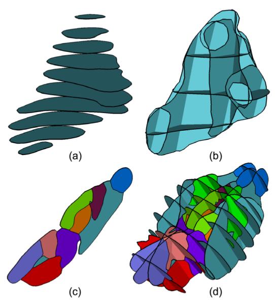
Types of cross-section curves we consider in this paper: simple closed curves on parallel (a) and non-parallel (b) planes, and curve networks (c,d).

Surface reconstruction from cross-section curves has been extensively studied for the past three decades. Previous work mostly considers connecting curves on parallel cross-sections (e.g., Figure 1 (a)), where many solutions exist (see a brief review in Section 2). Here we are interested in the more difficult problem of surface reconstruction from non-parallel cross-sections (e.g., Figure 1 (b)). The need for handling curves on non-parallel planes arises in multiple applications. In freehand 2D ultrasound, for example, both the location and orientation of each individual image plane can be freely changed through an input device that has 6 degrees of freedom. Additionally, when selecting planar slices of a 3D MRI or CT scan to specify contours, a physician often wishes to customize the orientation of each slice to better align to the imaged object. For example, the contours in Figure 1 (b) delineate the same subject as in (a) but are drawn on a set of non-parallel slices chosen by a physician to more accurately capture anatomically meaningful features.

Another demand that increasingly arises in engineering and medical applications is reconstructing objects that are segmented by different material or tissue types. This leads to curve networks that partition each cross-section plane into regions associated with multiple labels (e.g., air, muscle, bone, etc.). Figure 1 (c) shows an example curve network that represents the segmentation of the mouse brain into various anatomical structures on a single cross-section, and Figure 1 (d) shows a set of these cross-sections from which a surface representing the segmented mouse brain needs to be reconstructed. In particular, we desire the reconstruction to be a surface network that partitions the space into labelled 3D regions. Note that the simple closed curves in Figure 1 (a,b) are also a curve network where the regions labels are simply inside and outside.

1.1. Problem statement

We consider the general problem of surface reconstruction from curve networks on possibly non-parallel cross-sections. Specifically, given a set of planes partitioned by curve networks into labelled 2D regions, we desire a surface network with the following properties:

• Closed: The surface network partitions the space into labelled 3D regions, so that two regions sharing common boundary have different labels (e.g., inside and outside).

• Interpolating: The surface network interpolates the curve networks, and the labels of partitioned 3D regions are consistent with those of 2D regions on each cross-section.

To the best of our knowledge, the reconstruction problem has never been tackled at this level of generality. While a few methods were proposed for handling non-parallel cross-sections, including the very recent work of Boissonnat and Memari [BM07], these methods are restricted to simple closed curves on each cross-section. The inadequacy of such methods in handling curve networks is illustrated in Figure 2. The blue and red surfaces in (b) are formed by independently connecting the simple closed curves bounding the blue or red regions on each cross-section in (a). Note that such reconstruction inevitably leads to a result that violates the closedness criterium, as a portion of surface (pointed by the arrow in (c)) is shared by two 3D regions of a same label (red). Similar observations were made by Weinstein [Wei00] and Ju et al. [JWC*05], who proposed different methods capable of generating closed surface networks from inputs containing curve networks. However, both of these methods are restricted to parallel cross-sections.

Figure 2.

Surface reconstruction from curve networks: the input with 3 region labels: blue, red and white (a), surfaces independently constructed from simple closed curves bounding the blue or red regions (b) resulting in a non-closed partitioning of space as seen in the cut-away view (c), and a closed surface network generated by our method (d) with a cut-away view (e).

1.2. Method overview

We present a novel algorithm for surface reconstruction from non-parallel curve networks. We follow the divide-and-conquer strategy of Boissonnat and Memari [BM07] and consider the partitioning of space into cells by all cross-section planes (known as an arrangement). The core of our algorithm is the construction of a closed surface network within each partitioned cell, which generalizes the projection-based approach of [JWC*05] from between two parallel planes to within an arbitrary convex space. Unlike [BM07] or [JWC*05], our algorithm handles both parallel and non-parallel planes as well as curve networks on each plane.

The result of our algorithm, while satisfying the closedness and interpolation criteria, may exhibit a jagged appearance unsuitable for applications where smooth surfaces are desired. We next utilize existing techniques to improve the surface quality, in particular, for modelling smooth anatomical structures in bio-medical applications. We considered mesh fairing based on surface-diffusion flow [SK01, YB02,XPB06] and mesh refinement via edge-swapping and triangle splitting [PS96]. An example result is shown in Figure 2 (d,e).

Contribution

We introduce a simple and robust algorithm that is guaranteed to produce a closed surface network interpolating arbitrary curve networks on cross-sections with arbitrary (parallel or non-parallel) orientations. The method is demonstrated on both synthetic and medical examples.

2. Previous work

We start by briefly reviewing representative work on surface reconstruction from planar curves (also known as contour interpolation or contour stitching), with an emphasis on the limitation of these methods in handling complex inputs. Note that a closely related area is the interpolation or approximation of spatial curves with smooth algebraic surfaces [BI92, BIW93] or spline representations [XBE02, BCX95], where the resulting surface is either limited to simple topologies or based on an initial polyhedral surface.

2.1. Simple closed curves

Parallel cross-sections

The majority of surface reconstruction methods are developed for connecting simple closed curves lying on parallel planes. Early approaches attempted to find a polygonal tiling that connected curve loops on two neighboring planes while optimizing a quality measure [FKU77, CS78, MSS92]. Unfortunately, these tiling methods may fail to generate closed surfaces between planes containing multiple and nested curve loops. Robust handling of these more complex cases has become the focus of recent work. Among them, Boissonnat [Boi88] pioneered the method based on Dalaunay-meshing, which has been refined and improved in later work [Gei, CD99]. The methods of Herman et al. [HZB92] and Csebfalvi et al. [CNKG02] represent the 2D curves on each plane using implicit functions and extract the 3D surface by interpolating these functions. The two steps of building and interpolating the implicit functions are combined in the variational framework of Turk et al. [TO99]. Also, a number of methods [BS96,BCL96,OPC96,KSS00,BGLSS04] have been developed based on computing orthogonal projections of curves from two neighboring planes onto a common plane. For example, the method of Barequet et al. [BGLSS04] obtains intersections of projections from inside and outside regions on different planes, triangulates the intersected regions using Straight Skeletons [AA96], and lifts the triangulations in 3D to form the final surface.

Non-parallel cross-sections

Very few methods have been developed for connecting curves on non-parallel planes. Several attempts have been made [RU90, WMT*95] to extend implicit interpolation onto non-parallel planes. These methods are limited to the special case of serial planes so that the surface can be built from pieces, each of which bounded between two neighboring planes. More general approaches have been proposed by Payne and Toga [PT94], by Dance and Prager [DP], and very recently by Boissonnat and Memari [BM07], who extended the original Delaunay-meshing method from parallel cross-sections [Boi88]. A common strategy adopted in these methods is to consider a partitioning of space by all cross-section planes. Within each partitioned cell, a closed triangular mesh is extracted as the exterior of a 3D tetrahedral mesh connecting the cell boundary. In particular, Boissonnat and Memari [BM07] introduced the branching diagram to characterize the surface topology within each cell.

2.2. Curve networks

While many of the above-mentioned methods can handle curves with arbitrarily complex shape and topology, they are designed for simple closed curves that bi-partition each plane into inside and outside regions. Few attempts have been made so far to extend these approaches to handle curve networks. Weinstein [Wei00] extended implicit interpolation by representing the curve network on each plane as a multi-labelled implicit function. More recently, Ju et al. [JWC*05] extended the contour projection approach of [BGLSS04] from simple closed curves to curve networks by considering intersections of projections from regions with different labels on different planes. Note that both methods rely heavily on the fact that the curve networks reside on parallel planes, so that there is a well-defined direction (i.e., the plane normal) for implicit interpolation [Wei00] and for projection [JWC*05].

3. The algorithm

We now describe our algorithm for reconstructing a surface network from non-parallel curve networks. To handle non-parallel cross-sections, we follow the general divide-and-conquer strategy adopted in previous works [DP, BM07]. In particular, we consider the partitioning of space into cells by the set of all cross-section planes (known as the arrangement in Computational Geometry). The complete surface is built by first constructing a piece of surface within each partitioned cell, followed by stitching together pieces from neighboring cells. Note that if each surface piece is closed within the cell and interpolates the curves on the cell boundary, the result after stitching will remain closed and interpolating.

The remaining problem is how to construct a closed surface network within each cell that interpolates the curve networks on the cell boundary. To this end, we generalize the projection-based approach of [JWC*05] from a cell bounded two parallel planes to an arbitrary cell bounded by multiple intersecting planes. We will describe the basic ideas in 2D before presenting the full algorithm in 3D.

3.1. The idea in 2D

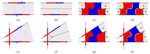
We begin by considering a simpler, lower-dimensional problem in 2D. Here the input is a set of cross-section lines, each divided by a set of points into labelled 1D regions. Two examples are shown in Figure 3 for two parallel cross-sections (a) and three non-parallel cross-sections (e). In this paper, we assume that the inputs are valid cross-sections, in that the region labelling on two intersecting cross-sections are consistent at their intersection. In this 2D setting, our goal is to reconstruct a closed curve network that interpolates the points on the cross-section lines.

Figure 3.

2D illustration of our algorithm for parallel (top) and non-parallel (bottom) cross-sections (see Section 3.1).

Following the divide-and-conquer strategy, we consider the partitioning of the plane by all the lines into cells, such as the shaded regions in Figure 3 (a,e). Note that each cell is necessarily convex. Our task is to construct a closed curve network within each cell that interpolates the points on the cell boundary.

A simple algorithm exists [JWC*05] for the case of a cell bounded by two parallel lines, like that in Figure 3 (a). The idea is to partition the cell into smaller compartments, each attached to, and labelled by, a 1D region on the cell boundary. Specifically, the cell is first divided into two compartments by the medial line between the two lines (dashed in (b)), then broken into smaller compartments by the segments that connect each point on the cell boundary to its orthogonal projection on the medial line (shown in (c)). The key observation is that the curve network separating neighboring compartments with different labels (e.g., yellow lines in (d)) is closed and interpolates the points on the cell boundary.

We extend this simple idea to cells bounded by multiple lines. The key modification we make is replacing the medial line between two parallel lines by the more general medial axes (MA) of a cell. The MA is the loci of points that are closest to two or more points on the cell boundary. Because the cell is convex, the MA consists of a set of lines or line segments (e.g., dashed lines in Figure 3 (b,f)). Note that the medial line is a special case of the MA when the cell is bounded by two parallel lines.

Using the MA, we can apply the above medial line projection algorithm to an arbitrary cell, which we will illustrate using the example in Figure 3 (e). First, the cell is partitioned into compartments by the MA (dashed in (f)) as well as the segments that connect each point on a cell boundary to its orthogonal projection on the MA (shown in (g)). Next, the curve network is extracted as the boundaries between neighboring compartments with different labels (e.g., yellow lines in (h)). As in the original algorithm [JWC*05], this curve network is closed and interpolates the points on the cell boundary.

Why medial axes

Note that the use of orthogonal projection and the MA in the algorithm is not a necessary condition for producing a closed curve network. In particular, picking other projection directions or other shapes to project onto may yield curve networks with a different topology. The advantage of using the MA and orthogonal projection is that the topology of the resulting curve networks correlates well with the sampling density of the cross-sections, and such correlation can be explicitly characterized. Formally, let A and B be two 1D regions with a common label on different boundary lines of a cell (see Figure 3 (a,e)). By the definition of the MA, A and B will both belong to the same 2D region partitioned by the resulting curve network (e.g., the blue regions in Figure 3 (d,h)) if there exists a circle inscribing the cell at a point in A and a point in B (see Figure 3 (a,e)).

3.2. The algorithm in 3D

The 2D idea can be easily extended to 3D. Our algorithm takes as its input a set of cross-section planes, each containing a curve network with partitioned 2D regions labelled. The curves are represented as piece-wise linear polylines. The algorithm first computes a partitioning of the space by all planes. Within each partitioned cell bounded by a subset of planes (like that in Figure 4 (a)), the algorithm closely follows the 2D approach to build a closed surface network interpolating the curve networks on the cell boundary:

• Step 1: Obtaining MA. Compute the MA of the cell. Since a cell is always convex, the 3D MA consists of planar pieces called sheets (dashed in Figure 4 (a)).

• Step 2: Forming compartments. The cell is partitioned into compartments by the MA sheets and polygons connecting the curve networks to their orthogonal projections on the MA. Note that new vertices may be created when projecting the curve networks onto the MA if the projections from different planes intersect with each other or with the border of a MA sheet (colored yellow in Figure4 (b)). Each compartment is attached to, and labelled by, a 2D region on the cell boundary.

• Step 3: Extracting surfaces. The surface network is extracted as the boundaries between neighboring compartments associated with different labels. Specifically, this network has two parts: triangulated portions of the MA sheets that are projected from a single region on the cell boundary (e.g., a,b,d in Figure 4 (b)) or from two regions with different labels (e.g., c in Figure 4 (b)), shown in Figure 4 (c), and triangulated polygons connecting curve network edges to their projections on the MA, shown in Figure 4 (d).

Figure 4.

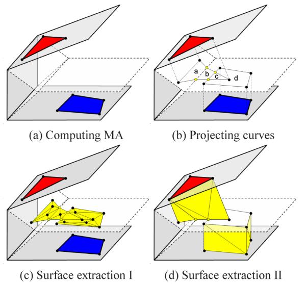
3D illustration of our algorithm within a cell.

Finally, the complete surface network is formed by stitching together surfaces constructed in neighboring cells. As in 2D, the topology of the resulting surface network correlates with the spatial configuration of the cross-sections in a well-defined manner. Specifically, two 2D regions with a same label on the cell boundary will belong to one 3D region partitioned by the surface network if there exists a sphere inscribing the cell at one point in each 2D region.

Implementation

We follow the classical tracing algorithm of Sherbrooke et al. [SPB96] to compute the MA and the Straight Skeleton method [AA96] for triangulation on the MA sheets (Figure 4 (c)). Note that, depending on the shape of the cell, the projection of curve networks on the MA may lie far away from the original data (e.g., when the dihedral angle between two planes is close to π). To prevent numerical issues, in practice we place a virtual bounding box (we used 2 times the size of the tightest bounding box of the input) around the curve networks and treat each wall of the bounding box as a new cross-section containing no curves. Note that the addition does not affect the closedness or interpolation of the result.

4. Mesh improvement

The result of our algorithm presented in the previous section, while being closed and interpolating, may exhibit a jagged and unnatural appearance. An example output is shown in Figure 5(a) for the input in Figure 2(a). Observe that all triangles are either orthogonal to the cross-section planes or aligned with the medial axes within each cell partitioned by the planes. In addition, the surface contains triangles with widely varying sizes and shapes, in part due to the sparse, non-uniform spacing between points on different cross-sections.

Figure 5.

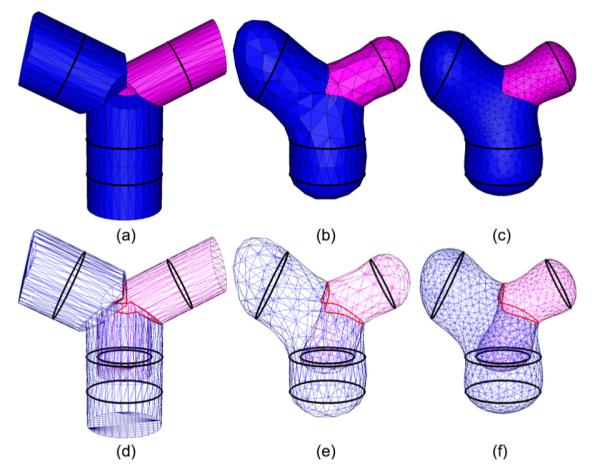
Improving the initial surface network (a) using iterative refinement and fairing at 5 (b) and 10 (c) iterations. The bottom row shows the tessellation where the non-manifold edges are highlighted.

The surface network as it is cannot be directly used in applications where smooth surfaces are desired, such as modeling anatomical structures in bio-medicine. We next resort to existing mesh fairing and refinement techniques to improve the visual appearance.

Fairing

A constraint imposed by our reconstruction goal is the interpolation of input curve networks. In particular, we demand that the resulting surface network smoothly interpolate these curves so as to exhibit a fair overall appearance. As a result, we consider a class of fairing approaches based on surface-diffusion flow [SK01, YB02, XPB06], which allows surface fairing with G¹ continuity at the constrained boundaries. Surface diffusion evolves an initial surface by moving each vertex in the surface normal direction to minimize local curvature differences. To impose the curve constraints, we follow the iterative vertex update formulation of Yoshizawa and Belyaev [YB02] while restricting vertex updates to only mesh vertices that do not lie on input curves. Additionally, to handle surface networks with a non-manifold topology, we apply Bi-Laplacian flow [KCVS98] instead of surface diffusion to the network of non-manifold vertices, where a meaningful surface normal fails to exist.

Refinement

The effect of fairing can be limited by the presence of large triangles. To this end, we adopt the multi-scale, coarse-to-fine fairing procedure similar to [KCVS98, WDSB00, Ber04]. Specifically, we adopt the refinement method of Pfeifle and Seidel [PS96], which produces a Delaunay-like triangulation via edge-swapping and triangle splitting. The refinement is controlled by a user-defined factor α that relates the density of triangles to the lengths of constraint edges. Liepa [Lie03] showed that $\alpha =\sqrt{2}$ yields a mesh that visually matches the density of the constrained vertices. Refinement and fairing are alternated in an iterative manner, with refinement performed on an increasing density factor at each iteration. Starting with α = 0, the iterations terminate when $\alpha =\sqrt{2}$. In this paper, we used 10 iterations for all models. Figure 5 shows the result of refining and fairing an initial surface network at 0, 5 and 10 iterations.

5. Examples

We test our method on both synthetic examples and bio-medical data, such as those in Figure 1, where the contours are provided by physicians and neuroscientists at the Medical School of Washington University and Pacific Northwest National Lab. The complexity of each example and the performance of our method is summarized in Table 1.

Table 1.

Performance on a 3GHz PC with 2GB memory.

Model	Region Labels	Curve Edges	Output Triangles	Surface Construction	Mesh Improvement
Parotid (parallel)	2	327	2188	47 ms	671 ms
Parotid (non-para.)	2	620	6272	203 ms	1655 ms
Horse	2	1668	16364	535 ms	4028 ms
Ring	3	282	1768	47 ms	438 ms
Brain	11	2251	23747	3588 ms	7122 ms

We begin with examples containing simple closed curves on each cross-section. Figure 6 shows the initial surface network produced by our algorithm as well as the result after mesh improvement for the Parotid gland contours in Figure1 (a,b). Another example is shown in Figure 7, where the input curves are obtained by synthetically slicing the Stanford Horse model on a selected set of planes (in this and later examples, the results are shown after mesh improvement).

Figure 6.

Reconstruction from parallel and non-parallel contours of a human Parotid gland.

Figure 7.

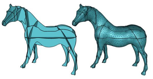
Reconstruction from synthetic slices of the Stanford Horse.

Next we present examples containing more complex curve networks. Figure 8 shows a synthetic example where a “sapphire ring” is reconstructed from curve networks on 4 planes. Note that the stone and the ring shares a common boundary outlined by non-manifold edges. Figure 9 shows the reconstruction of 3 abutting anatomical structures in the mouse brain from curve networks on 4 cross-sections. Observe that the surface network interpolates the input curve networks and partitions the space into 3D regions sharing common boundaries. Finally, Figure 10 shows the reconstruction of the whole mouse brain with 10 internal anatomical structures from 14 cross-sections.

Figure 8.

Reconstruction of a two-material sapphire ring from curve networks on four non-parallel cross-sections(a), shown as shaded surfaces (b), wireframe (c) highlighting the non-manifold edges (red), and surfaces bounding each material (d) where the ring is rotated towards the viewer to show the common boundary between the two materials.

Figure 9.

Reconstruction of 3 anatomical structures from contour curve networks on four non-parallel planes (a), shown as shaded surfaces (b), and surfaces bounding individual anatomical structures (c,d) and colored by neighboring structures.

Figure 10.

Reconstruction of 10 anatomical structures from contour curve networks on 14 non-parallel planes (a), shown as shaded surfaces (b), wireframe (c) highlighting the non-manifold edges, and surfaces bounding a subset of the structures (d)

6. Conclusion

We present a simple and robust algorithm for surface reconstruction from multi-partitioning curve networks on non-parallel cross-sections. The algorithm guarantees to produce a closed surface network that interpolates curve networks with arbitrary shape and topology on cross-sections with arbitrary orientations. In addition, the topology of the surface network correlates to the density of planes in a well-characterized manner.

The current method has a number of limitations that we wish to address in the future. First, the topology of the surface network is currently determined by on the geometric configuration of the cross-section planes, and may not reflect the true topology of the underlying object. We would like to investigate convenient means for the user to adjust this topology to their need, similar to that proposed in [JWC*05]. Second, while the initial surface generated by our algorithm is free of self-intersecting geometry, the surface after mesh improvement may lose this property. We plan to consider intersection-free alternatives for improved geometric accuracy. Third, we would like to explore domain-specific mesh improvement techniques that customize the result to particular applications. For example, in medical imaging, the grayscale 3D volume from where the contour curves are obtained, if available, would be a valuable piece of information to guide mesh fairing.

References

- [AA96].Aichholzer O, Aurenhammer F. Computing and Combinatorics. 1996. Straight skeletons for general polygonal figures in the plane; pp. 117–126. [Google Scholar]
- [BCL96].Bajaj CL, Coyle EJ, Lin K-N. Arbitrary topology shape reconstruction from planar cross sections. Graph. Models Image Process. 1996;58(6):524–543. [Google Scholar]
- [BCX95].Bajaj CL, Chen J, Xu G. Modeling with cubic a-patches. ACM Trans. Graph. 1995;14(2):103–133. [Google Scholar]
- [Ber04].Bertram M. Volume refinement fairing isosurfaces. VIS ’04: Proceedings of the conference on Visualization ’04; 2004.pp. 449–456. [Google Scholar]
- [BGLSS04].Barequet G, Goodrich MT, Levi-Steiner A, Steiner D. Straight-skeleton based contour interpolation. Graph. Models. 2004;65:323–350. [Google Scholar]
- [BI92].Bajaj CL, Ihm I. Algebraic surface design with hermite interpolation. ACM Trans. Graph. 1992;11(1):61–91. [Google Scholar]
- [BIW93].Bajaj C, Ihm I, Warren J. Higher-order interpolation and least-squares approximation using implicit algebraic surfaces. ACM Trans. Graph. 1993;12(4):327–347. [Google Scholar]
- [BM07].Boissonnat J-D, Memari P. Shape reconstruction from unorganized cross-sections. SGP ’07: Proceedings of the fifth Eurographics symposium on Geometry processing; 2007.pp. 89–98. [Google Scholar]
- [Boi88].Boissonnat J-D. Shape reconstruction from planar cross sections. Comput. Vision Graph. Image Process. 1988;44(1):1–29. [Google Scholar]
- [BS96].Barequet G, Sharir M. Piecewise-linear interpolation between polygonal slices. Computer Vision and Image Understanding. 1996;63:251–272. [Google Scholar]
- [CD99].Cheng S-W, Dey TK. Improved constructions of delaunay based contour surfaces. SMA ’99: Proceedings of the fifth ACM symposium on Solid modeling and applications; 1999; ACM Press; pp. 322–323. [Google Scholar]
- [CNKG02].Csébfalvi B, Neumann L, Kanitsar A, Gröller E. Smooth shape-based interpolation using the conjugate gradient method. Proceedings of Vision, Modeling, and Visualization; 2002.pp. 123–130. [Google Scholar]
- [CS78].Christiansen HN, Sederberg TW. Conversion of complex contour line definitions into polygonal element mosaics. Computer Graphics. 1978;13:187–192. [Google Scholar]
- [DP].Dance C, Prager R. Delaunay reconstruction from multiaxial planar cross-sections. Tech. rep.
- [FKU77].Fuchs H, Kedem ZM, Uselton SP. Optimal surface reconstruction from planar contours. Commun. ACM. 1977;20(10):693–702. [Google Scholar]
- [Gei].Geiger B. Three-dimensional modeling of human organs and its application to diagnosis and surgical planning. Tech. Rep. RR-2105.
- [HZB92].Herman GT, Zheng J, Bucholtz CA. Shape-based interpolation. IEEE Comput. Graph. Appl. 1992;12(3):69–79. [Google Scholar]
- [JWC*05].Ju T, Warren JD, Carson J, Eichele G, Thaller C, Chiu W, Bello M, Kakadiaris IA. Building 3d surface networks from 2d curve networks with application to anatomical modeling. The Visual Computer. 2005;21(8-10):764–773. [Google Scholar]
- [KCVS98].Kobbelt L, Campagna S, Vorsatz J, Seidel H-P. Interactive multi-resolution modeling on arbitrary meshes. SIGGRAPH ’98: Proceedings of the 25th annual conference on Computer graphics and interactive techniques; 1998.pp. 105–114. [Google Scholar]
- [KSS00].Klein R, Schilling A, Strasser W. Reconstruction and simplification of surfaces from contours. Graphical models. 2000;62(6):429–443. [Google Scholar]
- [Lie03].Liepa P. Filling holes in meshes. SGP ’03: Proceedings of the 2003 Eurographics/ACM SIGGRAPH symposium on Geometry processing; 2003.pp. 200–205. [Google Scholar]
- [MSS92].Meyers D, Skinner S, Sloan K. Surfaces from contours. ACM Trans. Graph. 1992;11(3):228–258. [Google Scholar]
- [OPC96].Oliva J-M, Perrin M, Coquillart S. 3d reconstruction of complex polyhedral shapes from contours using a simplified generalized voronoi diagram. Computer Graphics Forum. 1996;15(3):397–408. [Google Scholar]
- [PS96].Pfeifle R, Seidel H-P. Triangular b-splines for blending and filling of polygonal holes. GI ’96: Proceedings of the conference on Graphics interface ’96; Toronto, Ont., Canada, Canada. 1996; Canadian Information Processing Society; pp. 186–193. [Google Scholar]
- [PT94].Payne BA, Toga AW. Surface reconstruction by multiaxial triangulation. IEEE Comput. Graph. Appl. 1994;14(6):28–35. [Google Scholar]
- [RU90].Raya SP, Udupa JK. Shape-based interpolation of multidimensional objects. IEEE Transactions on Medical Imaging. 1990;9(1):32–42. doi: 10.1109/42.52980. [DOI] [PubMed] [Google Scholar]
- [SK01].Schneider R, Kobbelt L. Geometric fairing of irregular meshes for free-form surface design. Computer Aided Geometric Design. 2001;18(4):359–379. [Google Scholar]
- [SPB96].Sherbrooke EC, Patrikalakis NM, Brisson E. An algorithm for the medial axis transform of 3d polyhedral solids. IEEE Transactions on Visualization and Computer Graphics. 1996;2(1):44–61. [Google Scholar]
- [TO99].Turk G, O’brien JF. Shape transformation using variational implicit functions. SIGGRAPH ’99: Proceedings of the 26th annual conference on Computer graphics and interactive techniques; 1999; ACM Press/Addison-Wesley Publishing Co.; pp. 335–342. [Google Scholar]
- [WDSB00].Wood Z, Desbrun M, Schroder P, Breen D. Semi-regular mesh extraction from volumes. VISUALIZATION ’00: Proceedings of the 11th IEEE Visualization 2000 Conference (VIS 2000); Washington, DC, USA. 2000; IEEE Computer Society; [Google Scholar]
- [Wei00].Weinstein D. Scanline surfacing: Building separating surfaces from planar contours. VISUALIZATION ’00: Proceedings of the 11th IEEE Visualization 2000 Conference (VIS 2000); 2000; IEEE Computer Society; [Google Scholar]
- [WMT*95].Werahera P, Miller G, Taylor G, Brubaker T, Daneshgari F, Crawford E. A 3-d reconstruction algorithm for interpolation and extrapolation of planar cross sectional data. IEEE Transactions on Medical Imaging. 1995;14(4):765–771. doi: 10.1109/42.476120. [DOI] [PubMed] [Google Scholar]
- [Wol93].Wolfram S. The Mathematica Book. Wolfram Media/Cambridge University Press; 1993. [Google Scholar]
- [XBE02].Xu G, Bajaj CL, Evans S. C1 modeling with hybrid multiple-sided a-patches. Int. J. Found. Comput. Sci. 2002;13(2):261–284. [Google Scholar]
- [XPB06].Xu G, Pan Q, Bajaj C. Discrete surface modelling using partial differential equations. Computer Aided Geometric Design. 2006;23(2):125–145. doi: 10.1016/j.cagd.2005.05.004. [DOI] [PMC free article] [PubMed] [Google Scholar]
- [YB02].Yoshizawa S, Belyaev AG. Fair triangle mesh generation with discrete elastica. GMP ’02: Proceedings of the Geometric Modeling and Processing — Theory and Applications (GMP’02); Washington, DC, USA. 2002; IEEE Computer Society; p. 119. [Google Scholar]