

Abstract
Bioelectric source analysis in the human brain from scalp electroencephalography (EEG) signals is sensitive to geometry and conductivity properties of the different head tissues. We propose a low‐resolution conductivity estimation (LRCE) method using simulated annealing optimization on high‐resolution finite element models that individually optimizes a realistically shaped four‐layer volume conductor with regard to the brain and skull compartment conductivities. As input data, the method needs T1‐ and PD‐weighted magnetic resonance images for an improved modeling of the skull and the cerebrospinal fluid compartment and evoked potential data with high signal‐to‐noise ratio (SNR). Our simulation studies showed that for EEG data with realistic SNR, the LRCE method was able to simultaneously reconstruct both the brain and the skull conductivity together with the underlying dipole source and provided an improved source analysis result. We have also demonstrated the feasibility and applicability of the new method to simultaneously estimate brain and skull conductivity and a somatosensory source from measured tactile somatosensory‐evoked potentials of a human subject. Our results show the viability of an approach that computes its own conductivity values and thus reduces the dependence on assigning values from the literature and likely produces a more robust estimate of current sources. Using the LRCE method, the individually optimized four‐compartment volume conductor model can, in a second step, be used for the analysis of clinical or cognitive data acquired from the same subject. Hum Brain Mapp, 2009. © 2008 Wiley‐Liss, Inc.
Keywords: EEG, source analysis, realistic four‐compartment head modeling, in vivo conductivity estimation, brain and skull conductivity, cerebrospinal fluid, simulated annealing, finite element method, somatosensory‐evoked potentials, T1‐ and PD‐weighted MRI
INTRODUCTION
The electroencephalographic inverse problem aims at reconstructing the underlying current distribution in the human brain using potential differences measured noninvasively from the head surface. A critical component of source reconstruction is the head volume conductor model used to reach an accurate solution of the associated forward problem, i.e., the simulation of the electroencephalogram (EEG) for a known current source in the brain. The volume conductor model contains both the geometry and the electrical conduction properties of the head tissues, and the accuracy of both parameters has direct impact on the accuracy of the source analysis [Buchner et al., 1997; Gençer and Acar, 2004; Huiskamp et al., 1999; Ramon et al., 2004; Rullmann et al., 2009; Zhang et al., 2006a, b, 2008]. The practical challenges of creating patient specific models currently prohibit this degree of customization for each routine case of clinical source analysis, thus it is essential to identify the parameters that have the largest impact on solution accuracy and to attempt to customize them to the particular case.
Magnetic resonance (MR) or computed tomography (CT) imaging provides the geometry information for the brain, the cerebrospinal fluid (CSF), the skull, and the scalp [Huiskamp et al., 1999; Ramon et al., 2004; Wolters et al., 2006; Zhang et al., 2006b, 2008]. MRI has the advantage of being a completely safe and noninvasive method for imaging the head, whereas CT provides better definition of hard tissues such as bone. However, CT is not justified for routine physiological studies in healthy human subjects. In this study, we used a combination of T1‐weighted MRI, which is well suited for the identification of soft tissues (scalp, brain) and proton‐density (PD)‐weighted MRI, enabling the segmentation of the inner skull/outer CSF surface. This approach leads to an improved modeling of the CSF compartment and of the skull thickness over standard (T1)‐weighted MRI, important for a successful application of the proposed low‐resolution conductivity estimation (LRCE) method. The volume conductor model used in this study consisted of four individually and accurately shaped compartments, the scalp, skull, CSF, and brain.
Determining the second component of the head model, the conductivities of the tissues, does not have the support of a technology as capable as MRI or CT. First attempts to measure the conductivities of biological tissues were in vitro, often using samples taken from animals [Geddes and Baker, 1967]. The conductivity of human CSF at body temperature has been measured by Baumann et al. [1997] to be 1.79 S/m (average over seven subjects, ranging in age from 4.5 months to 70 years, with a standard deviation of less than 1.4% between subjects and for frequencies between 10 and 10,000 Hz). Based on the very low standard deviation determined in this study, the conductivity of the CSF compartment will be fixed to 1.79 S/m throughout this study. EEG measurements were furthermore shown to be sensitive to a correct modeling of this highly conducting compartment, which is located between the sources in the brain and the measurement electrodes on the scalp ([Huang et al., 1990; Ramon et al., 2004; Rullmann et al., 2009; Wendel et al., 2008; Wolters et al., 2006], see also discussion and further references in [Baumann et al., 1997]). In contrast, the electric conductivities of skull and brain tissues were shown to vary much stronger across individuals and within the same individual because of variations in age, disease state, and environmental factors. Latikka et al. [2001] investigated the conductivity of living intracranial tissues from nine patients under surgery. As the skull has considerably higher resistivity than the other head tissues, and thus could be expected to play an especially big role in the electric currents in the head‐much attention has been focused on determining its conductivity. Rush and Driscoll measured impedances for a half‐skull immersed in fluid [Rush and Driscoll, 1968, 1969], and since then the brain/skull conductivity ratio (in three‐compartment head models) of 80 has been commonly used in bioelectric source analysis [Homma et al., 1995]. A similar ratio of 72 averaged over six subjects was reported recently using two different in vivo approaches [Gonçalves et al., 2003a], one method using the principles of electrical impedance tomography (EIT) and the other method based on an estimation through a combined analysis of the evoked somatosensory potentials/fields (SEP/SEF). However, those results remain controversial because other studies have reported the following ratios: 15 (based on in vitro and in vivo measurements) [Oostendorp et al., 2000], 18.7 ± 2.1 (based on in vivo experiments using intracranial electrical stimulation in two epilepsy patients) [Zhang et al., 2006a], 23 (averaged value over nine subjects estimated from combined SEP/SEF data) [Baysal and Haueisen, 2004], 25 ± 7 (estimated from intra‐ and extra‐ cranial potential measurements) [Lai et al., 2005], and 42 (averaged over six subjects using EIT measurements) [Gonçalves et al., 2003b]. At this point, there is little hope of a resolution of these large discrepancies, some of which may originate in interpatient differences or natural variations over time (see, e.g., [Haueisen, 1996; Goncalves et al., 2003b]), some might result from ignoring the high conductivity of the CSF because most of the earlier studies used three‐compartment (scalp, skull, brain) head models or from ignoring the influence of realistic geometrical shape when using spherical head models, so that we propose a four‐compartment realistically shaped head modeling approach that seeks to resolve variation for each individual case by making skull and brain conductivity an additional parameter to be solved.
The growing body of evidence suggesting that the quality and fidelity of the volume conductor model of the head play a key role in solution accuracy [Cuffin, 1996; Huiskamp et al., 1999; Ramon et al., 2004; Rullmann et al., 2009] also drives the choice of numerical methods. There is a wide range of approaches including multilayer sphere models [de Munck and Peters, 1993], the boundary element method (BEM) [de Munck, 1992; Fuchs et al., 1998; Hämäläinen and Sarvas, 1989; Huiskamp et al., 1999; Kybic et al., 2005; Sarvas, 1987], the finite difference method (FDM) [Hallez et al., 2005], and the finite element method (FEM) [Bertrand et al., 1991; Haueisen, 1996; Marin et al., 1998; Ramon et al., 2004; Weinstein et al., 2000; Wolters et al., 2006; Zhang et al., 2006a, b, 2008]. The FEM offers the most flexibility in assigning both accurate geometry and detailed conductivity attributes to the model at the cost of both creating and computing on the resulting geometric model. The use of recently developed FEM transfer matrix (or lead field bases) approaches [Gençer and Acar, 2004; Weinstein et al., 2000; Wolters et al., 2004] and advances in efficient FEM solver techniques for source analysis [Wolters et al., 2004] drastically reduce the complexity of the computations so that the main disadvantage of FEM modeling no longer exists. Lanfer [2007] compared run‐time and numerical accuracy of a FEM source analysis approach (the FEM is based on a Galerkin approach applied to the weak formulation of the differential equation) using the Venant dipole model [Buchner et al., 1997] and the fast FE transfer matrix approach [Wolters et al., 2004] with a BE approach of [Zanow, 1997] (a double layer vertex collocation BE method [de Munck, 1992] using the isolated skull approach [Hämäläinen and Sarvas, 1989] and linear basis functions with analytically integrated elements [de Munck, 1992]) in combination with BE transfer matrices in an isotropic three‐layer sphere model. The reported numerical errors of the FE approach for realistic eccentricities in an isotropic three‐compartment sphere model were in the same range than those of the BEM approach, while, at the same time, the FE forward computation was faster than the BE forward computation. Additionally, similar errors and run‐times were achieved with the FE approach in anisotropic four‐compartment sphere models, showing the large flexibility of this approach.
In this article, we propose a LRCE method using simulated annealing (SA) optimization in a realistically shaped four compartment (scalp, skull, CSF, and brain) FE volume conductor model that individually optimizes the brain and the skull conductivity parameters while keeping the CSF conductivity fixed to the measurement of Baumann et al. [1997] and the scalp conductivity to the value that is commonly used in source analysis [Buchner et al., 1997; Fuchs et al., 1998; Huiskamp et al., 1999; Waberski et al., 1998; Zanow, 1997]. The LRCE method uses a geometric model, in this case based on T1‐/PD‐MRI, and evoked potential data with high signal‐to‐noise ratio (SNR) as input. The method then determines the best combination of sources within a predefined source space together with the two individually optimized brain and skull conductivity values over a discrete parameter space, i.e., for each source and for each tissue conductivity, the user has to define a reasonable set of a priori values. We evaluate the accuracy of the LRCE method in simulation studies before applying it to tactile somatosensory‐evoked potentials (SEP) with the focus on establishing the best values for the individual brain and skull conductivity. Besides using our new method for an improved source analysis of, e.g., SEP or auditory‐evoked potentials (AEP) (i.e., EEG data with a rather simple underlying source structure and a well‐controlled and high SNR), the major future perspective for the LRCE is to provide an individually optimized volume conductor model (by means of exploiting the SEP/AEP data) that can then be used in a second step for the analysis of clinical or cognitive EEG data of the same subject/patient.
THEORY
Finite Element Method‐Based Forward Problem
In the considered low‐frequency band (frequencies below 1,000 Hz), the capacitive component of tissue impedance, the inductive effect, and the electromagnetic propagation effect can be neglected so that the relationship between bioelectric fields and the underlying current sources in the brain can be represented by the quasi‐static Maxwell equation
| (1) |
with homogeneous Neumann boundary conditions at the head surface
| (2) |
and a reference electrode with given potential, i.e.,  , where σ is the conductivity distribution, ϕ is the scalar electric potential,
  is the primary (impressed) current, Ω the head domain, Γ its surface, and
  the surface normal at Γ [Plonsey and Heppner, 1967; Sarvas, 1987]. The primary current is generally modeled by a mathematical dipole at position
  with the moment
  [Sarvas, 1987]. For a given primary current and conductivity distribution, the potential can be uniquely determined for what is known as the bioelectric forward problem.
For the numerical approximation of Eqs. (1) and (2) in combination with the reference electrode, we use the FE method. Different FE approaches for modeling the source singularity are known from the literature: a subtraction approach [Bertrand et al., 1991], a partial integration direct method [Weinstein et al., 2000], and a Venant direct method [Buchner et al., 1997]. In this study, we used the Venant approach based on comparison of the performance of all three in multilayer sphere models, which suggested that for sufficiently regular meshes, it yields suitable accuracy over all realistic source locations [Lanfer, 2007; Wolters et al., 2007a, b]. This approach has the additional advantage of high computational efficiency when used in combination with the FE transfer matrix approach [Wolters et al., 2004]. We used standard piecewise linear basis functions  for
for  , where
  is the i‐th FE node, and
  for all j≠i. The potential is projected into the FE space, i.e.,
  , where N is the number of FE nodes. Standard variational and FE techniques for Eqs. (1) and (2) yield the linear system
 |
where A is the stiffness matrix with dimension N × N,  the coefficient vector for ϕh(N×1),
  the Venant approach right‐hand‐side vector (N×1) [Buchner et al., 1997; Wolters et al., 2007a], and <·,·> the scalar product. A key feature of this study was to pursue solutions that achieve high computational efficiency. Let us assume that the S electrodes directly correspond to FE nodes at the surface of the head model (otherwise, interpolation is needed). It is then easy to determine a restriction matrix B∈ ℜ(S−1)×N, which has only one nonzero entry with the value 1 in each row and which maps the potential vector
  onto the potential vector
  at the (S−1) nonreference EEG electrodes,
  . With the following definition of the (S−1)×N transfer matrix for the EEG, T := BA
−1, a direct mapping of an FE right‐hand side vector
. With the following definition of the (S−1)×N transfer matrix for the EEG, T := BA
−1, a direct mapping of an FE right‐hand side vector  onto the unknown electrode potentials
  is given. It was shown in Wolters et al. [2004] how the transfer matrix T can efficiently be computed using an algebraic multigrid preconditioned conjugate gradient (AMG‐CG) method. Note that
  has only C nonzero entries (with C being the number of neighbors of the closest FE node to the source) so that
  only amounts in 2·(S−1)·C operations. Thus the resulting combination of the transfer matrix approach with the Venant method leads to implementations that are especially efficient [Lanfer, 2007], an essential feature for our study as will become clear in section “low‐resolution conductivity estimation.”
The Inverse Problem
Dipole fit in a discrete influence space
The nonuniqueness of the EEG inverse problem requires a combination of a viable forward problem, anatomical information, and a priori constraints on some aspect(s) of the solution. Here, we followed a dipole fit procedure that restricted the number of active sources to an application dependent number, K, of some few dipoles [Mosher et al., 1992; Scherg and von Cramon, 1985]. In addition, we defined an influence space with R discrete permissible source locations that was constrained to lay within the cortical gray matter. Given this influence space, the S scalp electrode locations, and a fixed volume conductor, we used the fast FE forward computation methods from section “finite element method‐based forward problem” to compute a lead field matrix, L, which mapped sources directly to electrode potentials:
where  is a current source vector of dimension 3R×1 because we do not use the normal constraint, i.e., sources at the discrete source space nodes can have orientations in any direction.
  is the simulated potential vector of dimension S×1 and L has dimension S×3R.
Because the potential depends linearly on the source moment (dipole orientation and strength) and nonlinearly on the source location, we use a two‐phase approach for source analysis [Buchner et al., 1997; Wolters et al., 1999]. We start with K initial source locations that are proposed by the nonlinear optimization procedure SA (see section “globally minimizing the cost function”) and apply a linear least squares fit to the EEG data that determines uniquely the linear source orientation and strengths parameters,  . The numerical solver for the linear least squares procedure employed a truncated singular value decomposition for the minimization [Wolters et al., 1999], based on a cost function, g
f, that is the L
2 norm of the difference between the simulated potential,
. The numerical solver for the linear least squares procedure employed a truncated singular value decomposition for the minimization [Wolters et al., 1999], based on a cost function, g
f, that is the L
2 norm of the difference between the simulated potential,  , and the measured EEG potential,
  :
:
In this equation,  indicates the reduced lead field matrix for the current choice of source locations
  with
with  the k‐th source location (1 ≤ k ≤ K).
Globally minimizing the cost function
Because the volume conduction properties are incorporated in the lead field matrix L r, the free nonlinear optimization parameters in this case are only the source locations. There is the choice between local optimization methods such as the Nelder‐Mead simplex approach [Nelder and Mead, 1965] or the Levenberg‐Marquardt algorithm [Marquardt, 1963] and global optimization approaches such as SA from combinatorial optimization [Kirkpatrick et al., 1983] or genetic algorithms [Kjellström, 1996]. In our study, we decided for SA optimization because the challenge of local optimizers lies in determining the initial estimation of multiple parameters in the presence of local minima, and the global SA optimizer, often used when the search space is discrete as in our study, is generally more effective in localizing multiple parameters because it eliminates the need for high‐quality initial estimates [Buchner et al., 1997; Gerson et al., 1994; Haneishi et al., 1994; Uutela et al., 1998; Wolters et al., 1999]. A stochastic Metropolis acceptance test prevents the SA search from getting trapped in local minima as long as the cooling schedule is slow enough [Geman and Geman, 1984; Hütten, 1993; Metropolis et al., 1953]. For the cooling schedule, a so‐called temperature t regulates the acceptance probability. Throughout the optimization process, t decreases according to a cooling rate f t. Initially, t is set to a high value, resulting in the acceptance of most new parameters (with even larger g f) and as the temperature decreases by means of f t, it is less likely for new parameters (with larger g f) to be accepted. This enables the search to focus on the vicinity of the minima at the later stages of the optimization process.
Low‐Resolution Conductivity Estimation
The proposed LRCE method adds electrical tissue conductivities as additional optimization parameters to the cost function to the already parameterized source locations. Here, the set of optimization parameters including the conductivities was
where L is the number of tissue compartments and σl is the conductivity parameter for the l‐th tissue compartment (1 ≤ l ≤ L). Each source location  was allowed to vary within the defined discrete influence space as described in section “the inverse problem.” The conductivity σl of tissue compartment l was allowed to have its value from a predefined discrete set of possible conductivity values
Here, H l is the number of possible conductivity values for tissue compartment l. We could choose H l to be a large number (high resolution) for tissue l, but this would strongly increase computational costs and might be rather unrealistic given the limited SNR in measured EEG data. Therefore, we confined it to a rather small set of conductivity values (e.g., the different measured and estimated values for the considered head tissue that can be found in the literature).
Given the influence source space and the electrode locations, we precomputed a set of lead field matrices and collected them in Λ, which corresponded to all possible combinations of conductivity values for all tissue compartments of interest. This resulted in the number  of lead field matrices in Λ.
| (3) |
with L(σ,···,σ) being the (S×3R) lead field matrix for the specific choice of conductivities. During each iteration of the SA method, the set of optimization parameters includes not just a new estimate of the bioelectric source, but a new configuration of both sources and conductivities in which we allow changing the value of only one parameter chosen randomly per iteration. By limiting the choice of conductivities to a discrete set of values, we maintain computational efficiency by applying the associated precomputed lead field matrix from the set Λ. The total number of possible configurations for sources and conductivities is
| (4) |
The SA optimizer searches for an optimal configuration of dipole source locations  and tissue conductivities σ = (σ1,···,σL) that ensure the best fit to the measured data:
The following summarizes the general procedure of the LRCE:
Define the discrete influence space with R nodes.
Fix the number K of sources to be fitted.
For all L tissue compartments, define a discrete set of conductivity values, i.e., fix all σ, 1 ≤ h l ≤ H l, 1 ≤ l ≤ L.
Precompute Λ corresponding to each of the possible conductivity combinations using the fast FE transfer matrix approach in combination with the AMG‐CG from section “finite element method‐based forward problem.”
Repeat:
– Allow SA optimizer to choose a configuration of source locations
 and conductivities σ = (σ1,···,σL).
– Get lead field matrix L r(σ) for the chosen source and conductivity configuration.
– Compute
 with respect to source moments
  .
.Until cost function value meets a tolerance criterion or the number of iterations exceeds a limit.
METHODS AND MATERIALS
Registration and Segmentation of MR Images
To carry out the LRCE analysis requires the construction of detailed realistic head models, in this case from MR image data. Here, we outline the steps for constructing such a model. Our approach emphasizes accurate modeling of the CSF and skull compartments [Cuffin, 1996; Huiskamp et al., 1999; Ramon et al., 2004; Rullmann et al., 2009; Wendel et al., 2008; Wolters et al., 2006]. The influence of the skull thickness is closely related to the influence of skull conductivity, and therefore especially important for a successful application of the presented LRCE algorithm [Cuffin, 1996; Huiskamp et al., 1999; Ramon et al., 2004]. To achieve the required accuracy of the head models, we made use of a combination of two different MRI modalities applied to a single subject. T1‐weighted MRI is well suited for the segmentation of tissue boundaries like gray matter, outer skull, and scalp. In contrast, the identification of the inner skull surface (defining thicknesses of skull and CSF compartment) is more successful from a proton density MRI (PD‐MRI) sequence because the difference in the quantity of water protons between intracranial and bone tissues is large. T1‐ and PD‐MR imaging of a healthy 32‐year‐old male subject was performed, the images were aligned and segmented in a realistic four compartment (scalp, skull, CSF, brain) volume conductor model with special attention to the poorly conducting human skull and the highly conductive CSF following the procedures described in Wolters et al. [2006]. The T1 images provided the information on soft tissues, whereas the registered PD image enabled the segmentation of the inner skull surface and thus a correct modeling of skull and CSF compartmental thickness. In source reconstruction, it is generally accepted that the weak volume currents outside the skull and far away from the EEG sensors have a negligible influence on the measured fields [Buchner et al., 1997; Fuchs et al., 1998]. We therefore did not make any effort to segment the face and used instead a cutting procedure typical in source analysis based on realistically shaped volume conductor modeling [Buchner et al., 1997; Fuchs et al., 1998].
Figure 1 shows the results of this approach for the segmentation of the inner skull/outer CSF surface compared with results from an estimation procedure that used exclusively the T1‐MRI. The estimation procedure started from a segmented brain surface and estimated the inner skull by means of closing and inflating the brain surface.
Figure 1.
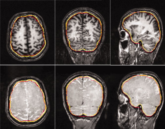
Segmentation of the inner skull surface: Comparison of the results using the bimodal T1‐ and PD‐MRI data set (in yellow) with the inner skull estimation approach using exclusively the T1‐MRI (in red) on underlying T1‐MRI (top row) and PD‐MRI (bottom row). Axial view (left), coronal view (middle), and sagittal view (right). [Color figure can be viewed in the online issue, which is available at www.interscience.wiley.com.]
Mesh Generation
A prerequisite for FE modeling is the generation of a mesh that represents the geometric and electric properties of the head volume conductor. To generate the mesh, we used the CURRY software [CURRY, 2000] to create a surface‐based tetrahedral tessellation of the four‐segmented compartments. The procedure exploited the Delaunay‐criterion, enabling the generation of compact and regular tetrahedra [Buchner et al., 1997; Wagner et al., 2000] and resulted in a FE model with N = 245,257 nodes and 1,503,357 tetrahedra elements.
The FE mesh is shown in Figure 2.
Figure 2.
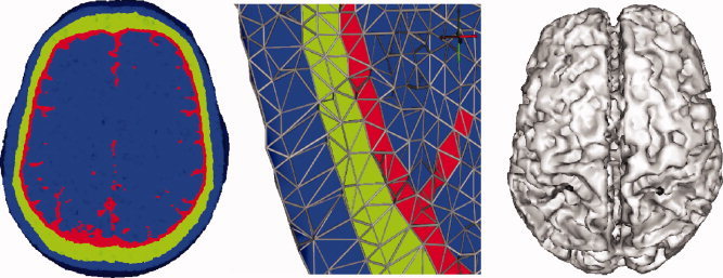
Four‐compartment (scalp, skull, CSF, and brain) realistic finite element head model. Cross section through the FE model without (left) and with (middle) visualization of the element edges. Right: The cortical influence source space. The somatosensory dipole sources are indicated by black dots. [Color figure can be viewed in the online issue, which is available at www.interscience.wiley.com.]
An influence source space that represented the brain gray matter in which dipolar source activities occur was extracted from a surface 2 mm beneath the outer cortical boundary. The influence space was tessellated with a 2‐mm mesh resulting in R = 21,383 influence nodes (shown in Fig. 2). Because the influence mesh is only a rough approximation of the real folded surface and does not appropriately model the cortical convolutions and deep sulci, no normal‐constraint was used, i.e., the dipole sources were not restricted to be oriented perpendicular to the source space. Instead, dipole sources in the three Cartesian directions were allowed.
Setup of the LRCE Simulation Studies
Simulation studies were carried out to validate the new LRCE approach. For the reference FE volume conductor, isotropic conductivity values of 0.33 (see [Haueisen, 1996] and references therein), 0.0132 [Lai et al., 2005], 1.79 [Baumann et al., 1997], and 0.33 S/m (see [Haueisen, 1996] and references therein) were assigned to the scalp, skull, CSF, and brain compartment of the FE model from section “mesh generation,” respectively. This led to a brain/skull conductivity ratio (four‐compartment head model) of 25 for the reference volume conductor. For the modeling of the EEG, 71 electrodes were placed on the reference volume conductor surface according to the international 10/10 EEG system. Two reference dipole sources were positioned on influence nodes in area 3b of the primary somatosensory cortex (SI) in both hemispheres, as shown in Figure 2 (right). Two source orientation scenarios were considered, in which both sources were either oriented quasi‐tangentially or quasi‐radially with regard to the inner skull surface. In both scenarios, the two sources were simultaneously activated using current densities of 100 nAm. Another experiment consisted of just a single source in the left SI with quasi‐tangential or quasi‐radial direction and a source strength of 100 nAm. Forward potential computations were carried out for the different scenarios using the direct FE approach as described in section “finite element method‐based forward problem.” Noncorrelated Gaussian noise was then added with SNRs of 40, 25, 20, and 15 dB (SNR(dB):= 20 log10(SNR) with  , where
  is the noisy signal and
  the noise at electrode i).
Figure 3 shows the potential maps for the two‐sources experiment for both orientation scenarios, the quasi‐tangential (top row) and the quasi‐radial orientations (bottom row) for different SNR values.
Figure 3.
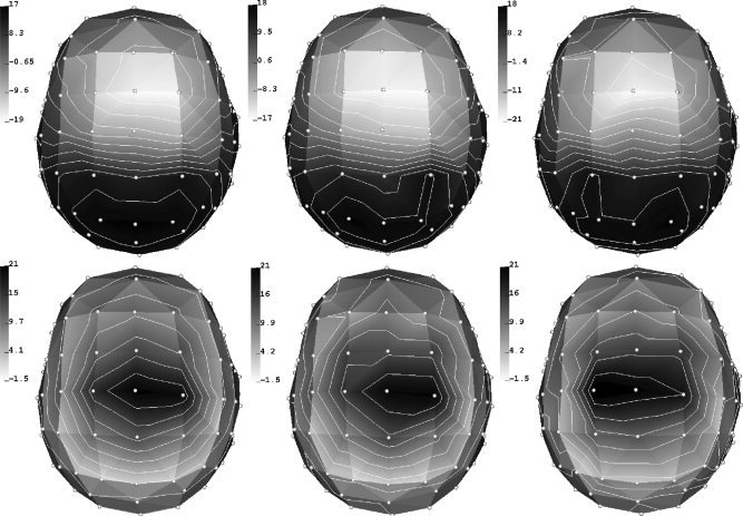
Simulated noisy (40, 25, and 20 dB from left to right) reference data for the two‐sources and two orientation scenarios in the reference volume conductor model. The top row shows the maps of the simultaneously active quasi‐tangentially oriented somatosensory sources, and the bottom row shows the maps of the simultaneously active quasi‐radially oriented sources. The potential maps are linearly interpolated (scale in μV) over the electrodes (white spheres). White lines indicate isopotentials.
For the SA optimization, the source space from section “mesh generation” was used as the influence space. A very slow cooling schedule with the cooling rate f t of 0.99 was applied to make sure that the search reached the global minimum of the cost function. The localization error was defined as the Euclidian distance between the somatosensory reference source locations and the inversely fitted ones resulting from the LRCE. The residual variance ν of the goal function was calculated as the percentile misfit between the noisy reference potential and the fitted potential that was computed from the fitted source parameters and conductivities. The explained variance shown in the result tables is 100% − ν.
SEP Measurement
We measured SEP data to apply our LRCE approach to real empirical EEG data. Tactile somatosensory stimuli were presented to the right index finger of the subject from section “registration and segmentation of MR images” using a balloon diaphragm driven by bursts of compressed air. We compensated for the delay between the electrical trigger and the arrival of the pressure pulse at the balloon diaphragm as well as the delay caused by the inertia of the pneumatic stimulation device (half‐way displacement of the membrane), together 52 ms in our measurements. Following standard practice [Mertens and Lütkenhöner, 2000], the stimuli were presented at 1 Hz (±10% variation to avoid habituation effects). A 63‐channel EEG (10% system) recorded the raw time signals for the SEP study. Two electrooculography (EOG) electrodes were furthermore used for horizontal and vertical eye movement control. The collection protocol consisted of three runs of 10 min each EEG data with a sampling rate of 1,200 samples/s using a real‐time low‐pass filter of 0–300 Hz. The BESA software [BESA, 2007] was then used for a rejection of noise‐contaminated epochs (e.g., epochs containing eye movements detected by means of the EOG channels) and for averaging the noncontaminated epochs within each run (83% of 601 epochs for run 1, 90% of 605 epochs for run 2, and 89% of 602 epochs for run 3). To optimize the SNR, the SEP data were furthermore averaged over the 1,579 noncontaminated epochs of the three runs. The data were measured with FCz as reference electrode. The baseline‐corrected (from −35 to 0 ms prestimulus) averaged EEG dataset was filtered using a fourth order butterfly digital filter with a bandwidth of 0.1–45 Hz. When using the prestimulus interval between −20 and 0 ms for the determination of the noise level and the peak of the first tactile component at 35.3 ms as the signal, we achieved a SNR of 24 dB. Finally, by means of a channel‐selection procedure (exclusion of 20 ipsilateral electrodes with poor SNR), we were able to even increase the SNR to 26.4 dB.
A butterfly‐ and a position‐plot of the SEP data are shown in Figure 4.
Figure 4.
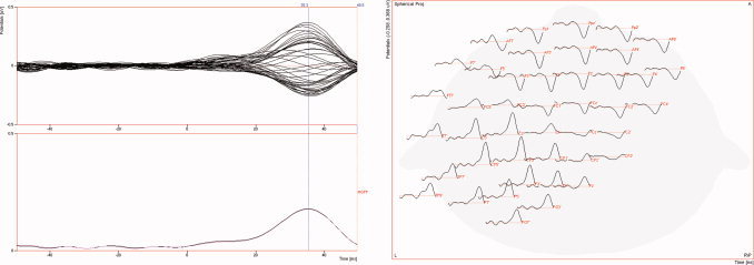
First tactile SEP component at the 43 selected electrodes. Selection was performed to optimize the SNR. Butterfly (left) and position plot (right). [Color figure can be viewed in the online issue, which is available at www.interscience.wiley.com.]
Computing Platform
All simulations and evaluations ran on a Linux‐PC with an Intel Pentium 4 processor (3.2 GHz) using the SimBio software environment (SimBio, 2008).
RESULTS
LRCE Simulation Studies
Simultaneous reconstruction of brain and skull conductivity and a pair of somatosensory sources
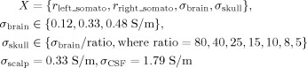
We performed the LRCE procedure as described in section “low‐resolution conductivity estimation” with an inverse two‐dipole fit on the discrete influence space, while additionally allowing skull and brain conductivity to vary as free discrete optimization parameters. The permitted brain conductivities (σbrain) were 0.12, 0.33 [Haueisen, 1996], and 0.48 S/m. For each brain conductivity, the skull conductivity (σskull) was allowed to vary so as to achieve brain/skull ratios (four‐compartment head model) of 80, 40, 25, 15, 10, 8, and 5. The CSF conductivity remained fixed at 1.79 S/m [Baumann et al., 1997] and the scalp conductivity at 0.33 S/m [Fuchs et al., 1998; Haueisen, 1996; Huiskamp et al., 1999]. Because of the fixed conductivities, possible problems are avoided that are due to the ambiguity between source strength and overall conductivity. This resulted in a total of 21 conductivity configurations.
 |
Following Eq. (4), the total number of possible source and conductivity configurations in this simulation was thus ∼4.8 billion.
Table I contains the LRCE source localization and conductivity estimation results for the simulated reference EEG data, and Table II the LRCE reconstruction errors in the corresponding dipole moments. As the tables show, besides appropriately reconstructing both sources, the LRCE was able to accurately select the reference conductivity values of the brain and the skull compartment in the cases of no noise (max. errors: 0 mm loc., 0° orientation, 0% magnitude) and low noise (40 dB, max. errors: 3 mm loc., 6° orientation, 18% magnitude). However, for the noisier data with an SNR of 25 or lower, neither the somatosensory sources nor the brain and the skull conductivity values could be reconstructed correctly. The wall clock time for setting up the global lead field matrix Λ was 199 min. When averaging over all noise configurations and source orientation scenarios, the SA needed about 17 h of computation time for finding the global optimum (results indicated in Tables I and II). Much of it was access‐time to the global lead field matrix within the LRCE procedure.
Table I.
Results of the LRCE algorithm for a simultaneous reconstruction of the brain and the skull conductivity together with two dipole sources
| Reference SEP | Localization error (mm) | Estimated conductivity | Goal function | ||
|---|---|---|---|---|---|
| Right dipole | Left dipole | σbrain (S/m) | σbrain/σskull | Expl. var. (%) | |
| (a) Tangential reference sources | |||||
| Noise free | 0 | 0 | 0.33 | 25 | 100 |
| 40 dB | 2.2 | 2.2 | 0.33 | 25 | 99.8 |
| 25 dB | 3.2 | 10.7 | 0.12 | 10 | 99.0 |
| 20 dB | 13.4 | 10.4 | 0.48 | 15 | 97.4 |
| (b) Radial reference sources | |||||
| Noise free | 0 | 0 | 0.33 | 25 | 100 |
| 40 dB | 3.0 | 3.0 | 0.33 | 25 | 99.4 |
| 25 dB | 6.4 | 7.4 | 0.48 | 25 | 96.6 |
| 20 dB | 5.2 | 12.5 | 0.48 | 25 | 92.8 |
Underlying reference sources in the somatosensory cortex had (a) tangential and (b) radial orientation. Part I: Estimated conductivity and, rounded to 1 digit after the decimal point, localization error (mm) and explained variance to the data (%).
Table II.
Results of the LRCE algorithm for a simultaneous reconstruction of the brain and the skull conductivity together with two dipole sources
| Reference SEP | Tangential | Radial | ||
|---|---|---|---|---|
| Right dipole | Left dipole | Right dipole | Left dipole | |
| (a) Orientation error (in degree) | ||||
| Noise free | 0 | 0 | 0 | 0 |
| 40 dB | 6 | 3 | 2 | 5 |
| 25 dB | 16 | 30 | 10 | 16 |
| 20 dB | 17 | 12 | 9 | 14 |
| (b) Magnitude error (in %) | ||||
| Noise free | 0 | 0 | 0 | 0 |
| 40 dB | 15 | 18 | 17 | 12 |
| 25 dB | 54 | 1 | 10 | 25 |
| 20 dB | 102 | 34 | 19 | 54 |
Part II: Error (rounded to integer numbers) in dipole (a) orientation (in degree) and (b) magnitude (in %).
Simultaneous reconstruction of brain and skull conductivity and a single source in the left somatosensory cortex
In the second simulation, we first generated noise‐free and noisy reference data for a single dipole source in the left SI and then performed a single dipole fit with skull and brain conductivity as two additional free optimization parameters in the LRCE. We used the same scalp, skull, CSF, and brain conductivity values as in the previous simulation:
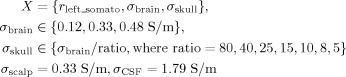 |
The number of possible source and conductivity configurations was 449 K [Eq. (4)].
As shown in Tables III and IV, the conductivities were accurately estimated for reference data with 40 and 25 dB SNR, and the source reconstruction errors were very low (max. errors for 40 dB: 0 mm loc., 1° orientation, 1% magnitude; max. errors for 25 dB: 2 mm loc., 4° orientation, 2% magnitude). For 20 dB, the skull to brain conductivity ratio was still correct and the source reconstruction was still acceptable (max. errors: 4 mm loc., 9° orientation, 12% magnitude), but the brain conductivity was no longer correctly reconstructed. Still higher noise levels led to unacceptable results. Like in section “simultaneous reconstruction of brain and skull conductivity and a pair of somatosensory sources,” the wall clock time for setting up the global lead field matrix Λ was 199 min. When averaging over all noise configurations and source orientation scenarios, the LRCE procedure took about 1.3 min of computation time for finding the global optimum (results indicated in Tables III and IV).
Table III.
Results of the LRCE algorithm for a simultaneous reconstruction of the brain and the skull conductivity together with a single dipole source
| Reference SEP | Localization error (mm) | Estimated conductivity | Goal function | |
|---|---|---|---|---|
| σbrain (S/m) | σbrain/σskull | Expl. var. (%) | ||
| (a) Tangential reference source | ||||
| Noise free | 0 | 0.33 | 25 | 100 |
| 40 dB | 0 | 0.33 | 25 | 99.9 |
| 25 dB | 2.2 | 0.33 | 25 | 96.7 |
| 20 dB | 4.1 | 0.48 | 25 | 95.8 |
| 15 dB | 9.4 | 0.12 | 25 | 83.4 |
| (b) Radial reference source | ||||
| Noise free | 0 | 0.33 | 25 | 100 |
| 40 dB | 0 | 0.33 | 25 | 99.9 |
| 25 dB | 2.2 | 0.33 | 25 | 98.4 |
| 20 dB | 4.1 | 0.12 | 25 | 90.0 |
| 15 dB | 10.8 | 0.48 | 10 | 79.0 |
The underlying reference source in the somatosensory cortex had (a) tangential and (b) radial orientation. Part I: Estimated conductivity and, rounded to 1 digit after the decimal point, localization error (mm) and explained variance to the data (%).
Table IV.
Results of the LRCE algorithm for a simultaneous reconstruction of the brain and the skull conductivity together with a single dipole source
| Reference SEP | Tangential | Radial |
|---|---|---|
| (a) Orientation error (in degree) | ||
| Noise free | 0 | 0 |
| 40 dB | 1 | 0 |
| 25 dB | 3 | 4 |
| 20 dB | 9 | 1 |
| 15 dB | 6 | 25 |
| (b) Magnitude error (in %) | ||
| Noise free | 0 | 0 |
| 40 dB | 0 | 1 |
| 25 dB | 2 | 1 |
| 20 dB | 7 | 12 |
| 15 dB | 40 | 9 |
Part II: Error (rounded to integer numbers) in dipole (a) orientation (in degree) and (b) magnitude (in %).
Simultaneous reconstruction of the brain/skull conductivity ratio and a pair of somatosensory sources
We carried out a third simulation, in which only skull conductivity was allowed to vary with fixed conductivity values for brain (0.33 S/m), scalp (0.33 S/m), and CSF (1.79 S/m). The brain/skull conductivity ratio (four‐compartment model) was chosen as follows.
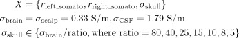 |
The total number of possible source and conductivity configurations for this scenario was 1.6 billion [Eq. (4)].
As shown in Tables V and VI, for both source orientation scenarios, the LRCE estimated the skull conductivity correctly down to a 20 dB SNR, while reasonable source reconstructions were only achieved down to 25 dB (<8 mm loc., <16° orientation, <15% magnitude). The LRCE reconstruction failed to give acceptable results for both the brain/skull conductivity ratio (four‐compartment model) and the source reconstructions only at an SNR of 15 dB or lower. The wall clock time for setting up the global lead field matrix Λ was 66 min. When averaging over all noise configurations and source orientation scenarios, the LRCE procedure took about 451 min of computation time for finding the global optimum (results indicated in Tables V and VI). Again, much of it was access‐time to the global lead field matrix within the LRCE procedure.
Table V.
Results of the LRCE algorithm for a simultaneous reconstruction of the brain/skull conductivity ratio together with two dipole sources
| Reference SEP | Localization error (mm) | Estimated | Goal function | |
|---|---|---|---|---|
| Right dipole | Left dipole | σbrain/σskull | Expl. var.(%) | |
| (a) Tangential reference sources | ||||
| Noise free | 0 | 0 | 25 | 100 |
| 40 dB | 2.2 | 2.2 | 25 | 99.8 |
| 25 dB | 2.0 | 3.3 | 25 | 99.0 |
| 20 dB | 6.0 | 5.9 | 25 | 97.4 |
| 15 dB | 17.6 | 41.1 | 15 | 64.3 |
| (b) Radial reference sources | ||||
| Noise free | 0 | 0 | 25 | 100 |
| 40 dB | 3.0 | 3.0 | 25 | 99.4 |
| 25 dB | 7.4 | 7.5 | 25 | 96.6 |
| 20 dB | 5.2 | 10.7 | 25 | 92.7 |
| 15 dB | 24.6 | 13.2 | 5 | 89.1 |
Underlying reference sources in the somatosensory cortex had (a) tangential and (b) radial orientations. Part I: Estimated conductivity and, rounded to 1 digit after the decimal point, localization error (mm) and explained variance to the data (%).
Table VI.
Results of the LRCE algorithm for a simultaneous reconstruction of the brain/skull conductivity ratio together with two dipole sources
| Reference SEP | Tangential | Radial | ||
|---|---|---|---|---|
| Right dipole | Left dipole | Right dipole | Left dipole | |
| (a) Orientation error (in degree) | ||||
| Noise free | 0 | 0 | 0 | 0 |
| 40 dB | 6 | 3 | 2 | 5 |
| 25 dB | 2 | 6 | 11 | 16 |
| 20 dB | 10 | 10 | 7 | 15 |
| 15 dB | 9 | 24 | 8 | 6 |
| (b) Magnitude error (in %) | ||||
| Noise free | 0 | 0 | 0 | 0 |
| 40 dB | 15 | 18 | 17 | 12 |
| 25 dB | 8 | 8 | 15 | 7 |
| 20 dB | 26 | 1 | 6 | 40 |
| 15 dB | 21 | 14 | 41 | 68 |
Part II: Error (rounded to integer numbers) in dipole (a) orientation (in degree) and (b) magnitude (in %).
Simulation with a fixed conductivity and a pair of somatosensory sources
In a last simulation, volume conductors with fixed skull conductivity values from the set of σskull from section “simultaneous reconstruction of the brain/skull conductivity ratio and a pair of somatosensory sources” were used. For these fixed volume conductors, only the two somatosensory sources were reconstructed on the discrete influence space using the SA optimizer with reference EEG data at an SNR of 25 dB.
The results in Table VII show the effects of an erroneous choice of the brain/skull conductivity ratio (four‐compartment model) (80, 40, 15, 10, 8, 5) on the localization accuracy in comparison to the localization errors caused just by the addition of noise when using the correct brain/skull ratio (four‐compartment model) of 25. Incorrect skull conductivity within the source localization caused large localization errors. As expected, the correct skull conductivity (σbrain/σskull = 25) gave the smallest localization errors and the highest explained variance for both source orientation scenarios.
Table VII.
Localization error (mm) and explained variance to the data (%) rounded to 1 digit after the decimal point for a fixed brain/skull conductivity ratio using the simulated reference SEP data with an SNR of 25 dB
| σbrain/σskull | Tangential | Radial | ||||
|---|---|---|---|---|---|---|
| Right (mm) | Left (mm) | Expl. var. (%) | Right (mm) | Left (mm) | Expl. var. (%) | |
| 80 | 12.7 | 10.8 | 98.6 | 13.1 | 15.2 | 95.9 |
| 40 | 3.8 | 11.2 | 99.0 | 7.5 | 8.3 | 96.4 |
| 25 | 2.0 | 3.3 | 99.0 | 7.4 | 7.5 | 96.5 |
| 15 | 3.2 | 10.7 | 99.0 | 6.8 | 10.0 | 96.5 |
| 10 | 2.2 | 10.7 | 99.0 | 7.1 | 10.9 | 96.3 |
| 8 | 7.1 | 10.7 | 98.7 | 10.1 | 10.8 | 96.1 |
| 5 | 3.3 | 20.5 | 98.9 | 10.0 | 18.1 | 96.3 |
Application of LRCE to the SEP Data
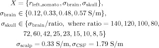
In a last examination, the new LRCE algorithm was applied to the post stimulus P35 component of the averaged SEP data at the peak latency of 35.3 ms as indicated in Figure 4. The detailed four‐compartment (scalp, skull, CSF, and brain) FE model with improved segmentation of skull and CSF geometry described in section “mesh generation” was used as the volume conductor. Because of the limiting SNR of 26.4 dB for the SEP data and based on our simulation results from section “LRCE simulation studies,” we focused on the simultaneous reconstruction of the contralateral somatosensory P35 source in combination with the estimation of both the brain and the skull conductivities. Accordingly, we assigned fixed isotropic conductivities to CSF (1.79 S/m) [Baumann et al., 1997] and scalp (0.33 S/m) [Fuchs et al., 1998; Haueisen et al., 1996; Huiskamp et al., 1999]. Again, the source space from section “mesh generation” was used as the influence space for SA optimization together with brain/skull conductivity ratios (four‐compartment head model) of 140, 120, 100, 80, 72, 60, 42, 25, 23, 15, 10, 8, and 5 ([Hoekema et al., 2003], who claimed ratios of 10 up to only 4).
 |
The total number of possible source and conductivity configurations was 1,026 K.
Applying the LRCE approach resulted in the contralateral somatosensory source shown in Figure 5, in the brain conductivity of 0.48 S/m and in a skull conductivity of 0.004 S/m, with an explained variance of 99%. Although the value of skull conductivity is close to what is generally used in three‐compartment head model‐based source analysis, with 0.48 S/m, the value of brain conductivity is higher than the commonly used (in three‐compartment approaches) value of 0.33 S/m (e.g., [Buchner et al., 1997; de Munck and Peters, 1993; Fuchs et al., 1998; Huiskamp et al., 1999; Waberski et al., 1998; Zanow, 1997]). The estimated brain conductivity is however still in the range of brain conductivity values that were determined by others (e.g., the value of 0.57 S/m for subject 1 in Goncalves et al. [2003a], 0.43 S/m for subject 5 in Goncalves et al. [2003b], 0.42 S/m for subject S2 in Baysal and Haueisen [2004]). The wall clock time for setting up the global lead field matrix Λ was about 315 min and the LRCE procedure took about 10 min of computation time.
Figure 5.
Source reconstruction result for the first tactile SEP component at the peak latency of 35.3 ms. [Color figure can be viewed in the online issue, which is available at www.interscience.wiley.com.]
DISCUSSION AND CONCLUSIONS
We developed a LRCE procedure to individually optimize a volume conductor model from a human head with regard to both geometry and tissue conductivities. We only exploited SEP data and a combined T1‐/PD‐MRI dataset for the construction of a four‐tissue (scalp, skull, CSF, brain) volume conductor FE model. The proposed procedure is safe and noninvasive, and EEG laboratories should most often have access to such datasets, so that no additional hard‐ and software is needed, in contrast to, e.g., approaches based on EIT [Gonçalves et al., 2003b]. For the FE model, a special focus was on an improved modeling of the skull shape and thickness and on the highly conducting CSF compartment [Baumann et al., 1997; Huiskamp et al., 1999; Ramon et al., 2004; Rullmann et al., 2009; Wendel et al., 2008; Wolters et al., 2006]. Obtaining accurate skull geometry is important because changes in skull conductivity are known to be closely related to changes in its compartmental thickness. The correction for geometry errors in modeling the skull compartment were furthermore shown to be essential for the measurement of skull conductivity [Gonçalves et al., 2003b]. Although other authors have used parameter estimation in continuous parameter space with local optimization algorithms [Fuchs et al., 1998; Gutiérrez et al., 2004; Vallaghe et al., 2007, Zhang et al., 2006], we propose the combination of a discrete low‐resolution parameter estimation with a global optimization method applied to realistic four‐compartment geometry to better take into account the limited SNR of real SEP or AEP measurement data. Because the cost function is shallow [Gonçalves et al., 2003a], the proposed procedure using realistic FE volume conductor modeling and SA optimization for approximating the global minimum in acceptable computation time is important. Although other authors used three‐compartment BE [Fuchs et al., 1998; Gonçalves et al., 2003a; Plis et al., 2007; Vallaghe et al., 2007] or FE models [Zhang et al., 2006] (in the latter, additionally to the three layers scalp, skull, and brain, a low‐conducting silastic ECoG grid was modeled) for conductivity estimation, we additionally model the CSF with a fixed conductivity of 1.79 S/m [Baumann et al., 1997], not only because its modeling was shown to have a large impact on forward and inverse source analysis [Baumann et al., 1997; Huang et al., 1990; Ramon et al., 2004; Rullmann et al., 2009; Wendel et al., 2008; Wolters et al., 2006], but also to avoid the problem of the ambiguity between source strength and overall conductivity. In Rullmann et al. [2009], noninvasive EEG source analysis was validated by means of intracranial EEG measurements, and it was shown that ignoring the CSF by means of the commonly used three‐compartment realistically shaped volume conductor led to spurious reconstruction results. Plis et al. [2007] derived a lower Cramer‐Rao bound for the simultaneous estimation of source and skull conductivity parameters in a sphere model for dipoles whose locations were not constraint within the inner sphere volume. Because source depth and skull conductivity are closely related, their final result was that it is impossible to simultaneously reconstruct both source and skull conductivity parameters from measured surface EEG data in the sphere model. This is an important theoretical result; however, there are strong differences to our study. Our study, as well as the symmetric BEM study of Vallaghe et al. [2007], used a cortex constraint, i.e., sources were only allowed on a surface. We furthermore used a realistic four‐compartment FE model of the head instead of the spherical volume conductor model that was used for the derivation of the Cramer‐Rao bounds in Plis et al. [2007], and we fixed the conductivity of the CSF compartment in our analysis to the value measured by Baumann et al. [1997]. We only allowed a user‐given discrete set of some few (“low resolution”) possible conductivity values for those tissues where conductivity measurements or other methods resulted in different estimates. We propose to only apply the presented LRCE algorithm to EEG data where the underlying sources are rather simple and where very good SNR ratios can be achieved like, e.g., SEP and/or AEP data.
In the first simulation studies, we evaluated the LRCE algorithm in EEG simulations for its ability to determine both the brain and the skull tissue conductivities together with the reconstruction of one and two reference sources. At relatively low noise levels (down to 25 dB SNR in the single‐source scenario and down to 40 dB SNR in the two‐source scenario), the LRCE resulted in acceptable reconstruction errors for the reference sources and correctly estimated reference tissue conductivities, whereas results became unstable when further increasing the noise. We also set up a simulation for the reconstruction of the skull to brain conductivity ratio (four‐compartment model) together with two sources in which results were reasonable (correct skull/brain conductivity ratio, max. source reconstruction errors: <8 mm loc., <16° orientation, <15% magnitude) down to noise levels of 25 dB. We found in our simulations that the most accurate source reconstructions were associated with the correctly estimated conductivities (or conductivity ratio) and, moreover, that assuming an incorrect conductivity ratio had a profoundly negative effect on the source reconstruction accuracy.
In a last examination, we applied the LRCE to measured tactile SEP data with the focus on estimating both the brain and the skull conductivity. With an SNR of 26.4 dB, the data were in the noise range of the second simulation study, which was based on a single equivalent current dipole model. As shown in numerous studies [Hari and Forss, 1999; Mertens and Lütkenhöner, 2000], this source model is adequate because the early SEP component arises from area 3b of the primary SI contralateral to the side of stimulation. Our explained variance to the measured data of about 99% for this source model further supports our choice. The results from the LRCE analysis were a brain conductivity of 0.48 S/m and a skull conductivity of 0.004 S/m. Although this skull conductivity corresponds to the traditional value in the literature [Buchner et al., 1997; de Munck and Peters, 1993; Fuchs et al., 1998], we found the brain to have a lower resistance than generally assumed in three‐compartment head modeling approaches (e.g., [Buchner et al., 1997; de Munck and Peters, 1993; Fuchs et al., 1998; Huiskamp et al., 1999; Waberski et al., 1998; Zanow, 1997]), but it is however still in the range of brain conductivity values that were determined by others (e.g., the value of 0.57 S/m for subject 1 in Goncalves et al. [2003a], 0.43 S/m for subject 5 in Goncalves et al. [2003b], 0.42 S/m for subject S2 in Baysal and Haueisen [2004]). Many recent articles have focused on the brain/skull conductivity ratio and a large variability of results has been reported for this value including 80 [Homma et al., 1995], 72 [Gonçalves et al., 2003a], 42 [Gonçalves et al., 2003b], 25 ± 7 [Lai et al., 2005], 23 [Baysal and Haueisen, 2004], 18.7 ± 2.1 [Zhang et al., 2006], 15 [Oostendorp et al., 2000], and 8 [Hoekema et al., 2003]. Because of the higher conductivity of the brain, with an estimated brain to skull conductivity ratio of 120 (in a four‐compartment head model), our LRCE result is larger than the commonly used ratio of 80 (in a three‐compartment model) [Homma et al., 1995; Rush and Driscoll, 1968, 1969]. Note that, in contrast to the studies using three‐compartment modeling [Baysal and Haueisen, 2004; Gonçalves et al., 2003a, b; Homma et al., 1995; Lai et al., 2005; Oostendorp et al., 2000; Vallaghe et al., 2007], our approach took the highly conducting CSF compartment into account. It is well known that an increased conductivity of the brain compartment leads to a decreased potential magnitude at the head surface, whereas an increased conductivity of the CSF leads to an increased potential magnitude. Because we modeled the CSF with the value of 1.79 S/m as measured by Baumann et al. [1997] (i.e., a more than a factor of 5.4 higher value than the commonly used 0.33 S/m in the three‐compartment models), an increased conductivity value for the brain compartment has to be expected in the four‐compartment model. Our brain‐to‐skull conductivity ratio (in a four‐compartment model) of 120 thus has to be interpreted in light of the aforementioned considerations.
With regard to computational complexity (or feasibility in daily routine), former FE approaches, which were not based on the presented transfer matrix approach, and on algebraic multigrid FE solver methods would have needed weeks or even months for the computation of a single lead field matrix for a single conductivity configuration, so that the proposed FE‐based LRCE approach would not have been feasible in practice. In Buchner et al. [1997], the computation of a single lead field matrix for an FE mesh with 18,322 nodes and an influence space with 2,914 nodes took roughly a week of computation time. Waberski et al. [1998] used an FE model with 10,713 nodes and concluded that improved headmodeling by finer discretization and more accurate representation of the conductivities are necessary, and parallel computing is needed to speed up the computation. The FE head model of Zhang et al. [2006] for the estimation of the in vivo brain‐to‐skull conductivity ratio had 29,858 nodes. For our presented LRCE approach, the underlying FE mesh had a resolution of 245,257 FE nodes, which was necessary not only to appropriately model the CSF compartment, and our influence space had 21,383 nodes. Furthermore, our LRCE algorithm does not only need to precompute a single lead field matrix, but as many lead field matrices as we have combinations of user‐given conductivity values for the different tissue compartments as indicated by the global lead field matrix in Eq. (3). Still the presented LRCE approach, as indicated by means of the computation times in section “results” (measured on a single processor machine, see section “computing platform”), is practically feasible in daily routine with a computational amount of work in the range of some few hours.
The following limitations of our study are important: The data of a single subject are not representative for other subjects because we have to be aware of larger inter‐ and intrasubject variability. The variability can be related to age, diseases, environmental factors, and personal constitution as shown in animal studies [Crile et al., 1922] and as shown for humans by means of the large discrepancy in the estimated brain‐to‐skull conductivity ratios (in three‐compartment models) between 80 [Homma et al., 1995; Rush and Driscoll, 1968, 1969] and 15 [Oostendorp et al., 2000]. Further simulation studies should be carried out that consider noise from, e.g., the prestimulus interval of evoked potential measurements. The presented LRCE procedure has to be automatized to allow a statistical evaluation of possible errors and instabilities at different noise levels. We are currently working on such investigations for a combined SEP/SEF‐LRCE approach. The influence of a realistic extent of an active cortical patch on our focal source‐based LRCE method should be evaluated, and its sensitivity to biological noise (nonmodeled “noise” current sources in the brain) has to be examined. The performance of other global optimization approaches such as genetic algorithms [Kjellström, 1996] should be compared with the approach chosen here, and higher FE resolutions have to be used to avoid geometry representation problems in areas where, e.g., the CSF or the skull compartments are very thin using, e.g., 1‐mm hexahedra FE modeling as described in Rullmann et al. [2009].
These results illustrate the feasibility of building an optimized volume conductor model with regard to both geometry and conductivity. As we have formulated it, such a study requires accurate head geometry, in this case from both T1‐ and PD‐weighted MRI (or T2‐MRI) and cortical constraints on the sources. The highly conducting CSF should not be neglected in the headmodel [Baumann et al., 1997; Huang et al., 1990; Ramon et al., 2004; Rullmann et al., 2009; Wendel et al., 2008; Wolters et al., 2006] and our procedure takes this compartment into account. By obtaining SEP data, which allows independent reconstruction of the underlying bioelectric source, it is then possible to estimate the optimal conductivities for the individual subject using the proposed LRCE approach in highly realistic FE models, provided that the data have a sufficient SNR ratio. Note that one might also think of simultaneously evaluating SEP data of different finger or toes ([Vallaghe et al., 2007], e.g., used left‐ and right‐hand index finger SEP data). A related finding from this study is, there is a trade off between the number of independent parameters that can be determined and the complexity of the assumed source model. The specific trade off point is also strongly influenced by the quality of the measured electric potentials. Thus, the number of parameters that can be dependably estimated is a function of both the signal quality and the number and quality of a priori knowledge about, for example, the source location or orientation through a combination with fMRI or anatomical and/or functional arguments (e.g., a strong restriction of the source location to anatomically and physiologically reasonable areas close to the somatosensory SI area). In this context, others have suggested that by including MEG data in the scheme [Fuchs et al., 1998; Huang et al., 2007], it will be possible to improve stability considerably. We note that our approach differs from their procedures with regard to both head modeling and conductivity optimization.
The success of the conductivity optimization approach and the more general advantages of customized geometric models suggest a procedure for clinical applications. First of all, one could use SEP and/or AEP data with high SNR together with T1‐ and PD‐MR (or T2‐MR) images from the patient to construct a model that would be optimized for both geometric accuracy and individual conductivity values. With this volume conductor model in place, recorded potentials from more complex and clinically interesting sources could drive the inverse solution and source analysis.
A better approximation to the real volume conductor using the proposed LRCE method is an important step toward simultaneous EEG/MEG source analysis. Combining EEG and MEG modalities compensates each others disadvantages, i.e., poor sensitivity of MEG to radial sources and the much stronger conductivity dependency of EEG [Fuchs et al., 1998; Huang et al., 2007]. Using combined SEP/SEF in combination with T1‐ and PD‐MRI (or T2‐MRI) should further stabilize the application of the presented LRCE method for the estimation of tissue conductivities. For the quasi‐tangentially oriented P35 somatosensory source, MEG‐SEF data can be exploited to strongly restrict the source location and especially its depth as shown, e.g., in [Fuchs et al., 1998; Huang et al., 2007], so that the resolution of the proposed LRCE method with regard to the conductivities of the different compartments could be increased. With such data in hand, the presented LRCE method using FE volume conductor modeling might also contribute to the estimation of conductivity values for further compartments like the scalp or of anisotropy ratios in the skull and brain compartments [Haueisen et al., 2002; Marin et al., 1998; Rullmann et al., 2009; Wolters et al., 2006].
Acknowledgements
The authors thank the anonymous reviewers for their helpful critics and comments that significantly improved our manuscript.
REFERENCES
- Baumann S,Wozny D,Kelly S,Meno F ( 1997): The electrical conductivity of human cerebrospinal fluid at body temperature. IEEE Trans Biomed Eng 44: 220–223. [DOI] [PubMed] [Google Scholar]
- Baysal U,Haueisen J ( 2004): Use of a priori information in estimating tissue resistivities‐application to human data in vivo. Physiol Meas 25: 737–748. [DOI] [PubMed] [Google Scholar]
- Bertrand O,Thévenet M,Perrin F ( 1991): 3D finite element method in brain electrical activity studies In: Nenonen J,Rajala H, Katila T, editors. Biomagnetic Localization and 3D Modelling. Report of the Department of Technical Physics. Finland: Helsinki University of Technology; pp 154–171. [Google Scholar]
- BESA ( 2007): Brain electric source analysis. Available at: http://www.besa.de.
- Buchner H,Knoll G,Fuchs M,Rienäcker A,Beckmann R,Wagner M,Silny J,Pesch J ( 1997): Inverse localization of electric dipole current sources in finite element models of the human head. Electroencephalogr Clin Neurophysiol 102: 267–278. [DOI] [PubMed] [Google Scholar]
- Crile GW,Hosmer HR,Rowland AF ( 1922): The electrical conductivity of animal tissues under normal and pathological conditions. Am J Physiol 60: 59–106. [Google Scholar]
- Cuffin BN ( 1996): EEG localization accuracy improvements using realistically shaped head model. IEEE Trans Biomed Eng 43: 299–303. [DOI] [PubMed] [Google Scholar]
- CURRY ( 2000): Current reconstruction and imaging. Available at: http://www.neuro.com.
- de Munck J ( 1992): A linear discretization of the volume conductor boundary integral equation using analytically integrated elements. IEEE Trans Biomed Eng 39: 986–990. [DOI] [PubMed] [Google Scholar]
- de Munck J,Peters M ( 1993): A fast method to compute the potential in the multi sphere model. IEEE Trans Biomed Eng 40: 1166–1174. [DOI] [PubMed] [Google Scholar]
- Fuchs M,Wagner M,Wischmann H,Köhler T,Theißen A,Drenckhahn R,Buchner H ( 1998): Improving source reconstructions by combining bioelectric and biomagnetic data. Electroencephalogr Clin Neurophysiol 107: 93–111. [DOI] [PubMed] [Google Scholar]
- Geddes L,Baker L ( 1967): The specific resistance of biological materials. A compendium of data for the biomedical engineer and physiologist. Med Biol Eng 5: 271–293. [DOI] [PubMed] [Google Scholar]
- Geman S,Geman D ( 1984): Stochastic relaxation, Gibbs distribution and the Bayesian restoration of images. IEEE Trans Pattern Anal Mach Intell 6: 721–741. [DOI] [PubMed] [Google Scholar]
- Gençer NG,Acar CE ( 2004): Sensitivity of EEG and MEG measurements to tissue conductivity. Phys Med Biol 49: 701–717. [DOI] [PubMed] [Google Scholar]
- Gerson J,Vardenas VA,Fein G ( 1994): Equivalent dipole parameter estimation using simulated annealing. Electroencephalogr Clin Neurophysiol 92: 161–168. [DOI] [PubMed] [Google Scholar]
- Gonçalves S,de Munck JC,Verbunt JPA,Heethaar RM,da Silva FHL ( 2003a): In vivo measurement of the brain and skull resistivities using an EIT‐based method and the combined analysis of SEF/SEP data. IEEE Trans Biomed Eng 50: 1124–1128. [DOI] [PubMed] [Google Scholar]
- Gonçalves S,de Munck JC,Jeroen PA,Heethaar RM,da Silva FLL ( 2003b): In vivo measurement of the brain and skull resistivities using an EIT‐based method and realistic models for the head. IEEE Trans Biomed Eng 50: 754–767. [DOI] [PubMed] [Google Scholar]
- Gutiérrez D,Nehorai A,Muravchik CH ( 2004): Estimating brain conductivities and dipole source signals with EEG arrays. IEEE Trans Biomed Eng 51: 2113–2122. [DOI] [PubMed] [Google Scholar]
- Hallez H,Vanrumste B,Hese PV,D'Asseler Y,Lemahieu I,de Walle RV ( 2005): A finite difference method with reciprocity used to incorporate anisotropy in electroencephalogram dipole source localization. Phys Med Biol 50: 3787–3806. [DOI] [PubMed] [Google Scholar]
- Hämäläinen M,Sarvas J ( 1989): Realistic conductivity geometry model of the human head for interpretation of neuromagnetic data. IEEE Trans Biomed Eng 36: 165–171. [DOI] [PubMed] [Google Scholar]
- Haneishi H,Ohyama N,Sekihara K,Honda T ( 1994): Multiple current dipole estimation using simulated annealing. IEEE Trans Biomed Eng 41: 1004–1009. [DOI] [PubMed] [Google Scholar]
- Hari R,Forss N ( 1999): Magnetoencephalography in the study of human somatosensory cortical processing. Philos Trans R Soc Lond B Biol Sci 354: 1145–1154. [DOI] [PMC free article] [PubMed] [Google Scholar]
- Haueisen J ( 1996): Methods of numerical field calculation for neuromagnetic source localization. Ph.D. Thesis Shaker‐Verlag, Aachen, Germany; ISBN 3‐8265‐1691‐5.
- Haueisen J,Tuch D,Ramon C,Schimpf P,Wedeen V,George J,Belliveau J ( 2002): The influence of brain tissue anisotropy on human EEG and MEG. Neuroimage 15: 159–166. [DOI] [PubMed] [Google Scholar]
- Hoekema R,Wieneke GH,Leijten FSS,van Veelen CWM,van Rijen PC,Huiskamp GJM,Ansems J,van Huffelen AC ( 2003): Measurement of the conductivity of skull, temporarily removed during epilepsy surgery. Brain Topogr 16: 29–38. [DOI] [PubMed] [Google Scholar]
- Homma S,Musha T,Nakajima Y,Okamoto Y,Blom S,Flink R,Hagbarth KE ( 1995): Conductivity ratios of scalp‐skull‐brain model in estimating equivalent dipole sources in human brain. Neurosci Res 22: 51–55. [DOI] [PubMed] [Google Scholar]
- Huang JC,Nicholson C,Okada YC ( 1990): Distortion of magnetic evoked fields and surface potentials by conductivity differences at boundaries in brain tissue. Biophys J 57: 1155–1166. [DOI] [PMC free article] [PubMed] [Google Scholar]
- Huang M,Song T,Hagler D,Podgorny I,Jousmaki V,Cui L,Gaa K,Harrington DL,Dale A,Lee RR,Elman J,Hargren E ( 2007): A novel integrated MEG and EEG analysis method for dipolar sources. Neuroimage 37: 731–748. [DOI] [PMC free article] [PubMed] [Google Scholar]
- Huiskamp G,Vroeijenstijn M,van Dijk R,Wieneke G,van Huffelen A ( 1999): The need for correct realistic geometry in the inverse EEG problem. IEEE Trans Biomed Eng 46: 1281–1287. [DOI] [PubMed] [Google Scholar]
- Hütten S ( 1993): Über das asymptotische Verhalten von simulated annealing. Diplomarbeit in Mathematik Institut für Statistik und Wirtschaftsmathematik,RWTH Aachen. Available at: http://www.stochastik.rwth-aachen.de/.
- Kirkpatrick S,Gelatt CD Jr,Vecchi MP ( 1983): Optimization by simulated annealing. Science 220: 671–680. [DOI] [PubMed] [Google Scholar]
- Kjellström G ( 1996): Evolution as a statistical optimization algorithm. Evol Theory 11: 105–117. [Google Scholar]
- Kybic J,Clerc M,Abboud T,Faugeras O,Keriven R,Papadopoulo T ( 2005): A common formalism for the integral formulations of the forward EEG problem. IEEE Trans Med Imaging 24: 12–18. [DOI] [PubMed] [Google Scholar]
- Lai Y,van Drongelen W,Ding L,Hecox KE,Towle VL,Frim DM,He B ( 2005): Estimation of in vivo human brain‐to‐skull conductivity ratio from simultaneous extra‐ and intra‐cranial electrical potential recordings. Clin Neurophysiol 116: 456–465. [DOI] [PubMed] [Google Scholar]
- Lanfer B ( 2007): Validation and comparison of realistic head modeling techniques and application to tactile somatosensory evoked EEG and MEG data. Master Thesis in Physics,Institute of Biomagnetism and Biosignalanalysis, Westfälische Wilhelms‐Universität Münster.
- Latikka J,Kuume T,Eskola H ( 2001): Conductivity of living intracranial tissues. Phys Med Biol 46: 1611–1616. [DOI] [PubMed] [Google Scholar]
- Marin G,Guerin C,Baillet S,Garnero L,Meunier G ( 1998): Influence of skull anisotropy for the forward and inverse problem in EEG: Simulation studies using the FEM on realistic head models. Hum Brain Mapp 6: 250–269. [DOI] [PMC free article] [PubMed] [Google Scholar]
- Marquardt DW ( 1963): An algorithm for least‐squares estimation of nonlinear parameters. J Soc Ind Appl Math 11: 431–441. [Google Scholar]
- Mertens M,Lütkenhöner B ( 2000): Efficient neuromagnetic determination of landmarks in the somatosensory cortex. Clin Neurophysiol 111: 1478–1487. [DOI] [PubMed] [Google Scholar]
- Metropolis N,Rosenbluth A,Rosenbluth M,Teller A,Teller E ( 1953): Equation of state calculations by fast computing machines. J Chem Phys 21: 1087–1092. [Google Scholar]
- Mosher J,Lewis P,Leahy R ( 1992): Multiple dipole modeling and localization from spatio‐temporal meg data. IEEE Trans Biomed Eng 39: 541–553. [DOI] [PubMed] [Google Scholar]
- Nelder JA,Mead R ( 1965): A simplex method for function minimization. Comput J 7: 308–313. [Google Scholar]
- Oostendorp TF,Delbeke J,Stegeman DF ( 2000): The conductivity of the human skull: Results of in vivo and in vitro measurements. IEEE Trans Biomed Eng 47: 1487–1492. [DOI] [PubMed] [Google Scholar]
- Plis SM,George JS,Jun SC,Ranken DM,Volegov PL,Schmidt DM ( 2007): Probabilistic forward model for EEG source analysis. Phys Med Biol 52: 5309–5327. [DOI] [PubMed] [Google Scholar]
- Plonsey R,Heppner D ( 1967): Considerations on quasi‐stationarity in electro‐physiological systems. Bull Math Biophys 29: 657–664. [DOI] [PubMed] [Google Scholar]
- Ramon C,Schimpf P,Haueisen J,Holmes M,Ishimaru A ( 2004): Role of soft bone, CSF and gray matter in EEG simulations. Brain Topogr 16: 245–248. [DOI] [PubMed] [Google Scholar]
- Rullmann M,Anwander A,Dannhauer M,Warfield SK,Duffy FH,Wolters CH ( 2009): EEG source analysis of epileptiform activity using a 1 mm anisotropic hexahedra finite element head model. NeuroImage 44: 399–410. [DOI] [PMC free article] [PubMed] [Google Scholar]
- Rush S,Driscoll D ( 1968): Current distribution in the brain from surface electrodes. Anesth Analg 47: 717–723. [PubMed] [Google Scholar]
- Rush S,Driscoll D ( 1969): EEG electrode sensitivity: An application of reciprocity. IEEE Trans Biomed Eng 16: 15–22. [DOI] [PubMed] [Google Scholar]
- Sarvas J ( 1987): Basic mathematical and electromagnetic conceptsof the biomagnetic inverse problem. Phys Med Biol 32: 11–22. [DOI] [PubMed] [Google Scholar]
- Scherg M,von Cramon D ( 1985): Two bilateral sources of the late AEP as identified by a spatio‐temporal dipole model. Electroencephalogr Clin Neurophysiol 62: 32–44. [DOI] [PubMed] [Google Scholar]
- SimBio( 2008): A software toolbox for electroencephalography and magnetoencephalography source analysis in the brain. Available at: http://www.mrt.uni-jena.de/neurofem.
- Uutela K,Hämäläinen M,Salmelin R ( 1998): Global optimization in the localization of neuromagnetic sources. IEEE Trans Biomed Eng 45: 716–723. [DOI] [PubMed] [Google Scholar]
- Vallaghe S,Clerc M,Badier J‐M ( 2007): In vivo conductivity estimation using SEP and cortical constraint on the source. Proceedings of 4th IEEE International Symposium on Biomedical Imaging. Arlington, USA. pp 1036–1039.
- Waberski TD,Buchner H,Lehnertz K,Hufnagel A,Fuchs M,Beckmann R,Rienäcker A ( 1998): Properties of advanced headmodelling and source reconstruction for the localization of epileptiform activity. Brain Topogr 10: 283–290. [DOI] [PubMed] [Google Scholar]
- Wagner M,Fuchs M,Drenckhahn R,Wischmann H‐A,Köhler T,Theißen A ( 2000): Automatic generation of BEM and FEM meshes from 3D MR data. Neuroimage 3: S168. [Google Scholar]
- Weinstein D,Zhukov L,Johnson C ( 2000): Lead‐field bases for EEG source imaging. Ann Biomed Eng 28: 1059–1066. [DOI] [PubMed] [Google Scholar]
- Wendel K,Narra NG,Hannula M,Kauppinen P,Malmivuo J ( 2008): The influence of CSF on EEG sensitivity distributions of multilayered head models. IEEE Trans Biomed Eng 55: 1454–1456. [DOI] [PubMed] [Google Scholar]
- Wolters C,Beckmann R,Rienäcker A,Buchner H ( 1999): Comparing regularized and non‐regularized nonlinear dipole fit methods: A study in a simulated sulcus structure. Brain Topogr 12: 3–18. [DOI] [PubMed] [Google Scholar]
- Wolters C,Grasedyck HL,Hackbusch W ( 2004): Efficient computation of lead field bases and influence matrix for the FEM‐based EEG and MEG inverse problem. Inverse Probl 40: 1099–1116. [Google Scholar]
- Wolters C,Anwander AD,Weinstein D,Koch MA,Tricoche X,MacLeod RS ( 2006): Influence of tissue conductivity anisotropy on EEG/MEG field and return current computation in a realistic head model: A simulation and visualization study using high‐resolution finite element modeling. Neuroimage 30: 813–826. [DOI] [PubMed] [Google Scholar]
- Wolters C,Anwander A,Berti G,Hartmann U ( 2007a): Geometry‐adapted hexahedral meshes improve accuracy of finite element method based EEG source analysis. IEEE Trans Biomed Eng 54: 1446–1453. [DOI] [PubMed] [Google Scholar]
- Wolters C,Köstler H,Möller C,Härtlein J,Anwander A ( 2007b): Numerical approaches for dipole modeling in finite element method based source analysis. Int Congr Ser 1300: 189–192. [Google Scholar]
- Zanow F ( 1997): Realistically shaped models of the head and their application to EEG and MEG. PhD Thesis, University of Twente, The Netherlands.
- Zhang Y,van Drongelen W,He B ( 2006a): Estimation of in vivo brain‐to‐skull conductivity ratio in humans. Appl Phys Lett 89: 223903. [DOI] [PMC free article] [PubMed] [Google Scholar]
- Zhang Y,Ding L,van Drongelen W,Hecox K,Frim DM,He B ( 2006b): A cortical potential imaging study from simultaneous extra‐ and intracranial electrical recordings by means of the finite element method. Neuroimage 31: 1513–1524. [DOI] [PMC free article] [PubMed] [Google Scholar]
- Zhang Y,van Drongelen W,Kohrman M,He B ( 2008): Three‐dimensional brain current source reconstruction from intra‐cranial EcoG recordings. Neuroimage 42: 683–695. [DOI] [PMC free article] [PubMed] [Google Scholar]