Microsatellites Are Molecular Clocks That Support Accurate Inferences about History

Abstract

Microsatellite length mutations are often modeled using the generalized stepwise mutation process, which is a type of random walk. If this model is sufficiently accurate, one can estimate the coalescence time between alleles of a locus after a mathematical transformation of the allele lengths. When large-scale microsatellite genotyping first became possible, there was substantial interest in using this approach to make inferences about time and demography, but that interest has waned because it has not been possible to empirically validate the clock by comparing it with data in which the mutation process is well understood. We analyzed data from 783 microsatellite loci in human populations and 292 loci in chimpanzee populations, and compared them with up to one gigabase of aligned sequence data, where the molecular clock based upon nucleotide substitutions is believed to be reliable. We empirically demonstrate a remarkable linearity (r² > 0.95) between the microsatellite average square distance statistic and sequence divergence. We demonstrate that microsatellites are accurate molecular clocks for coalescent times of at least 2 million years (My). We apply this insight to confirm that the African populations San, Biaka Pygmy, and Mbuti Pygmy have the deepest coalescent times among populations in the Human Genome Diversity Project. Furthermore, we show that microsatellites support unbiased estimates of population differentiation (F_ST) that are less subject to ascertainment bias than single nucleotide polymorphism (SNP) F_ST. These results raise the prospect of using microsatellite data sets to determine parameters of population history. When genotyped along with SNPs, microsatellite data can also be used to correct for SNP ascertainment bias.

Introduction

To be useful as a molecular clock, a polymorphic genetic locus needs to accumulate mutations in a predictable way, so that with an appropriate statistical transformation, the differences between two alleles present in the population can be used to obtain an unbiased estimate of the time that has elapsed since their last common genetic ancestor (Zuckerkandl and Pauling 1962). When loci dispersed throughout the genome are combined, this molecular clock can in principle provide accurate estimates of genetic divergence times and, with further analysis, can also estimate ancestral population sizes and population migration histories.

Microsatellites (or short tandem repeats) are simple repetitive sections of DNA of typically 2–5-bp motifs (e.g., CACACACACA). They possess several features suitable for a molecular clock. First, microsatellites are widely dispersed throughout the genome. In humans, an estimated 150,000 informative (sufficiently polymorphic) loci exist, of which tens of thousands have been genotyped (Weber and Broman 2001). Second, in humans, the mutation rate at these markers is estimated to be around 10⁻³ to 10⁻⁴ per locus per generation (Ellegren 2000), which is orders of magnitude larger than the genome-wide average nucleotide mutation rate of around 10⁻⁸ per base per generation. The higher mutation rate means that a much smaller fraction of the genome needs to be sampled to make inferences with microsatellite data than with sequence data. Third, microsatellites are largely free of ascertainment bias compared with single nucleotide polymorphisms (SNPs) (Conrad et al. 2006). The extraordinarily high mutation rate of microsatellites means that they are primarily discovered not based on their polymorphism pattern in any one population (they are essentially guaranteed to be polymorphic) but instead based on their sequence. Thus, the population in which they are first studied is not expected to substantially bias inferences based on the data. By contrast, SNP allele frequency in the population in which it is discovered has a dramatic influence on the probability that it will be included in a study, and thus, SNP data sets are deeply affected by ascertainment bias (Clark et al. 2005). The majority of SNPs on human genome-wide scanning arrays have been ascertained in a complex way that is difficult to model, confounding the interpretation of allele frequency distributions for inferences about history.

The technology to efficiently genotype microsatellites—using polymerase chain reaction followed by length separation on gel—has sparked an enormous amount of effort on using them to make inferences about genetic variation. They have been extensively analyzed in the context of constructing genetic linkage maps in a wide range of species, from humans to zebra fish to wheat (Dib et al. 1996; Roder et al. 1998; Shimoda et al. 1999). Using linkage maps and family-based linkage analysis, microsatellites have been used to discover regions of identity by descent in related individuals, which in turn have been used to localize the search for disease genes.

Initially, there was great interest in using microsatellites to make inferences about history, not only in humans but also in other species (Bowcock et al. 1994; Paetkau et al. 1997). The idea that inferences about history were possible using these markers was based on preliminary evidence that microsatellites mutate approximately according to a random walk, whereby alleles undergo length changes during DNA replication due to polymerase slippage (Levinson and Gutman 1987; Ellegren 2004). The simplest model was the single-step symmetric stepwise mutation model (SMM) (Ohta and Kimura 1973; Valdes et al. 1993), whereby microsatellites mutate to one motif length shorter or longer with equal probability. In the generalized stepwise mutation model (GSMM) (Kimmel and Chakraborty 1996), the length changes can also be multi-step (Di Rienzo et al. 1994) and involve directional asymmetry (Amos and Rubinstzein 1996). Assuming that the GSMM holds, the average square distance (ASD) (Goldstein et al. 1995a) between orthologous microsatellites of two individuals provides an unbiased estimate of the coalescence time averaged across the genome, also known as the average time to the most recent common ancestor (t_MRCA) (Slatkin 1995). The establishment of the microsatellite molecular clock using the GSMM led researchers to infer average coalescent times (Goldstein et al. 1995a, 1995b; Goldstein and Pollock 1997; Zhivotovsky 2001), population differentiation (F_ST for microsatellites) (Slatkin 1995), and patterns of population size expansion and contraction (Kimmel et al. 1998; Reich and Goldstein 1998).

Despite the initial excitement in using microsatellites to make inferences about history, this interest has waned because experimental evidence has revealed instances where the GSMM is violated. In the context of boundary constraints on microsatellite allele lengths, for example, ASD can lose accuracy for separations beyond 10,000 generations (assuming the range of alleles is constrained to 20 repeats) (Feldman et al. 1997), which is well within the depth of human genetic variation. Researchers have also explored more complex models of microsatellite evolution that include boundary constraints (Nauta and Weissing 1996; Feldman et al. 1997) and length-dependent mutation rates (Di Rienzo et al. 1994; Kruglyak et al. 1998; Xu et al. 2000; Sainudiin et al. 2004), where ASD is also inappropriate. Perhaps the greatest concern for using microsatellites as molecular clocks is the concern that each locus would have to be characterized experimentally and individually modeled.

Due to doubts about the ability to accurately model the microsatellite mutation process, recent studies have eschewed the use of microsatellite data to infer parameters of human history, though there are some important exceptions (Ramachandran et al. 2008; Szpiech et al. 2008). Thus, although large-scale microsatellite data sets have recently been collected in many human populations—in particular ∼700 microsatellite loci were genotyped in approximately 3,000 individuals from 147 populations, including the Human Genome Diversity Panel (HGDP) (Rosenberg et al. 2002, 2005; Zhivotovsky et al. 2003), South Asians (Rosenberg et al. 2006), Native Americans (Wang et al. 2007), Latinos (Wang et al. 2008), and Pacific Islanders (Friedlaender et al. 2008)—only two of eight studies (Zhivotovsky et al. 2003; Becquet et al. 2007) attempted to make time inferences with these data. Most studies have instead focused on using microsatellite data to detect and analyze population structure.

In this study, we revisit the hypothesis that reliable inferences about history can be obtained using microsatellite data. To do this, we use newly available genome sequencing data sets that permit empirical assessments of the microsatellite molecular clock. More specifically, we compare ASD with genomic sequence divergence using data sets from both humans and chimpanzees and show that, despite the known presence of deviations from the GSMM at many individual loci, the averaged microsatellite clock over all loci applies with remarkable accuracy to time depths that are about 10-fold greater than previous simulations. Next, we show that the microsatellite F_ST is accurate when compared to SNP F_ST, and we perform coalescent simulations to show that SNP ascertainment bias is a plausible explanation for discrepancies between the two F_ST measures. It is likely that the microsatellite molecular clock can be useful to the analysis of population history for many populations and closely related species, beyond the humans and chimpanzees analyzed here.

It is important to note that microsatellite ASD, like sequence divergence between two samples (the number of nucleotide differences per base pair), is expected to be proportional to t_MRCA averaged across the genome, and does not provide any direct information about population split times. We focus on ASD here because we can directly plot it against average sequence divergence for population pairs and test whether the molecular clock holds, without making any assumptions about demographic history. Only after having demonstrated that ASD is an accurate molecular clock do we discuss its potential applications in estimating population split times, historical population sizes, and historical migrations, which are more complicated inferences that can only be done with appropriate population genetics modeling.

Materials and Methods

Microsatellite Data

For humans, we used 783 autosomal microsatellites from Rosenberg et al. (2005). From this set, we found that two loci were almost perfectly correlated and removed the locus (D2S1334) with more missing data. We used Rosenberg's H952 set of individuals, who are expected to be less related than second cousins (Rosenberg 2006). To match individuals to the sequence data sets, we pooled individuals according to population (supplementary table S1, Supplementary Material online). For chimpanzees, we used the 292 autosomal microsatellites generated by Becquet et al. (2007). We only used chimpanzees (supplementary table S1, Supplementary Material online) that have no population ambiguity based on geographic and genetic clustering information.

Sequence Data

We used three sequence data sets (table 1): The first was generated by Keinan et al. (2008), which used whole genome shotgun sequencing (WGS) (Weber and Myers 1997) to sequence four East Asians (Han Chinese and Japanese), five North European, five West Africans (Yoruba), and one Biaka Pygmy. The second data set was experimentally generated in our own laboratory using a reduced representation shotgun (RRS) library (Altshuler et al. 2000) to sequence one San, one Australian aborigine, and one Mbuti Pygmy. This data set has not been previously published. Unlike WGS, which fragments the genome at random, RRS produces fragments cut by specific restriction enzymes, constraining sequences to specific regions of the genome (see details of RRS sequencing below). WGS data from Yoruba, Europeans, and East Asians from WGS were aligned to the sequence from the three RRS individuals, allowing for a larger number of pairwise comparisons across populations than was possible with WGS. The third data set was generated by Caswell et al. (2008) and consisted of WGS sequence data from one Bonobo, three Western Chimpanzees (including “Clint,” the individual used to generate the chimpanzee reference sequence 2005), three Central Chimpanzees, and one Eastern Chimpanzee. We converted divergence values from Caswell et al. into absolute units of substitutions per kilobase (kb) by assuming that the Western–Western chimpanzee divergence is approximately equal to WGS European–European divergence (Patterson, Price, and Reich 2006; Patterson, Richter, et al. 2006).

Table 1.

Gold-Standard Sequence Divergences

	Yoruba	European	East Asian	Biaka Pygmy
Human WGS data set
Yoruba	1.081	1.106	1.098	1.190	Divergence (sites per kb)
	0.005	0.004	0.004	0.024	Standard error of divergence
	641.7	1117.0	814.7	18.5	Number of pairwise aligned bases (Mb)
European		0.827	0.892	1.212
		0.004	0.004	0.025
		657.2	848.2	22.6
East Asian			0.772	1.186
			0.005	0.027
			296.8	18.1

	Yoruba	European	East Asian	Australian	Mbuti Pygmy	San
Human RRS data set
Yoruba	1.017	1.056	1.050	1.047	1.108	1.113
	0.023	0.014	0.019	0.024	0.021	0.020
	4.1	11.1	5.3	3.0	4.5	4.5
European		0.798	0.850	0.873	1.082	1.096
		0.015	0.016	0.021	0.018	0.019
		7.1	7.0	3.8	5.8	5.7
East Asian			0.788	0.817	1.111	1.137
			0.034	0.026	0.025	0.027
			1.3	1.9	2.9	2.9

	Central	Eastern	Western
Chimpanzee WGS data set
Central	2.072	2.023	2.254
	0.032	0.069	0.019
	5.0	1.0	13.7
Western		2.185	0.827
		0.069	0.012
		1.0	13.7
Bonobo			3.875
			0.126
			0.6

RRS Sequencing

We used restriction enzymes PmeI (5′-GTTT AAAC-3′) and EcoRI (5′-G AATTC-3′) to fully digest DNA extracted from cell lines of five diverse human DNA samples, using an RRS protocol similar to that described in Altshuler et al. (2000). We ran the products of the two restriction enzyme digests on a gel and cut out a 2–3-kb band, which is expected to isolate to the same subset of the genome in each of the samples. Finally, we cloned the fragments into a pUC19 vector flanked by a PmeI overhang on one side and an EcoRI overhang on the other.

We calculated that the same ∼30 Mb, or ∼1% of the genome, would be isolated in the five samples by this experimental protocol. Given the human genome GC content of 41%, PmeI sites are expected to occur every 36 kb (0.205⁻² × 0.295⁻⁶) for a total of ∼86,000 fragments, and EcoRI are expected to occur every 3.1 kb (0.205⁻² × 0.295⁻⁴), for a total of ∼1,000,000 fragments. Given the human genome size of 3.1 Gb, and assuming a Poisson distribution of restriction sites flanked by PmeI and EcoRI, approximately 2 × 86,000 × (1,000,000–86,000)/(1,000,000) = 157,000 such fragments are expected in the genome. Of these, we carried out an integral to infer that the proportion of these fragments that are expected to be in the 2–3-kb range is ∼15%, which translates to an expectation of ∼23,000 fragments of 2–3 kb for sequencing in each sample. Because each fragment we analyzed was sequenced from both ends with an expected 500–800 bp per read, the total amount of sequence that we expected in our “reduced representation” of the genome was about 23,000 × 1.3 kb = 30 Mb. The advantage of RRS over WGS is that with deterministic fragmentation of the genome, the sequences that we obtained in distinct individuals were expected to overlap with greatly increased probability, so that we required substantially less sequencing to obtain genome overlaps from different samples.

We carried out RRS sequencing on two San male samples from HGDP (HGDP_988 and HGDP_991), two Mbuti Pygmy females from the Coriell Cell Repositories (NA10493 and NA10496), and one Australian Aborigine female from the European Collection of Cell Cultures (ECCAC_9118). We attempted to sequence 15,360 reads (7,680 paired ends) from each sample, and then aligned the reads to the reference human genome sequence, NCBI Build 35, using ssahaSNP (Ning et al. 2001) with stringent NQS parameters of Qsnp> = 40, Qflank> = 15, Nflank = 5, maxFlankDiff = 1, and maxSNPs/kb < 15. Reads that map to multiple places in the genome with nearly identical scores are removed from further analysis. After alignment and filtering, we had data from 11,687 reads in HGDP_998 (5,656,804 bp meeting neighborhood quality score thresholds), 11,500 reads in HGDP_991 (5,359,356 bp), 11,848 reads in NA10493 (5,702,532 bp), 11,905 reads in NA10496 (5,486,017 bp), and 12,193 reads in ECCAC_9118 (6,034,676 bp).

We note that in this study we do not examine overlaps of RRS libraries, even though such comparisons were the original intent of the RRS data collection strategy. This is because we found that if the same section of the genome passes through the RRS process in two or more chromosomes, they are in practice biased to be too closely related to each other in time (the inferred t_MRCA was systematically lower than the value obtained based on microsatellite ASD). We hypothesize that this reflects the fact that to enable a comparison between two RRS libraries, two haplotypes must be identical at both the PmeI (8 bp) and EcoR1 (6 bp) restriction cut sites, which requires identity for each of the 14 = 8 + 6 bases. By requiring that pairs of haplotypes match for each of the 14 bases, we are biasing the haplotypes that we analyze to be ones with fewer mutations separating them, and thus to be more closely related to each other (in time) than the average pair of sequences in the genome. It is straightforward to show that this generates an appreciable (if small) downward bias in the divergence time estimate, which we in fact observed.

SNP Data

We used the HGDP autosomal 650K SNPs (Li et al. 2008).

Computation of Genetic Distances for Microsatellites and Sequences

For microsatellites, we computed the unbiased sample statistic of ASD, which is theoretically proportional to t_MRCA assuming that the GSMM is valid (Goldstein et al. 1995a). It is important to realize that the average t_MRCA across the genome can be estimated directly from genetic data (using either microsatellite ASD or per base pair sequence divergence). It is a property of the samples that are being analyzed and can be estimated empirically without making any assumptions about the demographic history of populations.

For a single locus, ASD works as follows: Suppose we have population A with n_A individuals (2n_A alleles) and population B with n_B individuals (2n_B alleles). We take an allele from each population, perform a subtraction, and square the result. Then, the single locus ASD is the average of all allele pairs defined as follows:

It can be shown (see below) that ASD is very similar to the total variance of all samples between two populations. Furthermore, the within-population ASD (not explicitly shown) is equal to twice the variance of the sampled population.

Next, we averaged ASD over multiple loci. We assumed that the microsatellite loci are independent because they were selected for the purpose of linkage analysis to be distantly spaced across the genome. Thus, the standard error is simply the standard deviation of ASD across all loci divided by the square root of the number of loci. We did not correct for mutation rate heterogeneities across loci, because their empirical values were unknown. More importantly, we did not normalize across loci to equalize the t_MRCA of each locus, because biologically, t_MRCA are different for each locus due to different gene genealogies (Rosenberg 2002).

To compute genetic distances for pairwise aligned sequences, we simply counted nucleotide differences to obtain sequence divergences. Assuming that the molecular clock hypothesis is true for sequence divergence (i.e. the genome-average nucleotide substitution rate is constant since human–chimpanzee speciation), then sequence divergence is strictly proportional to t_MRCA. Because of linkage disequilibrium, nearby divergent sites are dependent, and standard errors of sequence divergence were computed via a block jackknife approach (Keinan et al. 2007).

Computation of F_ST for Microsatellites and SNPs

Although there are multiple methods to compute F_ST, our goal is to have an unbiased F_ST statistic for microsatellites that is also coherent with SNP F_ST. F_ST is defined as

H_S is the average heterozygosity across all populations. H_T is the heterozygosity of all populations pooled together. Slatkin (1995) showed that in the context of the GSMM, heterozygosity is simply the variance of the allelic distribution at a particular locus. However, we do not use his sample statistic verbatim because he requires equal sample sizes, and instead use one that we derived that allows for unequal sample sizes.

A Pairwise F_ST Estimator at a Single Microsatellite Locus

Suppose we have two populations, each with allelic distributions described by random variables A and B. H_S is trivial:

H_T is found using the law of total variance, yielding

Combining terms, we have an F_ST estimator:

Coherence with SNP F_ST

SNP loci are biallelic, and hence, random variables A and B are Bernoulli distributed with minor allele frequency (MAF) parameters p_A and p_B. SNP F_ST becomes

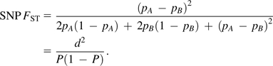This is a classical definition for SNP F_ST, where P is the MAF of the two populations combined, and d is the difference between the MAF of a population and P:

Hence, SNP F_ST is just a special case of microsatellite F_ST.

Unbiased Sample Statistic for F_ST

We compute unbiased sample statistics (which we refer to using a “hat” notation) separately for the numerator and denominator, then calculated the ratio.

Given sample sizes and unbiased sample statistics for mean and variance, the numerator becomes:

Similarly, the denominator becomes

Multiple Loci

All discussion so far has been for a single microsatellite locus. For K loci, we first compute K unbiased sample statistics, each for the numerator and denominator. Then we separately average the numerator and denominator and finally compute the ratio. This strategy avoids numerical instability issues of averaging ratios (namely, when denominators are small at certain loci).

Standard error across loci is computed via the jackknife method (Efron and Gong 1983). SNP F_ST quantities and standard errors were computed using EIGENSOFT (Patterson, Price, and Reich 2006).

Relating F_ST and ASD in Microsatellites

F_ST and ASD are closely related. From the above, it is clear that F_ST is a function of first- and second-order moments of allelic distributions. Furthermore, it is known (Goldstein et al. 1995a) that the ASD estimator is

Define X as the sum of intrapopulation variances. Define Y as interpopulation variance.

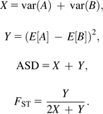Now the relationship between F_ST and ASD is clear. ASD closely resembles the total variance of allelic distributions of populations A and B combined. F_ST is the ratio of interpopulation variance to total variance.

Results

Microsatellite ASD and Sequence Divergence Are Linearly Related

To test empirically whether the microsatellite ASD statistic (Goldstein et al. 1995a) can be an unbiased estimate of t_MRCA, we used genomic sequence divergence as a “gold standard,” and assessed how closely the microsatellite inferences matched this number. We restricted our analysis to pairs of populations for which we had both extensive genome sequence alignments and large-scale microsatellite data. We first used sequence data sets to compute autosomal sequence divergence, which was assumed to be proportional to the average t_MRCA. This formed our gold-standard molecular clock. For the same pairs of populations, we then computed ASD using microsatellite data. Comparing sequence divergence to ASD provided a metric for the accuracy of the microsatellite molecular clock, assessed in terms of linearity (correlation coefficient) and standard errors.

FIgure 1 plots sequence divergence against microsatellite ASD. For WGS humans (Panel A), the correlation coefficient is r = 0.989 (P = 4.9e−7, 95% confidence interval [CI] 0.946–0.998). For RRS humans (Panel B), r = 0.983 (P = 5.3e−11, 95% CI 0.949–0.995). For chimpanzees (Panel C), r = 0.986 (P = 2.7e−4, 95% CI 0.877–0.999). Figure 1 suggests the following:

• Sequence divergence and microsatellite ASD are linearly related: The regressions have correlation coefficients all greater than 0.97. Because sequence divergence is known to be proportional to t_MRCA, microsatellite ASD is linear to t_MRCA. Interestingly, however, the regression lines do not intersect the origin, a point we return to below.

• Combining microsatellite loci yields a reasonably precise molecular clock and in principle supports precise inferences about history. Examining the standard errors in figure 1A, the 783 human microsatellite loci are approximately 2.5 times less precise than that of Biaka Pygmy sequence alignments. Thus, 783 microsatellite loci correspond to about 7.2 Mb of alignment of two WGS sequences (table 1). In turn, one microsatellite is “worth” approximately 10 kb of shotgun sequencing, which is expected to contain 10-nt mutations between two modern humans.

• The microsatellite molecular clock appears to be linear for at least 2 My: It has been shown theoretically that in the presence of severe range constraints, microsatellite ASD should lose its linear behavior after about 10,000 generations (Feldman et al. 1997), which is 250,000 years assuming 25 years per generation. Bonobos are a distinct species from chimpanzees, and are thought to have t_MRCA of around 2.2 My (Caswell et al. 2008) averaged across the genome, yet the linearity in figure 1C still applies to bonobo–chimpanzee divergence. Therefore, encouragingly, the duration of ASD linearity is at least 10 times that of theoretical predictions, suggesting range constraints are not as severe as previously imagined.

FIG. 1.—

Microsatellite ASD is linear with sequence divergence. Horizontal axes are sequence divergences measured in substitutions per kb, which we assume is an accurate gold standard. Vertical axes are microsatellite ASD values. Crosshairs are data with standard errors for each population pair. The linear regression line is shown. For WGS humans (A), the correlation coefficient is r = 0.989 (P = 4.9e−7, 95% CI 0.946–0.998). In the left box are Yoruba versus (top to bottom): European, East Asian, and Yoruba. In the right box are Biaka Pygmy versus (top to bottom): European, Yoruba, and East Asian. For RRS humans (B), r = 0.983 (P = 5.3e−11, 95% CI 0.949–0.995). In the left box are Yoruba versus (top to bottom): European, Australian Aborigine, East Asian, and Yoruba. In the right box is Biaka Pygmy versus: European, Yoruba, and East Asian; also are San versus: Yoruba, European, and East Asian. For chimpanzees (C), r = 0.986 (P = 2.7e−4, 95% CI 0.877–0.999).

Nonzero y-Intercept in figure 1

Although these results demonstrate microsatellites’ usefulness in estimating t_MRCA, there is a nonzero y-intercept (supplementary fig. S1, Supplementary Material online), oddly suggesting that zero sequence divergence (t_MRCA = 0) is associated with a positive ASD. We used simulations to investigate the possibility that microsatellite genotyping error caused the elevated ASD relative to its true value. Assuming a typical genotype error rate of 1% with error being randomly distributed at ±1 repeat length (Weber and Broman 2001), we can only explain 10% of the offset. It is possible, however, that the most pertinent error in microsatellite genotyping is not miscalling microsatellite lengths by a single repeat length, but instead, miscalling heterozygous genotypes as homozygous, which can easily occur with microsatellites (Weber and Broman 2001). Missing of heterozygotes would have the effect of generating false multi-step mutations, which would result in a much larger inflation in the ASD (due to the squaring of the difference in allele lengths) and could plausibly explain our significantly nonzero y-intercept. Alternatively, the relationship between ASD and t_MRCA could be globally nonlinear but easily linearizable in our time window. Whatever the cause for our observations, these results indicate that for population genetic analysis, it is important to use a calibration curve (such as fig. 1) to convert ASD to sequence divergence, correcting for the inflated estimate of divergence time from microsatellite ASD.

The Microsatellite Clock Reveals Deep Lineages of Human Genetic Variation

The microsatellite data show that the San, Biaka Pygmy, and Mbuti Pygmy Africans are more diverged in their pairwise t_MRCA from non-African populations than are Yoruba West Africans. These results are consistent with an analysis of microsatellite data by Zhivotovsky et al. (2003) but strengthen their result because microsatellite and sequence divergence concur (fig. 1A and B). It was already known based on mitochondrial DNA and Y chromosome data that the San and Mbuti contain deeply diverged lineages, but our results and those of Zhivotovsky et al. using autosomal microsatellite data show definitively that these populations are outgroups to all other populations.

Inferred Pairwise Sequence Divergence of HGDP Populations

An immediate application of the regressions from figure 1 is to infer sequence divergences for the remaining HGDP populations in which we lack sequence data. Figure 2 is a matrix plot showing the inferred divergences (hence inferred t_MRCA). In this plot, the San and Pygmy Africans are the only populations equidistant to all other populations, further suggesting that these populations are the most deeply diverged.

FIG. 2.—

Inferred pairwise sequence divergences of HGDP populations. Microsatellite ASD for each pair of populations in HGDP is computed. Then using regression from figure 1A, we inferred the divergence of each population pair in substitutions per kb. The grayscale intensities display the range of divergences. As shown, San and Pygmy Africans are equidistant from all other populations, suggesting that they have the largest t_MRCA to any other human population.

Microsatellite F_ST Accurately Estimates Allele Frequency Differentiation

F_ST measures the degree of differentiation between populations. Given genetic diversity data for two populations, F_ST (a quantity between 0 and 1) is the ratio of interpopulation variance to total variance. When F_ST is appropriately transformed (Slatkin 1991; Patterson unpublished), one can infer the genetic drift that occurred between two populations since they split. In particular, one can estimate the population split time (t_pop) in units of 2N, where N is the effective population size, under the assumption that populations have been constant in size since their divergence. We note that in human populations, t_pop and t_MRCA are different by an order of magnitude: For Africans versus non-Africans, the average t_MRCA is thought to be ∼500,000 years ago, whereas t_pop is thought to be 40,000–80,000 years ago (Keinan et al. 2008). As we have shown that the microsatellite molecular clock works for time depths of at least 2 My, we can be confident that it also works for time separations that are an order of magnitude less.

F_ST is usually estimated based on SNP and sequencing data when available, because uncertainties of the complex microsatellite mutation process confound the interpretation of a microsatellite F_ST in terms of history. Assuming the GSMM of microsatellite evolution, however, Slatkin derived a microsatellite-based F_ST estimator (Slatkin called it R_ST) (Slatkin 1995) that should be identical to SNP-based F_ST. The empirical analyses using Slatkin's estimator have been encouraging. For example, based on <300 SNPs (Fischer et al. 2006) and <300 microsatellites in four chimpanzee populations, Becquet et al. (2007) showed that the SNP F_ST and microsatellite F_ST were concordant.

As of today, the richest data sets with both genomewide SNPs and large numbers of microsatellites are those from HGDP (Rosenberg et al. 2002; Li et al. 2008). We computed and compared F_ST based on SNPs and microsatellites in these samples. An important distinction between the comparison we present here and that of the previous section (where we examined ASD) is that we do not assume SNP-based F_ST as gold standard.

Empirical Relationship between Microsatellite and SNP F_ST

Figure 3A plots SNP F_ST on the horizontal axis and microsatellite F_ST on the vertical axis. There are 53 populations in HGDP and hence 1,378 data points (53 choose 2) with standard errors. The linearity is clear and the regression lines intersect the origin. However, there are two distinct lines for F_ST > 0.1. The 1,035 pairwise comparisons of non-Africans populations (46 choose 2) have a regression line slope of 0.91 and correlation coefficient r = 0.983 (95% CI 0.982–0.986). The African versus non-African comparisons have a distinctly smaller slope of 0.73 and r = 0.969 (95% CI 0.962–0.975). It is evident that for F_ST > 0.1, SNP-based quantities are larger than microsatellite quantities when Africans are involved. We next investigate the possible reasons for this discrepancy.

FIG. 3.—

Microsatellite and SNP F_ST are almost equivalent, with the discrepancy likely due to SNP ascertainment. Horizontal axes are the SNP F_ST. Vertical axes are the microsatellite F_ST. In Panel A are F_ST computed from real HGDP data. There are (53 choose 2) = 1,378 pairwise population comparisons (data points). Circles and plus signs are data for each population pair. The linearity is clear, and the regression lines (not shown) intersect the origin. However, there are two distinct slopes for F_ST > 0.1. In circles are 1,035 (46 non-African populations, choose 2) non-Africans versus non-Africans, with regression line slope = 0.91 and correlation coefficient 0.983 (P < 1e−10, 95% CI 0.982–0.986). In plus signs are Africans versus all populations, with regression line slope = 0.73 and correlation coefficient 0.969 (P < 1e−10, 95% CI 0.962–0.975). In Panel B are simulated data (demographic model in supplementary fig. S2A, Supplementary Material online) with different SNP ascertainment schemes: No ascertainment in circles, ascertaining using two samples from population A (“African”) in dots, ascertaining using two samples from population B (“European”) in crosses, and ascertaining using one sample from each population in plus signs. In Panel C are simulated data (demographic model in supplementary fig. S2B, Supplementary Material online) of four populations resembling Africans, Europeans, East Asians, and Native Americans. We used the European-African ascertainment scheme (see text). In circles are non-Africans versus non-Africans. In plus signs are Africans versus non-Africans. For panels B and C, enough loci were simulated such that standard errors are of negligible magnitude.

SNP Ascertainment Bias Can Explain the Discrepancy between the Two F_ST Measurements

To investigate whether SNP ascertainment bias can explain the phenomena in figure 3A, we simulated SNP ascertainment as follows:

1. Demographic model 1 (supplementary fig. S2A, Supplementary Material online): The goal of this model is to generate a wide range of F_ST values, larger than that of real human populations. As shown in supplementary figure S2A, Supplementary Material online, the size of population A is fixed at N₀=10,000. The size of population B varies from 0.01N₀ to N₀, enabling an F_ST(A,B) range of 0.01–0.45. t_AB, the population separation time, is fixed at 400 generations.

2. Coalescent simulation and mutation generation: Given demographic model 1, we used Hudson's ms coalescent simulator (Hudson 2002) to generate trees and mutations assuming the infinite-sites model. Microsatellite alleles were then generated according to the SMM. Thus, each mutation is added or subtracted, at random, to the microsatellite lengths.

3. Ascertaining SNPs: To generate ascertainment bias-free SNPs, we recorded the derived allele frequency of each population across all loci. To generate SNPs affected by ascertainment bias, for each locus, we took two samples and examined the allele. If and only if they are different, we recorded the data from the locus, excluding the two used for ascertaining. We ascertain in three ways: 1) two samples from population A, 2) two samples from population B, and 3) one sample from each population.

4. F_ST calculation: With the data sets generated from simulated microsatellites and SNPs, we calculated F_ST. We examined if any of the three ascertainment schemes could generate the same directionality of bias as such in figure 3A.

5. Enhanced demographic model (supplementary fig. S2B, Supplementary Material online): The goals of this model are to more closely mimic real human history, and to apply the appropriate ascertainment scheme to all populations simultaneously and observe if ascertainment can cause the bias in figure 3A. As shown in supplementary figure S2B, Supplementary Material online, populations A, B, C, D are approximately Africans, Europeans, East Asians, and Native Americans, respectively. We used the same ascertainment scheme as above and estimated F_ST.

Simulations Can Replicate the Effect of Ascertainment Bias on SNPs

For demographic model 1, we denoted population A (the one with the larger effective population size) as “Africans” and population B as “non-Africans.” The simulation results are shown in figure 3B. Without ascertainment, both F_ST are identical. Ascertainment using two Africans showed negligible bias. Ascertainment using two non-Africans negatively biased SNP F_ST. Ascertainment using one sample from each population positively biased SNP F_ST. Compared with the real HGDP data (fig. 3A), ascertaining from one African and one non-African generated the same directional effect. This result is reasonable, because SNPs on medical genetics arrays were discovered as differences between a non-African chromosome and the reference human genome. The reference human genome sequence has a substantial amount of African ancestry because RPCI-11, the Bacterial Artificial Chromosome library that has contributed ∼74% of the human genome reference sequence (International Human Genome Sequencing Consortium 2001), is likely to be derived from an African American (Reich et al. 2009).

We applied the one African one non-African ascertainment scheme to demographic model 2. There are four populations in the model, producing six F_ST values in total (four choose two). As shown in figure 3C, the non-African versus non-African comparisons show little bias. The African versus non-African comparisons show a positively biased SNP F_ST. Thus, we have demonstrated that SNP ascertainment bias can generate the discrepancy in figure 3A.

A Unifying View of ASD and Microsatellite F_ST

Having established the accuracy of both microsatellite ASD and F_ST, we next show a 2D view of HGDP microsatellite data that highlights important historical events.

Just as sequence variation data contains information on both divergence time and genetic drift, it can be shown (Materials and Methods) that microsatellite ASD and F_ST are functions of two independent quantities: interpopulation variance and intrapopulation variance. Using the HGDP microsatellite data as previously described, in figure 4 we projected the data onto the two orthogonal statistics: interpopulation variance (horizontal axis) and intrapopulation variance (vertical axis). Again we have 1,378 data points, and lines of constant ASD and F_ST are marked. Above the thick black line are Africans versus all populations, and below are non-Africans versus non-Africans. This figure suggests the following:

• With the exception of Native American to Native American comparisons, lines of constant ASD have slopes similar to slopes of the data points. African populations are equidistant from non-Africans. This is expected from the “out-of-Africa” migration hypothesis in which all non-African populations form a clade (Cavalli-Sforza and Feldman 2003).

• Projecting onto lines of constant ASD, we see a clear gap (thick black line) between Africans and non-Africans. This confirms that there is a time difference between the out-of-Africa event and the rest of migration events. There is a second gap for the Native Americans, confirming that migration into America is a significantly more recent event (Cavalli-Sforza and Feldman 2003).

• Examining Africans versus all populations, F_ST projections show the drift out of Africa: The top left rectangle shows Africans versus Africans, followed by Europeans and Asians, then Pacific Islanders, and finally Native Americans (the rectangle crossing the largest F_ST values). The series of events is in agreement with progressive bottleneck events leading out of Africa (Ramachandran et al. 2005).

FIG. 4.—

A unifying view of ASD and microsatellite F_ST. The horizontal axis is interpopulation variance. The vertical axis is intrapopulation variance. Afr = Africans, NA = Native Americans, PI = Pacific Islanders, EA = East Asians, EMC = Europeans, Middle Easterners, and Central South Asians. It is shown (Materials and Methods) that microsatellite F_ST and ASD are functions of these two variances. Lines of constant ASD are dashed lines with negative slope. Lines of constant F_ST are dashed lines with positive slope. The data are (53 choose 2) = 1,378 pairwise HGDP population comparisons. Clearly, this picture segregates populations into distinguishable clusters. Africans versus all are above the thick black line. Non-Africans versus non-Africans are below the line. Distinguishable clusters are demarcated in ovals and squares.

Discussion

The fact that microsatellites are useful as molecular clocks has immediate applications: First, as described above (and in supplementary fig. S3, Supplementary Material online), we were able to use the clocklike nature of microsatellites to provide clear evidence that the San, Biaka, and Mbuti Pygmy branch off near the root of the tree of human populations, with all other populations (including West Africans) forming a clade. Note that all of our analyses are restricted to population average coalescent time, a quantity distinctly different and much more ancient than population split time. Second, we can use microsatellite data to correct inferences about F_ST based on high density SNP array data. SNP F_ST values can be precise, but they are affected by ascertainment bias. Potentially, we can use microsatellite F_ST to correct most of this bias. For example, based on figure 3, we estimate that all pairwise autosomal F_ST's between African and non-African populations in the Li et al. HGDP data (Li et al. 2008) are too large by a factor of 1.25 for F_ST values >0.1. By deflating all these F_ST values by this factor, we can obtain a pairwise F_ST matrix that is likely to be more accurate.

We finally note that our results are intriguing because in principle, they offer a way to obtain a direct estimate of the human per nucleotide mutation rate for sequence divergence data. To date, it has been impossible to obtain a direct estimate of the human per base pair mutation rate because the rate is too low (about 2 × 10⁻⁸ per nucleotide per generation) to permit direct observation from pedigree data. However, the microsatellite mutation rate is sufficiently high (10⁻³ to 10⁻⁴ per generation) that novel mutations are frequently directly observed in families (Weber and Wong 1993). By directly estimating the microsatellite mutation rate and mutation process in families, and then extrapolating to sequence divergence, we should be able to estimate the human per base pair mutation rate and infer the dates of important historical events, like the divergence times of human and chimpanzees, without using fossil records for calibration.

Supplementary Material

Supplementary figures S1–S3 and table S1 are available at Molecular Biology and Evolution online (http://www.mbe.oxfordjournals.org/).

References

- Altshuler D, Pollara VJ, Cowles CR, Van Etten WJ, Baldwin J, Linton L, Lander ES. An SNP map of the human genome generated by reduced representation shotgun sequencing. Nature. 2000;407:513–516. doi: 10.1038/35035083. [DOI] [PubMed] [Google Scholar]
- Amos W, Rubinstzein DC. Microsatellites are subject to directional evolution. Nat Genet. 1996;12:13–14. doi: 10.1038/ng0196-13. [DOI] [PubMed] [Google Scholar]
- Becquet C, Patterson N, Stone AC, Przeworski M, Reich D. Genetic structure of chimpanzee populations. PLoS Genet. 2007;3:e66. doi: 10.1371/journal.pgen.0030066. [DOI] [PMC free article] [PubMed] [Google Scholar]
- Bowcock AM, Ruiz-Linares A, Tomfohrde J, Minch E, Kidd JR, Cavalli-Sforza LL. High resolution of human evolutionary trees with polymorphic microsatellites. Nature. 1994;368:455–457. doi: 10.1038/368455a0. [DOI] [PubMed] [Google Scholar]
- Caswell JL, Mallick S, Richter DJ, Neubauer J, Schirmer C, Gnerre S, Reich D. Analysis of chimpanzee history based on genome sequence alignments. PLoS Genet. 2008;4:e1000057. doi: 10.1371/journal.pgen.1000057. [DOI] [PMC free article] [PubMed] [Google Scholar]
- Cavalli-Sforza LL, Feldman MW. The application of molecular genetic approaches to the study of human evolution. Nat Genet. 2003;33(Suppl):266–275. doi: 10.1038/ng1113. [DOI] [PubMed] [Google Scholar]
- Chimpanzee Sequencing and Analysis Consortium. Initial sequence of the chimpanzee genome and comparison with the human genome. Nature. 2005;437:69–87. doi: 10.1038/nature04072. [DOI] [PubMed] [Google Scholar]
- Clark AG, Hubisz MJ, Bustamante CD, Williamson SH, Nielsen R. Ascertainment bias in studies of human genome-wide polymorphism. Genome Res. 2005;15:1496–1502. doi: 10.1101/gr.4107905. [DOI] [PMC free article] [PubMed] [Google Scholar]
- Conrad DF, Jakobsson M, Coop G, Wen X, Wall JD, Rosenberg NA, Pritchard JK. A worldwide survey of haplotype variation and linkage disequilibrium in the human genome. Nat Genet. 2006;38:1251–1260. doi: 10.1038/ng1911. [DOI] [PubMed] [Google Scholar]
- Di Rienzo A, Peterson AC, Garza JC, Valdes AM, Slatkin M, Freimer NB. Mutational processes of simple-sequence repeat loci in human populations. Proc Natl Acad Sci USA. 1994;91:3166–3170. doi: 10.1073/pnas.91.8.3166. [DOI] [PMC free article] [PubMed] [Google Scholar]
- Dib C, Faure S, Fizames C, et al. (13 co-authors) A comprehensive genetic map of the human genome based on 5,264 microsatellites. Nature. 1996;380:152–154. doi: 10.1038/380152a0. [DOI] [PubMed] [Google Scholar]
- Efron B, Gong G. A leisurely look at the bootstrap, the jackknife, and cross-validation. Am Stat. 1983;37:36–48. [Google Scholar]
- Ellegren H. Microsatellite mutations in the germline: implications for evolutionary inference. Trends Genet. 2000;16:551–558. doi: 10.1016/s0168-9525(00)02139-9. [DOI] [PubMed] [Google Scholar]
- Ellegren H. Microsatellites: simple sequences with complex evolution. Nat Rev Genet. 2004;5:435–445. doi: 10.1038/nrg1348. [DOI] [PubMed] [Google Scholar]
- Feldman MW, Bergman A, Pollock DD, Goldstein DB. Microsatellite genetic distances with range constraints: analytic description and problems of estimation. Genetics. 1997;145:207–216. doi: 10.1093/genetics/145.1.207. [DOI] [PMC free article] [PubMed] [Google Scholar]
- Fischer A, Pollack J, Thalmann O, Nickel B, Paabo S. Demographic history and genetic differentiation in apes. Curr Biol. 2006;16:1133–1138. doi: 10.1016/j.cub.2006.04.033. [DOI] [PubMed] [Google Scholar]
- Friedlaender JS, Friedlaender FR, Reed FA, et al. (11 co-authors) The genetic structure of Pacific Islanders. PLoS Genet. 2008;4:e19. doi: 10.1371/journal.pgen.0040019. [DOI] [PMC free article] [PubMed] [Google Scholar]
- Goldstein DB, Pollock DD. Launching microsatellites: a review of mutation processes and methods of phylogenetic interference. J Hered. 1997;88:335–342. doi: 10.1093/oxfordjournals.jhered.a023114. [DOI] [PubMed] [Google Scholar]
- Goldstein DB, Ruiz Linares A, Cavalli-Sforza LL, Feldman MW. An evaluation of genetic distances for use with microsatellite loci. Genetics. 1995a;139:463–471. doi: 10.1093/genetics/139.1.463. [DOI] [PMC free article] [PubMed] [Google Scholar]
- Goldstein DB, Ruiz Linares A, Cavalli-Sforza LL, Feldman MW. Genetic absolute dating based on microsatellites and the origin of modern humans. Proc Natl Acad Sci USA. 1995b;92:6723–6727. doi: 10.1073/pnas.92.15.6723. [DOI] [PMC free article] [PubMed] [Google Scholar]
- Hudson RR. Generating samples under a Wright–Fisher neutral model of genetic variation. Bioinformatics. 2002;18:337–338. doi: 10.1093/bioinformatics/18.2.337. [DOI] [PubMed] [Google Scholar]
- International Human Genome Sequencing Consortium. Initial sequencing and analysis of the human genome. Nature. 2001;409:860–921. doi: 10.1038/35057062. [DOI] [PubMed] [Google Scholar]
- Keinan A, Mullikin JC, Patterson N, Reich D. Accelerated genetic drift on chromosome X during the human dispersal out of Africa. Nat Genet. 2008;41:66–70. doi: 10.1038/ng.303. [DOI] [PMC free article] [PubMed] [Google Scholar]
- Keinan A, Mullikin JC, Patterson N, Reich D. Measurement of the human allele frequency spectrum demonstrates greater genetic drift in East Asians than in Europeans. Nat Genet. 2007;39:1251–1255. doi: 10.1038/ng2116. [DOI] [PMC free article] [PubMed] [Google Scholar]
- Kimmel M, Chakraborty R. Measures of variation at DNA repeat loci under a general stepwise mutation model. Theor Popul Biol. 1996;50:345–367. doi: 10.1006/tpbi.1996.0035. [DOI] [PubMed] [Google Scholar]
- Kimmel M, Chakraborty R, King JP, Bamshad M, Watkins WS, Jorde LB. Signatures of population expansion in microsatellite repeat data. Genetics. 1998;148:1921–1930. doi: 10.1093/genetics/148.4.1921. [DOI] [PMC free article] [PubMed] [Google Scholar]
- Kruglyak S, Durrett RT, Schug MD, Aquadro CF. Equilibrium distributions of microsatellite repeat length resulting from a balance between slippage events and point mutations. Proc Natl Acad Sci USA. 1998;95:10774–10778. doi: 10.1073/pnas.95.18.10774. [DOI] [PMC free article] [PubMed] [Google Scholar]
- Levinson G, Gutman GA. High frequencies of short frameshifts in poly-CA/TG tandem repeats borne by bacteriophage M13 in Escherichia coli K-12. Nucleic Acids Res. 1987;15:5323–5338. doi: 10.1093/nar/15.13.5323. [DOI] [PMC free article] [PubMed] [Google Scholar]
- Li JZ, Absher DM, Tang H, et al. (10 co-authors) Worldwide human relationships inferred from genome-wide patterns of variation. Science. 2008;319:1100–1104. doi: 10.1126/science.1153717. [DOI] [PubMed] [Google Scholar]
- Nauta MJ, Weissing FJ. Constraints on allele size at microsatellite loci: implications for genetic differentiation. Genetics. 1996;143:1021–1032. doi: 10.1093/genetics/143.2.1021. [DOI] [PMC free article] [PubMed] [Google Scholar]
- Ning Z, Cox AJ, Mullikin JC. SSAHA: a fast search method for large DNA databases. Genome Res. 2001;11:1725–1729. doi: 10.1101/gr.194201. [DOI] [PMC free article] [PubMed] [Google Scholar]
- Ohta T, Kimura M. A model of mutation appropriate to estimate the number of electrophoretically detectable alleles in a finite population. Genet Res. 1973;22:201–204. doi: 10.1017/s0016672300012994. [DOI] [PubMed] [Google Scholar]
- Paetkau D, Waits LP, Clarkson PL, Craighead L, Strobeck C. An empirical evaluation of genetic distance statistics using microsatellite data from bear (Ursidae) populations. Genetics. 1997;147:1943–1957. doi: 10.1093/genetics/147.4.1943. [DOI] [PMC free article] [PubMed] [Google Scholar]
- Patterson N, Price AL, Reich D. Population structure and eigenanalysis. PLoS Genet. 2006;2:e190. doi: 10.1371/journal.pgen.0020190. [DOI] [PMC free article] [PubMed] [Google Scholar]
- Patterson N, Richter DJ, Gnerre S, Lander ES, Reich D. Genetic evidence for complex speciation of humans and chimpanzees. Nature. 2006;441:1103–1108. doi: 10.1038/nature04789. [DOI] [PubMed] [Google Scholar]
- Ramachandran S, Deshpande O, Roseman CC, Rosenberg NA, Feldman MW, Cavalli-Sforza LL. Support from the relationship of genetic and geographic distance in human populations for a serial founder effect originating in Africa. Proc Natl Acad Sci USA. 2005;102:15942–15947. doi: 10.1073/pnas.0507611102. [DOI] [PMC free article] [PubMed] [Google Scholar]
- Ramachandran S, Rosenberg NA, Feldman MW, Wakeley J. Population differentiation and migration: coalescence times in a two-sex island model for autosomal and X-linked loci. Theor Popul Biol. 2008;74:291–301. doi: 10.1016/j.tpb.2008.08.003. [DOI] [PMC free article] [PubMed] [Google Scholar]
- Reich DE, Goldstein DB. Genetic evidence for a Paleolithic human population expansion in Africa. Proc Natl Acad Sci USA. 1998;95:8119–8123. doi: 10.1073/pnas.95.14.8119. [DOI] [PMC free article] [PubMed] [Google Scholar]
- Reich D, Nalls MA, Kao WHL, et al. (20 co-authors) Reduced neutrophil count in people of African descent is due to a regulatory variant in the Duffy Antigen Receptor for Chemokines gene. PLoS Genetics. 2009;5:e1000360. doi: 10.1371/journal.pgen.1000360. [DOI] [PMC free article] [PubMed] [Google Scholar]
- Roder MS, Korzun V, Wendehake K, Plaschke J, Tixier MH, Leroy P, Ganal MW. A microsatellite map of wheat. Genetics. 1998;149:2007–2023. doi: 10.1093/genetics/149.4.2007. [DOI] [PMC free article] [PubMed] [Google Scholar]
- Rosenberg NA. The probability of topological concordance of gene trees and species trees. Theor Popul Biol. 2002;61:225–247. doi: 10.1006/tpbi.2001.1568. [DOI] [PubMed] [Google Scholar]
- Rosenberg NA. Standardized subsets of the HGDP–CEPH Human Genome Diversity Cell Line Panel, accounting for atypical and duplicated samples and pairs of close relatives. Ann Hum Genet. 2006;70:841–847. doi: 10.1111/j.1469-1809.2006.00285.x. [DOI] [PubMed] [Google Scholar]
- Rosenberg NA, Mahajan S, Gonzalez-Quevedo C, et al. (12 co-authors) Low levels of genetic divergence across geographically and linguistically diverse populations from India. PLoS Genet. 2006;2:e215. doi: 10.1371/journal.pgen.0020215. [DOI] [PMC free article] [PubMed] [Google Scholar]
- Rosenberg NA, Mahajan S, Ramachandran S, Zhao C, Pritchard JK, Feldman MW. Clines, clusters, and the effect of study design on the inference of human population structure. PLoS Genet. 2005;1:e70. doi: 10.1371/journal.pgen.0010070. [DOI] [PMC free article] [PubMed] [Google Scholar]
- Rosenberg NA, Pritchard JK, Weber JL, Cann HM, Kidd KK, Zhivotovsky LA, Feldman MW. Genetic structure of human populations. Science. 2002;298:2381–2385. doi: 10.1126/science.1078311. [DOI] [PubMed] [Google Scholar]
- Sainudiin R, Durrett RT, Aquadro CF, Nielsen R. Microsatellite mutation models: insights from a comparison of humans and chimpanzees. Genetics. 2004;168:383–395. doi: 10.1534/genetics.103.022665. [DOI] [PMC free article] [PubMed] [Google Scholar]
- Shimoda N, Knapik EW, Ziniti J, Sim C, Yamada E, Kaplan S, Jackson D, de Sauvage F, Jacob H, Fishman MC. Zebrafish genetic map with 2000 microsatellite markers. Genomics. 1999;58:219–232. doi: 10.1006/geno.1999.5824. [DOI] [PubMed] [Google Scholar]
- Slatkin M. A measure of population subdivision based on microsatellite allele frequencies. Genetics. 1995;139:457–462. doi: 10.1093/genetics/139.1.457. [DOI] [PMC free article] [PubMed] [Google Scholar]
- Slatkin M. Inbreeding coefficients and coalescence times. Genet Res. 1991;58:167–175. doi: 10.1017/s0016672300029827. [DOI] [PubMed] [Google Scholar]
- Szpiech ZA, Jakobsson M, Rosenberg NA. ADZE: a rarefaction approach for counting alleles private to combinations of populations. Bioinformatics. 2008;24:2498–2504. doi: 10.1093/bioinformatics/btn478. [DOI] [PMC free article] [PubMed] [Google Scholar]
- Valdes AM, Slatkin M, Freimer NB. Allele frequencies at microsatellite loci: the stepwise mutation model revisited. Genetics. 1993;133:737–749. doi: 10.1093/genetics/133.3.737. [DOI] [PMC free article] [PubMed] [Google Scholar]
- Wang S, Lewis CM, Jakobsson M, et al. (26 co-authors) Genetic variation and population structure in native Americans. PLoS Genet. 2007;3:e185. doi: 10.1371/journal.pgen.0030185. [DOI] [PMC free article] [PubMed] [Google Scholar]
- Wang S, Ray N, Rojas W, et al. (27 co-authors) Geographic patterns of genome admixture in Latin American Mestizos. PLoS Genet. 2008;4:e1000037. doi: 10.1371/journal.pgen.1000037. [DOI] [PMC free article] [PubMed] [Google Scholar]
- Weber JL, Broman KW. Genotyping for human whole-genome scans: past, present, and future. Adv Genet. 2001;42:77–96. doi: 10.1016/s0065-2660(01)42016-5. [DOI] [PubMed] [Google Scholar]
- Weber JL, Myers EW. Human whole-genome shotgun sequencing. Genome Res. 1997;7:401–409. doi: 10.1101/gr.7.5.401. [DOI] [PubMed] [Google Scholar]
- Weber JL, Wong C. Mutation of human short tandem repeats. Hum Mol Genet. 1993;2:1123–1128. doi: 10.1093/hmg/2.8.1123. [DOI] [PubMed] [Google Scholar]
- Xu X, Peng M, Fang Z. The direction of microsatellite mutations is dependent upon allele length. Nat Genet. 2000;24:396–399. doi: 10.1038/74238. [DOI] [PubMed] [Google Scholar]
- Zhivotovsky LA. Estimating divergence time with the use of microsatellite genetic distances: impacts of population growth and gene flow. Mol Biol Evol. 2001;18:700–709. doi: 10.1093/oxfordjournals.molbev.a003852. [DOI] [PubMed] [Google Scholar]
- Zhivotovsky LA, Rosenberg NA, Feldman MW. Features of evolution and expansion of modern humans, inferred from genomewide microsatellite markers. Am J Hum Genet. 2003;72:1171–1186. doi: 10.1086/375120. [DOI] [PMC free article] [PubMed] [Google Scholar]
- Zuckerkandl E, Pauling L. Molecular disease, evolution, and genetic heterogeneity. In: Kasha M, Pullman B, editors. Horizons in biochemistry. New York: Academic Press; 1962. pp. 189–225. [Google Scholar]
Associated Data
This section collects any data citations, data availability statements, or supplementary materials included in this article.