Inferring Population Mutation Rate and Sequencing Error Rate Using the SNP Frequency Spectrum in a Sample of DNA Sequences

Abstract

One challenge of analyzing samples of DNA sequences is to account for the nonnegligible polymorphisms produced by error when the sequencing error rate is high or the sample size is large. Specifically, those artificial sequence variations will bias the observed single nucleotide polymorphism (SNP) frequency spectrum, which in turn may further bias the estimators of the population mutation rate $\theta =4N\mu$ for diploids. In this paper, we propose a new approach based on the generalized least squares (GLS) method to estimate θ, given a SNP frequency spectrum in a random sample of DNA sequences from a population. With this approach, error rate ε can be either known or unknown. In the latter case, ε can be estimated given an estimation of θ. Using coalescent simulation, we compared our estimators with other estimators of θ. The results showed that the GLS estimators are more efficient than other θ estimators with error, and the estimation of ε is usable in practice when the θ per bp is small. We demonstrate the application of the estimators with 10-kb noncoding region sequence sampled from a human population and provide suggestions for choosing θ estimators with error.

1. Introduction

Sequencing errors can produce many problems for evolutionary or population genetical analysis of samples of DNA sequences (Clark and Whittam 1992, Johnson and Slatkin 2008). Given a random sample of sequence from a population, artificial polymorphisms caused by sequencing error will skew both the number and the frequency spectrum of the observed single nucleotide polymorphisms (SNPs). This will further skew any estimations or tests based on the number and/or frequency spectrum of the SNPs if errors are not properly taken into account. The bias will be more prominent with increased sample size because sequencing error accumulates linearly with sample size while θ increases slower, as implied by coalescent theory. Johnson and Slatkin (2008) suggested a rule of thumb that an uncorrected estimate will be biased significantly if $n\epsilon \ge \theta /L$, where n is the sample size (i.e., number of sequences), ε is the average error rate per site, L is the sequence length of the given locus, and θ is the population mutation rate of the locus. θ is equal to $4N\mu$ for diploids and $2N\mu$ for haploids, where N is the effective population size and μ is the mutation rate for the given locus. $\theta /L$ typically ranges from $10^{-4}$ for species with extremely low diversity, such as the bog turtle (Rosenbaum et al. 2007), to $10^{-2}$ for species with extremely high diversity, such as human immunodeficiency virus (Achaz et al. 2004). For human populations, $\theta /L$ is approximately $10^{-3}$ (Crawford et al. 2005). Therefore, with a typical sequencing error rate of $10^{-5}$ on the Sanger sequencing platform (Zwick 2005), uncorrected estimates will have problem with larger than 50 individuals (100 chromosomes) in human populations. If next-generation sequencing technologies are used, their higher sequencing error ($10^{-4}$) (Mackay et al. 2008, Shendure and Ji 2008) may further reduce the upper limit of sample size to only 10 chromosomes or less.

In response to the problem, researchers are developing new unbiased estimators and tests for population samples with sequencing error incorporated into the analysis. Johnson and Slatkin (2006) proposed maximum likelihood estimators for θ and the scaled exponential growth rate using the SNP frequency spectrum while accounting for sequencing error via Phred quality scores. They also studied the effects of sequencing error on two uncorrected estimators of θ, Tajima's (Tajima 1983) and Watterson's (Watterson 1975), and proposed two unbiased estimators of θ assuming known ε (see discussions below) (Johnson and Slatkin 2008). Hellmann et al. (2008) proposed a method to correct , assuming known ε. It is similar to Johnson and Slatkin (2008)‘s θ estimator based on the total number of polymorphic sites but takes account of the uncertainty of chromosome sampling in a shot-gun sequencing of mixed diploid individuals. Lynch (2008) proposed several methods to correct for high-coverage shot-gun genomic sequences from a single diploid individual. Knudsen and Miyamoto (2007) incorporated missing data, sequencing error, and multiple reads for diploid individuals into a full-likelihood coalescent model of a sample of DNA sequences. Their model can be used to estimate θ and ε jointly. However, the computational intensity of calculating the likelihood limits the application of the model to small sample sizes (i.e., less than 20 sequences). Assuming a low but unknown ε, Achaz (2008) proposed two new moment estimators of θ based on the SNP number and frequency spectrum while ignoring singletons, on which sequencing error skews the most, and constructed two new test statistics for neutrality based on the new estimators. Jiang et al. (2009) developed a method to estimate θ and recombination rate for shot-gun resequencing data and proposed some refinements to increase its robustness to sequencing errors.

Here, we propose a new approach based on the generalized least squares (GLS) method to estimate θ using the SNP frequency spectrum of a random sample of DNA sequences from a population. It can be considered as a modification and extension of Fu (1994b)‘s best linear unbiased estimator (BLUE) estimator under the assumption of a moderate to low ε, either known or unknown. When ε is unknown, it can be estimated sequentially after the estimation of θ. The rational here is to incorporate the variance–covariance structure of the SNP frequency spectrum, with either known or unknown ancestral states of the SNPs, and reduce the variation of the estimator. Its computational intensity is higher than Achaz (2008)‘s moment estimators but much lower than Knudsen and Miyamoto (2007)‘s full-likelihood method, which makes it applicable to samples with thousands of sequences. In the following sections, we first introduce our GLS estimators along with some corrected or uncorrected estimators of θ; then, we compare these estimators using coalescent simulation assuming different population parameters. We demonstrate their application on a sample of DNA sequences of a 10-kilobase noncoding region on human chromosome 22. Finally, we discuss the advantages, limitations, and some technical issues of the GLS estimators.

2. Methods

2.1. Assumptions

Sequencing error at each site is usually modeled as a binomial or Poisson variable with parameter $p=n\epsilon$. As defined in the Introduction, n is the sample size (i.e., number of sequences) and ε is the average error rate per site. Here, we simplify the model by assuming that each site has at most one sequencing error, which occurs with probability P. As a rule of thumb, this assumption is approximately valid with $P\hspace{0.17em}<\hspace{0.17em}0.01$. We further assume that when a sequencing error occurs on an ancestral (or mutant) allele, the probability that it leads to an existing allele (mutant or ancestral) is u and the probability that it yields a new allele is $1-u$. For example, if only point mutation is considered and assuming that a nucleotide has equal probability to be read incorrectly as one of the other three nucleotides, $u=1/3$. For a sample of n sequences with length L randomly sampled from a population, we designate ${\xi }_i$ as the (unknown) number of true polymorphic sites with mutation size i (or SNP class i, i.e., there are i copies of the mutant allele in the sample) and ${\xi }_{i,k}$ as the observed number of sites with $n-i-k$ copies of the ancestral allele, i copies of the mutant alleles and k copy of the new allele (other than mutant and ancestral alleles) produced by sequencing error ($k=0,1$).

2.2. Approximate GLS Estimators of θ When ε is Unknown

If ε or p is unknown but assumed to be relatively small, it is easy to see that most errors are singletons (${\xi }_{0,1}$ or ${\xi }_{n-1,1}$) because ${\xi }_0\gg {\sum }_{i=1}^{n-1}{\xi }_i$ with assumption of infinite site model and a reasonable θ (Achaz 2008). In another words, ${\xi }_i\approx {\xi }_{i,0}$ for $2\le i\le n-1$. By ignoring singletons, we removed most of the errors so that $\epsilon \approx 0$ in the remaining SNP classes based on which new estimators can be developed. For example, Achaz (2008) proposed _{K − ξ1} and _{K− η1} estimators, which are modified Watterson (1975)‘s estimator and _{π− ξ1} and _{π − η1} estimators, which are modified Tajima (1983)‘s estimator (see details below). Fu (1994b) proposed a θ estimator based on the GLS method (_BLUEu and _BLUEf, called BLUE estimators in Fu 1994b), which makes full use of the observed numbers of SNP frequency classes, so that it has much less variability than either Watterson (1975)‘s or Tajima (1983)‘s estimator.

Following Achaz (2008)‘s idea that because singletons are much more likely to be errors comparing to other SNP class, an estimator based on the SNP spectrum excluding singletons will be robust to errors. Here, we briefly describe the modification of Fu (1994b)‘s GLS method by ignoring all singletons and triple allele. See Fu (1994a, 1994b) for more technique details of the method. We first rewrite the expectations, variances, and covariances of the observed number of SNP classes as:

(1)

(2)

(3)

where $1\le i\le n-1$. The values of ρ_i and ${\sigma }_{ij}$ are dependent on the population model, which can be obtained theoretically or numerically using simulation. Assuming a Wright–Fisher model with constant population size, no selection, and recombination, their explicit formulas are known (Fu 1995). Writing in a matrix form, we have

where

and is calculated with equations (2) and (3). Then, the corresponding GLS estimator of θ is

Because the calculation of needs prior estimation of θ, the _BLUE−ξ1 is calculated iteratively (Fu 1994a, 1994b): 1) give an initial value of θ, say θ₀ = , 2) calculate with θ₀; 3) calculate _{BLUE − ξ1} with and let θ₁ =_{BLUE − ξ1}; 4) update with ${\theta }_1$; and 5) repeat step 3 and 4 until _{BLUE − ξ1} converges.

If the ancestral state of each SNP is unknown (i.e., we do not know which allele is ancestral and which is mutant) then we need to fold the counting of ξ_i and ${\xi }_{n-i}$ to include all SNPs with a minor allele frequency i and major allele frequency $n-i$ or vice versa. In the folded case,

and is changed accordingly. The corresponding estimator, designated as _{BLUE − η1}, can be calculated with the same iterative process as described above.

After the θ is estimated, p can be approximated as

(4)

for unfolded counting or

(5)

for folded counting, where E(ξ₁ |) and E(ξ_n−1|) are calculated using equation (1) with θ replaced by . Then, is simply /n. For convenience, we use the subscript of the θ estimator used in to designate different s. For example, _{BLUE − ξ1} means the calculated using _{BLUE− ξ1}.

2.3. GLS Estimators of θ When ε is Known

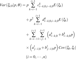
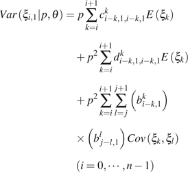
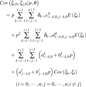
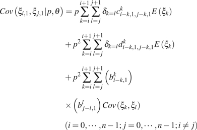
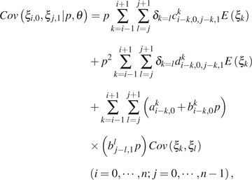
When ε is known, we can develop a more precise GLS estimator of θ by making full use of this information. First, we need to derive expectations, variance, and covariances of ${\xi }_{i,k}$. For simplicity, letting ${\xi }_i=0$ if $i\hspace{0.17em}<\hspace{0.17em}0$ or $i\ge n$ then

(6)

(7)

(8)

(9)

(10)

(11)

(12)

where ${\delta }_{k=l}$ is an index function, which equals to 1 if $k=l$ or 0 otherwise; a_m,jⁱ, b_m,jⁱ, c _m,j1,k,j2ⁱ, and d_m,j1,k,j2ⁱ are functions of i, j, $j_1$, $j_2$, m, k, n, and u. Their detailed expression and the derivation of the above formulas can be found in the Appendix. $E({\xi }_i)$, $Var({\xi }_i)$, and $Cov({\xi }_i,{\xi }_j)$$(1\le i,j\le n-1)$ can be calculated using equations (1)–(3).

In practice, ${\xi }_{1,0}$ and ${\xi }_{0,1}$ are indistinguishable even when the ancestral states are known. To avoid the above difficulties, we combine observations of ${\xi }_{1,0}$ and ${\xi }_{0,1}$. The general formulas for calculating the expectation of the combined observations and the variance–covariance of the combined observation with other (combined) observations are

(13)

(14)

(15)

(16)

where ${\xi }_{x_i,y_i}$, ${\xi }_{w,z}$, and ${\xi }_{w_j,z_j}$ can be any given ${\xi }_{k,0}$ or ${\xi }_{k,1}$. For example, to apply equations (13)–(14) to ${\xi }_{1,0}$ and ${\xi }_{0,1}$, we simply let $x_1=1$, $y_1=0$, $x_2=0$, and $y_2=1$. By incorporating $E({\xi }_0)=L-{\sum }_{i=1}^{n-1}E({\xi }_i)$, we have

A GLS estimator can be calculated as follows. If the ancestral state of each site is known or can be inferred from outgroups, let

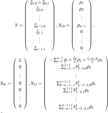then

(17)

The GLS estimator of θ is

(18)

again is an estimation of the variance–covariance matrix of Y , which can be calculated using equations (8)–(16). The same iterative process described above is then used to calculate _GLS. In the case that ancestral states are unknown, we need to further fold ${\xi }_{i,0}$ with ${\xi }_{n-i,0}$, and ${\xi }_{i,1}$ with ${\xi }_{n-i-1,1}$ because they are indistinguishable. Let

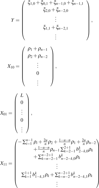and follow the same steps as described for _GLS. We can calculate the GLS estimator with folded observations. Later in this paper, we designate _GLSf to be the GLS estimator using folded observations and _GLSu to be that using unfolded observations.

2.4. Comparing to Other Estimators of θ Using Simulation

Three types of corrected and uncorrected estimators of θ were compared in this study, which will be briefly introduced below. Johnson and Slatkin (2006)‘s method was not compared because here, we assume the detailed Phred quality scores is unknown. Neither did we include Knudsen and Miyamoto (2007)‘s method because of its computational intensity and limitation to small sample sizes. Hellmann et al. (2008) and Johnson and Slatkin (2008)‘s estimators based on the total number polymorphic sites should have similar performances, so only the latter was included in our comparison.

The first type of estimator (type I) is based on the total number of polymorphic sites. An uncorrected estimator of this type is the widely used Watterson's estimator = K/a_n (Watterson 1975), where $a_n={\sum }_{i=1}^{n-1}1/i$ and K is the total number of polymorphic sites in the sample. Assuming a known ε, Johnson and Slatkin (2008) proposed a corrected estimator (with modification):

where

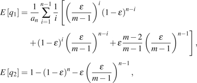and m is the total number of possible alleles in a site. Assuming an unknown but small ε, Achaz (2008) proposed two corrected estimators of this type. They are for unfolded observations and for folded observations.

The second type of estimator (type II) is based on the average difference between two sequences. An uncorrected estimator of this type is Tajima's (Tajima 1983), where ${\pi }_{ij}$ is the number of difference between sequences i and j. Johnson and Slatkin (2008)‘s corrected estimator of this type (with modification) is

where

Achaz (2008)‘s corrected estimators of this type are

for unfolded observations and

for folded observations.

The third type of estimator (type III) compared is the GLS estimator. Our estimators are corrected GLS estimators, which can be considered an extension to Fu (1994b)‘s uncorrected GLS estimators _BLUEu and _BLUEf for unfolded and folded counting, respectively.

We compared the performances of the estimators using coalescent simulations (e.g., Hudson 2002). We assumed a Wright–Fisher model with constant population size, no selection, no recombination and a simple infinite sites model for mutation. For each combination of parameters, 10,000 samples were simulated. Only point mutations ($u=1/3$) were simulated. The GLS estimation iteration was stopped either when the absolute value change between the update of _GLS is smaller than $10^{-3}$ or when 200 updates of equation (18) was conducted (see Methods for details). Sequencing error at each site was simulated to follow a binomial distribution with parameter p. Because _{BLUE − ξ1}, _{BLUE − η1}, , , , , _BLUEu, and _BLUEf assume at most two alleles at each site, for those estimators if a site has more than one type of non-ancestral allele, the one with the largest count is regarded as the mutant allele and all other non-ancestral alleles are regarded as errors from ancestral alleles. For example, if a site has two non-ancestral alleles with counts 1 and 2 then it will be added to ${\xi }_2$ instead of ${\xi }_1$. was calculated with equation (4) using _{BLUE −ξ1}, , and or with equation (5) using _{BLUE − η1}, , and .

3. RESULTS

3.1. Simulation Comparison

For each set of simulated samples with a given combination of parameters, we compared the mean and variance of each estimator. We also calculated the mean squared error (MSE) of each estimator and the variance of an optimal estimator, $V_{min}$. For θ, the large-sample approximation of $V_{min}$ is $V_{min}\left(\theta \right)=\theta [{\sum }_{i=1}^{n-1}(\theta +i{)}^{-1}{]}^{-1}$ (Fu and Li 1993). Because we know the actual number of errors introduced in each simulated sample, say $n_{err}$, we simply use $n_{err}/nL$ as the optimal estimator of ε and calculated its variance $V_{min}(\epsilon )$ in simulated samples. The ratio $V_{min}/MSE$ indicates the relative efficiency of each estimator to the optimal estimator.

As expected, with increasing p, via either an increasing error rate ε or an increasing sample size n, the uncorrected θ estimators perform poorly (data not shown). The four uncorrected θ estimators (, , _BLUEu, and _BLUEf) are upper biased significantly with increasing ε because they assume every polymorphism is a result of mutation. As a result, the uncorrected θ estimators are the least efficient estimators comparing to the corrected ones (data not shown). Among them, _BLUEu and _BLUEf are the most sensitive to sequencing error, whereas is the least sensitive. Looking at this in another way, although under the null hypothesis of no sequencing error, the order of their relative efficiency is , the order is totally reversed when p is larger. The above observations can be partially explained by the weight each estimator puts on ${\xi }_i$. Although puts equal weight on every ${\xi }_i$, puts less weight on ${\xi }_i$ than on ${\xi }_j$ if $i\hspace{0.17em}<\hspace{0.17em}j$. On the contrary, _BLUEu puts more weight on ${\xi }_i$ because under the assumption of no error, ${\xi }_i$ is a more reliable observation than ${\xi }_j$. However, the opposite is true with errors.

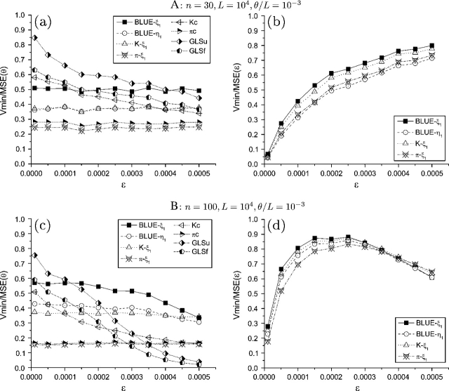
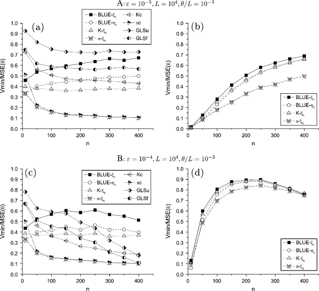
On the other hand, the efficiency of corrected θ estimators is less affected by increasing p. As to those with unknown ε, all are approximately unbiased. Their variances are relatively unchanged with the increase of ε or even decrease slightly with an increase of n (data not shown). The order of their efficiency is (figs. 1 and 2, and are not shown because they have a very similar efficiency as and , respectively). For the estimators with known ε, all of them are approximately unbiased except that _GLSu and _GLSf are upper biased when $p\hspace{0.17em}>\hspace{0.17em}0.01$. The variances of _kc, _GLSu and _GLSf increase with the increase of ε or n except when n is small (say < 100). As a result, their efficiency decreases with increasing p (figs. 1 and 2). With $p<0.01$, the order of their efficiency is (figs. 1 and 2). In summary, with a small to moderate ε (when $P\hspace{0.17em}<\hspace{0.17em}0.01$ and known), _GLSu and _GLSf are the most efficient θ estimators; otherwise, and are the most efficient estimators.

FIG. 1.—

Efficiency of θ and ε estimators with increase of ε. Only the subscripts of the estimators were shown.

FIG. 2.—

Efficiency of θ and ε estimators with increase of n. Only the subscripts of the estimators were shown.

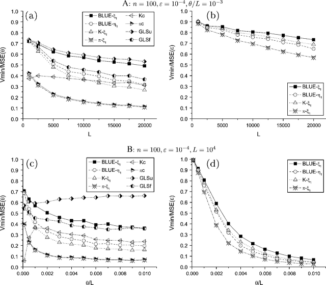
Increasing θ, either by increasing $\theta /L$ or by L, affects the variances but not the means of the θ estimators. The variances of all estimators increase with the increase of θ. As a result, the efficiency of corrected estimators decrease with an increase of θ, with the exception of _Kc, which actually increases when $\theta /L$ is small (fig. 3). Among the corrected estimators, the GLS estimators perform better than others, whereas those with unfolded counting perform better than those with folded counting (fig. 3).

FIG. 3.—

Efficiency of θ and ε estimators with increase of L and θ/L. Only the subscripts of the estimators were shown.

The differences between the estimators of p are smaller compared with their corresponding θ estimators. Because the estimation of p is based on prior estimation of θ, it is easy to understand that a more accurate estimation of θ will help with a more accurate estimation of p. In general, using a θ estimator with unfolded counting will provide a more efficient estimation of p than using an estimator with folded counting. Among those θ estimators with unfolded (or folded) counting, the GLS estimator usually has the highest efficiency, whereas the type II estimator usually has the lowest efficiency. With an increase of p, the efficiency of the estimators of p increase to a certain level and then decreases (figs. 1 and 2). Even though their variances converge toward $V_{min}(\epsilon )$ with an increase of p, they tend to underestimate ε at the same time; and at a certain point, the efficiency gain from the variance is not sufficient to compensate for the efficiency loss from bias. With an increase of L, the biases of the estimators do not change but their variances decrease at the same pace as the optimal estimator. With the increase of $\theta /L$, both the biases and the variances of the estimators increase. As a result, their efficiency always decreases with an increase of θ, which is faster with an increase of $\theta /L$ than with an increase of L (fig. 3).

3.2. Application Example

Zhao et al. (2000) sequenced a 10-kilobase noncoding region on human chromosome 22 from 64 individuals collected worldwide. Homologous sequences were obtained from a chimpanzee and an orangutan as outgroups. Among the 78 variant sites originally found from the alignment, 43 (including all 24 singletons) were verified by restriction fragment length polymorphism, resequencing, or subcloning. Four errors were found from the singletons, including three originated from nonvariant sites and one originated from a doubleton. The authors also described an error that changed a site from the 10 mutant class to the 9 mutant class. So it is possible for us to recover an uncleaned data set with five errors.

Here, we demonstrate the application of the estimators using both the cleaned data set and the uncleaned data set. The cleaned sequences were retrieved from GenBank and aligned using MUSCLE (Edgar 2004). Ancestral states of alleles were determined using the outgroup sequences. After trimming and removing insertions and deletions, the data set includes $n=128$ and $L=9413$ and 69 polymorphic sites (table 1). = 14.964 and = 2.5 × 10⁻⁶ were estimated using the cleaned data (table 2). If we assume there is no error ($\epsilon =0$), _GLSu = 16.300 and _BLUEu = 16.238 (table 2) can be regarded as an upper bound of the true θ. We then restored the five errors back to the data set according to Zhao et al. (2000) (table 1). Results show that , , and _BLUEu are inflated by the erroneous singletons, whereas is not (table 2). Actually, decreases slightly to 14.499 mostly due to a decrease in the number of doubletons. Because we already know there are at least five errors, we know a lower bound of = 5/nL = 4.15 × 10⁻⁶. Using this , _GLSu = 15.452, which is our best approximation of an upper bound of the true θ with the uncleaned data.

Table 1.

Counting of Sites with Different Number of Mutant Alleles in the Example Data Set

No. of Mutant	Site Counts (Cleaned)	Site Counts (Uncleaned)
1	18	22
2	20	19
3	3	3
4	3	3
5	1	1
7	1	1
8	3	3
9	0	1
10	4	3
12	1	1
21	1	1
27	1	1
32	1	1
45	1	1
46	1	1
54	1	1
55	1	1
56	1	1
59	1	1
69	1	1
77	1	1
79	1	1
89	1	1
114	1	1
118	1	1
Total	69	72

Table 2.

Estimations of θ and ϵ Using the Example Data Set

			BLUEu			GLSu (Assumed epsi)
Cleaned	8.634	12.718	16.238	14.964	2.5 × 10−6	16.300(0)
Uncleaned	8.652	13.271	17.420	14.499	6.3 × 10−6	15.452 (4.15 × 10−6)

4. DISCUSSION

The results reported here show that the GLS estimators of θ perform well with a small to moderate sequencing error rate ε. When $P\hspace{0.17em}<\hspace{0.17em}0.01$, the GLS estimators with a known ε (_GLSu and _GLSf) are the most efficient estimators. For the θ estimators with unknown ε, the GLS estimators ( and ) are relatively more efficient than other corrected estimators. In general, the GLS estimators using unfolded observation are superior to those using folded observations. In addition, because the GLS estimators are based on summary statistics of the sample, the computation is much faster than Knudsen and Miyamoto (2007)‘s method based on full likelihood. From this, we conclude that the GLS estimators are a good balance between estimation efficiency and computation efficiency.

The GLS estimators also have obvious limitations. First, it assumes a maximum of one sequencing error for each site, which may not be true when n and ε are large. When $P\hspace{0.17em}>\hspace{0.17em}0.01$, _GLSu and _GLSf tend to overestimate θ. We also observe that the efficiency of _GLSu and _GLSf worsens faster than that of other estimators with increase of p. The reason is similar to that of the efficiency reverse of _BLUEu, _BLUEf, , and with and without error, as we briefly discussed in the Results. That is, when there are more errors than assumed (or can be corrected), the counting of rare variants is further skewed. Comparing to other estimators, _GLSu and _GLSf put much more weight on rare variants than on common variants, which causes them to be biased more than other estimators. Although and are more robust to p, their efficiency decreases when p is large. Second, they cannot easily handle missing data. However, with our limited simulations, we observed that if missing data is simply imputed using the observed allele frequencies, a random missing rate of up to 10% seems to only have a small effect on the efficiencies of _GLSu, _GLSf, , and (data not shown). Third, the computational complexity is higher than those of the type I and type II estimators.

Choosing the most efficient θ estimator with error depends on our knowledge of the error rate. If ε is known and $P\hspace{0.17em}<\hspace{0.17em}0.01$, _GLSu or _GLSf is probably a good choice. If ε is unknown, we could first use or to estimate θ and then estimate p. When a sequence is very long or the sample size is very large, computational intensity may be a limitation. In this case, or is a good alternative.

In this paper, ε is estimated sequentially after an estimation of θ. Although this estimation is biased downward, it is reasonable when θ/L is small. It is possible to estimate ε and θ jointly using a similar iterative process as that used in the GLS estimators. That is, before we update _GLS , we update p with

(19)

where is the estimation of θ in the previous step. However, our simulation shows that the performance is not as good as a simple estimate of θ ignoring singletons and then estimating ε using singletons and the estimate of θ.

There are some technical issues associated with the computational complexity of the GLS estimators. One is the calculation of − 1 in equation (18). Depending on the numerical methods used, sometimes a true inverse of may be hard to calculate. In our experience, when that happens, a generalized inverse can be used without noticeable problems. Another issue is the convergence of _GLS. With our limited simulations, the convergence rate is typically larger than 99.9 % for most combination of parameters and never less than 99.7 %.

Several java programs for calculating the GLS estimators are available upon request or can be downloaded from http://sites.google.com/site/jpopgen/.

APPENDIX

Assume that originally, there are ${\xi }_i$ sites of mutation size i. Under the sequencing error model, it can produce sites with configuration (mutant, ancestral, and error) ($i,n-i,0$), ($i-1,n-i+1,0$), ($i-1,n-i,1$), ($i+1,n-i-1,0$), or ($i,n-i-1,1$). We denote the configuration as ($i+m,n-i-m-j,j$) and its number as $X_{i+m,n-i-m-j,j}^i$, with $\sum X_{i+m,n-i-m-j,j}^i={\xi }_i$. Then,

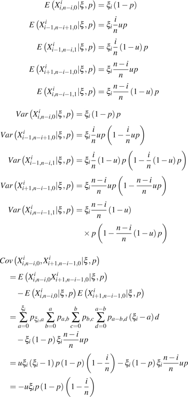where

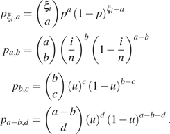Similarly, we have

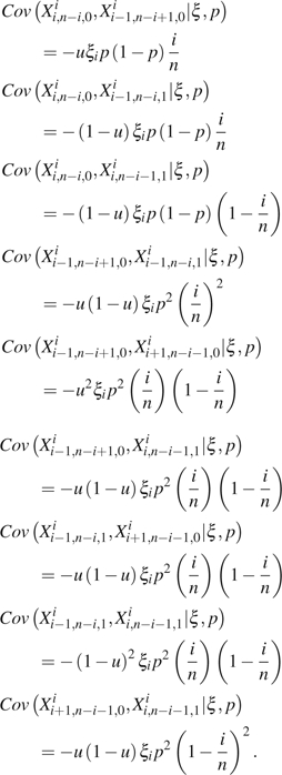Assume all ${\xi }_i$s (represented by ξ) are known. Then, $X_{*}^i$ and $X_{*}^j$ are independent, where * represents any valid configuration and $i\ne j$. So that $Cov(X_{*}^i,X_{*}^j)=0$ when $i\ne j$. Let ${\xi }_{-1}=0$ and ${\xi }_{n+1}=0$, then

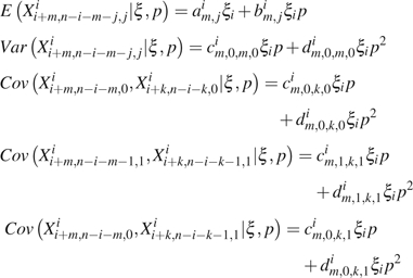where

Then,

Since ${\xi }_i$s are unknown,

References

- Achaz G. Testing for neutrality in samples with sequencing errors. Genetics. 2008;179:1409–1424. doi: 10.1534/genetics.107.082198. [DOI] [PMC free article] [PubMed] [Google Scholar]
- Achaz G, Palmer S, Kearney M, Maldarelli F, Mellors JW, Coffin JM, Wakeley J. A robust measure of HIV-1 population turnover within chronically infected individuals. Mol. Biol. Evol. 2004;21:1902–1912. doi: 10.1093/molbev/msh196. [DOI] [PubMed] [Google Scholar]
- Clark AG, Whittam TS. Sequencing errors and molecular evolutionary analysis. Mol. Biol. Evol. 1992;9:744–752. doi: 10.1093/oxfordjournals.molbev.a040756. [DOI] [PubMed] [Google Scholar]
- Crawford DC, Akey DT, Nickerson DA. The patterns of natural variation in human genes. Annu. Rev. Genomics. Hum. Genet. 2005;6:287–312. doi: 10.1146/annurev.genom.6.080604.162309. [DOI] [PubMed] [Google Scholar]
- Edgar RC. MUSCLE: multiple sequence alignment with high accuracy and high throughput. Nucleic. Acids. Res. 2004;32:1792–1797. doi: 10.1093/nar/gkh340. [DOI] [PMC free article] [PubMed] [Google Scholar]
- Fu YX. A phylogenetic estimator of effective population-size or mutation-rate. Genetics. 1994a;136:685–692. doi: 10.1093/genetics/136.2.685. [DOI] [PMC free article] [PubMed] [Google Scholar]
- Fu YX. Estimating effective population size or mutation rate using the frequencies of mutations of various classes in a sample of DNA sequences. Genetics. 1994b;138:1375–1386. doi: 10.1093/genetics/138.4.1375. [DOI] [PMC free article] [PubMed] [Google Scholar]
- Fu YX. Statistical properties of segregating sites. Theor. Popul. Biol. 1995;48:172–197. doi: 10.1006/tpbi.1995.1025. [DOI] [PubMed] [Google Scholar]
- Fu YX, Li WH. Statistical tests of neutrality of mutations. Genetics. 1993;133:693–709. doi: 10.1093/genetics/133.3.693. [DOI] [PMC free article] [PubMed] [Google Scholar]
- Hellmann I, Mang Y, Gu Z, Li P, de la Vega FM, Clark AG, Nielsen R. Population genetic analysis of shotgun assemblies of genomic sequences from multiple individuals. Genome. Res. 2008;18:1020–1029. doi: 10.1101/gr.074187.107. [DOI] [PMC free article] [PubMed] [Google Scholar]
- Hudson RR. Generating samples under a Wright-Fisher neutral model of genetic variation. Bioinformatics. 2002;18:337–338. doi: 10.1093/bioinformatics/18.2.337. [DOI] [PubMed] [Google Scholar]
- Jiang R, Tavaré S, Marjoram P. Population genetic inference from resequencing data. Genetics. 2009;181:187–197. doi: 10.1534/genetics.107.080630. [DOI] [PMC free article] [PubMed] [Google Scholar]
- Johnson PLF, Slatkin M. Inference of population genetic parameters in metagenomics: a clean look at messy data. Genome. Res. 2006;16:1320–1327. doi: 10.1101/gr.5431206. [DOI] [PMC free article] [PubMed] [Google Scholar]
- Johnson PLF, Slatkin M. Accounting for bias from sequencing error in population genetic estimates. Mol. Biol. Evol. 2008;25:199–206. doi: 10.1093/molbev/msm239. [DOI] [PubMed] [Google Scholar]
- Knudsen B, Miyamoto MM. Incorporating experimental design and error into coalescent/mutation models of population history. Genetics. 2007;176:2335–2342. doi: 10.1534/genetics.106.063560. [DOI] [PMC free article] [PubMed] [Google Scholar]
- Lynch M. Estimation of nucleotide diversity, disequilibrium coefficients, and mutation rates from high-coverage genome-sequencing projects. Mol. Biol. Evol. 2008;25:2409–2419. doi: 10.1093/molbev/msn185. [DOI] [PMC free article] [PubMed] [Google Scholar]
- Mackay T, Richards S, Gibbs R. Proposal to sequence a Drosophila genetic reference panel: a community resource for the study of genotypic and phenotypic variation [white paper]. 2008 FlyBase. org. Available from http://flybase.org/ static_pages/news/wpapers.html. Last accessed on April 14, 2009. [Google Scholar]
- Rosenbaum P, Robertson J, Zamudio K. Unexpectedly low genetic divergences among populations of the threatened bog turtle (Glyptemys muhlenbergii) Conserv. Genet. 2007;8:331–342. [Google Scholar]
- Shendure J, Ji H. Next-generation DNA sequencing. Nat. Biotechnol. 2008;26:1135–1145. doi: 10.1038/nbt1486. [DOI] [PubMed] [Google Scholar]
- Tajima F. Evolutionary relationship of DNA-sequences in finite populations. Genetics. 1983;105:437–460. doi: 10.1093/genetics/105.2.437. [DOI] [PMC free article] [PubMed] [Google Scholar]
- Watterson GA. Number of segregating sites in genetic models without recombination. Theor. Popul. Biol. 1975;7:256–276. doi: 10.1016/0040-5809(75)90020-9. [DOI] [PubMed] [Google Scholar]
- Zhao Z, Jin L, Fu YX, et al. Worldwide DNA sequence variation in a 10-kilobase noncoding region on human chromosome 22. Proc. Natl. Acad. Sci. U.S.A. 2000;97:11354–11358. doi: 10.1073/pnas.200348197. [DOI] [PMC free article] [PubMed] [Google Scholar]
- Zwick ME. A genome sequencing center in every lab. Eur. J. Hum. Genet. 2005;13:1167–1168. doi: 10.1038/sj.ejhg.5201504. [DOI] [PubMed] [Google Scholar]