Problems and Solutions for Estimating Indel Rates and Length Distributions

Abstract

Insertions and deletions (indels) are fundamental but understudied components of molecular evolution. Here we present an expectation–maximization algorithm built on a pair hidden Markov model that is able to properly handle indels in neutrally evolving DNA sequences. From a data set of orthologous introns, we estimate relative rates and length distributions of indels among primates and rodents. This technique has the advantage of potentially handling large genomic data sets. We find that a zeta power-law model of indel lengths provides a much better fit than the traditional geometric model and that indel processes are conserved between our taxa. The estimated relative rates are about 12–16 indels per 100 substitutions, and the estimated power-law magnitudes are about 1.6–1.7. More significantly, we find that using the traditional geometric/affine model of indel lengths introduces artifacts into evolutionary analysis, casting doubt on studies of the evolution and diversity of indel formation using traditional models and invalidating measures of species divergence that include indel lengths.

Introduction

Understanding the origins of spontaneous mutations is critical to the study of molecular biology. Spontaneous mutations are not only the raw material for evolution but also the cause of genetic diseases (Shastry 2007). Using comparative techniques we can measure the relative rates and patterns of neutral mutations and establish the dynamics of spontaneous mutations, including point mutations, insertions, and deletions (Silva and Kondrashov 2002; Britten 2003; Ogurtsov et al. 2004; Lunter 2007). Improved characterization of the mutation process enhances our ability to determine the role of natural selection in molecular evolution (Halpern and Bruno 1998). Furthermore, knowing the dynamics of spontaneous mutations will allow us to improve statistical alignment algorithms, which are a necessary step in many bioinformatic and genomic applications, including phylogenetic tree reconstruction, gene discovery, and protein structure prediction.

Insertions and deletions (indels) are an important component of spontaneous mutations. Recent studies have concluded that indels make up the majority of the divergence among species (Britten 2002, 2003; Anzai et al. 2003; Wetterbom et al. 2006). Although point mutations have been studied extensively, indels have received much less attention. Although studies have found that indel lengths in both DNA and proteins obey a power law (Gonnet et al. 1992; Benner et al. 1993; Gu and Li 1995; Zhang and Gerstein 2003; Chang and Benner 2004; Yamane et al. 2006; Fan et al. 2007), the implications of this finding have been rarely explored (but see Cartwright 2006; Kim and Sinha 2007). It is important to study the diversity of indel processes on the tree of life because changes in the processes can reveal functional changes in core DNA replication and repair enzymes. Additionally, knowing where the indel process is conserved allows us to use constant parameters in alignment models for these areas. And importantly, when comparing indel rates and length distributions among branches in the tree of life, estimation procedures should not introduce artifacts.

Typical studies of spontaneous indels take orthologous sequences in two species, construct their alignment, and then estimate the rate and length distribution from these alignments, for example, Rat Genome Sequencing Project Consortium (2004). However, these alignments are not perfect; Lunter et al. (2008) find that whole-genome alignments between species as divergent as humans and mice will wrongly align at least 10% of the residues. Additionally, because one must usually choose alignment models and scoring schemes ahead of time, such alignments are generated using assumptions about the nature of the spontaneous mutation process and often fit the assumptions better than reality; they are “too good.” Clearly, this approach is circular—like using guide trees to construct multiple sequence alignments for phylogenetic reconstruction (Lake 1991; Thorne and Kishino 1992; Redelings and Suchard 2005)—and there is potential for alignments to introduce artifacts into the estimated rates, especially for taxa that are distantly related and difficult to align (Metzler et al. 2001; Metzler 2003; Lunter 2007; Lunter et al. 2008). For example, biases in alignment algorithms have been shown to decrease estimates of indel rates (Lunter 2007; Lunter et al. 2008), and failure to account for indels in an evolutionary context introduces errors in progressive alignments that impact evolutionary analysis (Löytynoja and Goldman 2008).

To avoid circularity, one should estimate indel processes from unaligned, orthologous sequences. In this alignment-free approach, estimates are produced by averaging over all possible alignments between sequences, eliminating biases introduced by using only the “best” alignment and allowing alignment uncertainty to improve rate estimates. Whereas posterior decoding approaches address the same problem but use all possible alignments to exclude sections that are uncertain from further analysis (e.g., Durbin et al. 1998; Lunter et al. 2008), our approach incorporates uncertain regions in inference.

However, even after eliminating alignment artifacts, comparisons may still contain artifacts if an unrealistic model of indel formation is used. Although an unrealistic model may have enough power for inference, this is not always the case and there are good reasons to suspect that traditional models of indel formation produce estimation artifacts that make inference problematic. Traditionally, indel length distributions are assumed to obey a computationally tractable geometric distribution (the affine gap model, Gotoh 1982), although recently mixture-of-geometric distributions have been explored (Miklós et al. 2004; Lunter 2007; Lunter et al. 2008). However, as pointed out above, many empirical studies have found a power-law relationship between indel length and frequency. We will represent this relationship with a zeta distribution, which is a discrete distribution defined on integers [1, ∞) that obeys a power law. In a zeta, the probability that an indel has length k is k^−z/ζ(z), where z > 1 and ζ is Riemann's Zeta function. If z ≤ 2, the mean is infinite, and if z ≤ 3, the variance is infinite. Note that if indel lengths follow a zeta distribution, then sequences should be probabilistically aligned using log-affine gap costs, a + bk + c ln k, instead of the affine gap model (Cartwright 2006).

Previous studies suggest that indel length distributions obey power laws with z < 2 (Gu and Li 1995; Zhang and Gerstein 2003; Yamane et al. 2006; Fan et al. 2007). Although, a sample from such zeta distributions will have a finite average, the variance of the sample average will still be infinite (or nearly so, assuming a finite upper bound imposed by selection and genome length). Thus, two independent samples from the same distribution are prone to having different averages, and they will converge slowly or not at all upon increasing sample size. This is true for estimates from different taxa as well as estimates from different chromosomes. Therefore, if indels truly follow zeta distributions, we should not expect primate introns to have the same average length as rodent introns even when both groups were sampled from the same distribution because the sample variance is (nearly) infinite. To avoid such artifacts, we will estimate indel length distributions using a zeta-based model.

Following Holmes (2005), we employ expectation–maximization (EM) to obtain parameter estimates and their approximate variances (Dempster et al. 1977; Louis 1982) for the pair hidden Markov model (HMM) of alignments described below. Unlike early attempts of estimating indel rates and length distributions using data sets of pseudogene alignments (Gu and Li 1995; Ophir and Graur 1997; Zhang and Gerstein 2003), our data set consists of unaligned orthologous introns from primate and rodent genomes. Under the assumption that these introns have evolved neutrally, our between-species estimates of substitution rates should approximate intraspecies spontaneous mutation rates. We compare both geometric and zeta models of indel length and find that a zeta provides a significantly better model for indel length distributions. Furthermore, we find that spontaneous indel processes appear to be conserved between rodents and primates. Importantly, we demonstrate that using a geometric model for indel lengths produces artifacts. To help researchers explore statistical alignment strategies, our evolutionary alignment models have been implemented in version 1.2 of our Ngila software (Cartwright 2007).

Materials and Methods

Generalized Pair HMM Architecture

We model pairwise alignments via a pair HMM (Durbin et al. 1998), called SMUVE after the node labels (fig. 1). Like Knudsen and Miyamoto (2003), Holmes (2005), Wang et al. (2006), Metzler et al. (2001), and Metzler (2003), our alignments are modeled as unobserved data that emit a pair of “observed” sequences. We developed SMUVE to be as biologically realistic as possible while maintaining computational tractability. Our most important concern was limiting the amount of memory needed to estimate parameters for SMUVE models. This is reflected in choices made in our HMM architecture and our substitution model.

FIG. 1.—

SMUVE, a generalized pair HMM architecture. Match state (M) emits a pair of nucleotides to the alignment via the K2P model, whereas indel states (U and V) emit nucleotides to only one sequence based on either a zeta or geometric distribution. Transition probabilities are evenly distributed out of each node unless otherwise noted; τ = 1/(a + 1) and η = e^−2rt.

Conceptually, we distinguish gaps from indels; an indel is a specific evolutionary event that adds or removes residues from a sequence, whereas a gap results from one or more overlapping or adjoining indels making residues in one sequence nonhomologous to any residues in the other sequence. Furthermore, an indel in one sequence can be caused by a deletion that occurred in its lineage or an insertion that occurred in the other lineage. Thus, length distributions of indels are a mixture of an insertion length distribution and a deletion length distribution, and length distributions of gaps are a complex summation of indel length distributions. Although some previous studies have used outgroups or pseudogenes to distinguish insertions from deletions (Gu and Li 1995; Ophir and Graur 1997; Zhang and Gerstein 2003; Fan et al. 2007; Matthee et al. 2007), such techniques would make SMUVE slower or restrict the type of data that it can handle. We will defer separating insertions from deletions to another study and assume here that indels have the same rate of occurrence as well as the same length distribution (cf. Knudsen and Miyamoto 2003; Metzler 2003; Wang et al. 2006; Lunter 2007; Lunter et al. 2008). This simplifies our HMM and resolves insertion and deletion processes into a single, easily handled indel process.

SMUVE has five different hidden states: start (S), two-residue homology (M), indel in one sequence (U), indel in the other sequence (V), and end (E). However unlike other pair HMMs (Knudsen and Miyamoto 2003; Holmes 2005; Wang et al. 2006), SMUVE is a generalized HMM that emits indels in blocks of random lengths, which is necessary for implementing zeta distributions of indel lengths. In a sense, our hidden Markov chain is not the actual alignment, but a skeleton on which the alignment is constructed. In our model, the transitions between M, U, and V are independent, which simplifies the analysis of the model and reduces its memory usage. We also make the simplifying assumption to ignore overlapping indels while allowing neighboring indels. Our desire to analyze a zeta model precludes the use of techniques to handle overlapping indels (Knudsen and Miyamoto 2003; Miklós et al. 2004).

Given that the chain does not terminate, the probability that the next state in the chain is M is η = e^−2rt, where t is the evolutionary distance between the two sequences measured in expected number of substitutions per orthologous residue pair. If indel formation is a Poisson process with relative rate 2r (times the substitution rate), then η is the probability that no indel has occurred at a specific site in either lineage separated by distance t (Knudsen and Miyamoto 2003). Likewise, given that the chain does not terminate, the probabilities of U and V are both (1 − η)/2. The instantaneous rates of k-residue indels (λ_k, μ_k) are simply the instantaneous rate of the Poisson process, times the length distribution—λ_k = μ_k = rtf_k(k)—which are comparable to the instantaneous rates used in other formulations of evolutionary indel models (e.g., Miklós et al. 2004).

To ensure that SMUVE is a proper HMM, we introduce a nuisance parameter that governs the probability that the chain terminates. This parameter, a, is the expected length of the M, U, and V skeleton, and the probability that the alignment chain terminates at any point in time is τ = 1/(a + 1). The nuisance parameter has very little impact on the overall likelihood of the model and some HMMs ignore it (Knudsen and Miyamoto 2003; Wang et al. 2006). Biologically, a is related to the length of the ancestral sequence and the indel process. Although, a parameter for the ancestral sequence length would be biologically informative, it is not trivial to disentangle it from the indel process.

We implemented two different versions of SMUVE: geo-SMUVE, which emits indels using a geometric length distribution, and zeta-SMUVE, which emits indels using a zeta length distribution. We did not implement a version using a mixture-of-geometric-distributions (Miklós et al. 2004; Lunter 2007; Lunter et al. 2008) because although both zeta and geometric distributions require only a single parameter, a mixture of geometrics requires at least 3 parameters and still underweights large indels. Both SMUVE versions emit nucleotide residues using the Kimura 2-parameter model (K2P, Kimura 1980), which has a time parameter, t, and transition–transversion ratio, k. K2P is more realistic than the Jukes–Cantor model (Jukes and Cantor 1969) but does not require as many summary statistics as more complex models. By avoiding more complex models, we retain the ability to analyze longer, more interesting sequences. Nucleotides are emitted by indel states based on K2P's stationary frequency, which is 1/4.

Sequence Data

Six orthologous serpin (Law et al. 2006) gene sequences were downloaded from GenBank via the HomoloGene database for each of four species: Homo sapiens, Pan troglodytes, Mus musculus, and Rattus norvegicus. The download included both confirmed and predicted genes. Many chimp sequences and some rat sequences had multiple predicted intron–exon configurations at the time of the download. When this was the case, the order that agreed best with the human and mouse orders was chosen by eye. GenBank and FASTA formatted sequences can be found in Supplementary Material online.

Sets of orthologous introns within coding regions were extracted from this data. We did not exclude regions of the introns that are selected to maintain proper excision; however, their contribution should be minor in the data set. For computational efficiency, these sets were further pruned by excluding any orthologous set in which at least one intron had a length greater than 2,500 residues. This also helps to avoid genes or microRNAs that may reside within larger introns. Each genome was represented by approximately 12,000 residues in the final data set, which contained 11 introns: SERPINA3 intron 3, SERPINA6 intron 3, SERPINA8 introns 2 and 3, SERPINH1 introns 1 and 2, SERPINI1 introns 2, 6, and 7, and SERPINI2 introns 2 and 3. (Note that intron 1 is the intron after the first coding exon in our scheme.)

Maximum Likelihood Estimators

If the true alignment of sequences X and Y was known, then our model has a trivial solution to the maximum likelihood formula

(1)

where θ represents the set of model parameters and A represents the homology indel spectrum of the alignment. For zeta-SMUVE, θ = {t, k, a, r, z}, and for geo-SMUVE, θ = {t, k, a, r, q}. Substitution parameters $\widehat{t}$ and $\widehat{k}$ can be estimated via the K2P solutions (Kimura 1980). The maximum likelihood estimate (MLE) solutions for the rest of the parameters are as follows:

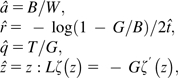(2)

where W is the number of sequence pairs in the data set, B is the number of matches, mismatches, and indels in the alignment, G is the number of indels, T is the sum of the indel lengths, and L is the sum of the log of indel lengths. (These were calculated by finding the root of the first derivative of the log likelihood and numerically confirmed by our analysis algorithm.)

Expectation–Maximization

However, in our and nearly all data sets, the true alignment is actually unknown; it is missing data. Here MLE is considerably more complicated because we must marginalize over the unknown alignment

(3)

To simplify things, we employ EM (Dempster et al. 1977) to use the solution of equation (1) to solve equation (3).

EM is an iterative method of doing MLE with missing data. From an initial guess, θ₀, the parameters are updated via a two-step method until the log likelihood converges to a local maximum. The E-step calculates a function, Q(θ |θ_n), where

and the M-step maximizes this function with respect to θ, giving the next estimate of θ

EM not only allows us to estimate evolutionary parameters for indel models in a noncircular manner, it also allows us to use orthologous sequences for which homology is difficult to assign to individual sites, in contrast to other methods, for example, Ogurtsov et al. (2004). We can also directly estimate the variance of MLEs, avoiding time-consuming techniques like bootstrapping (Louis 1982).

We implemented EM analysis algorithms for both geo-SMUVE and zeta-SMUVE models in a C++ application, which is available on request. The likelihood calculations of both models were properly proportioned to allow comparisons between them. For the E-step, dynamic programming was used to take the expected values of the summary statistics over all possible alignments. The zeta-SMUVE analysis had a time complexity on sequence length of O(N³) because the zeta distribution does not allow alignment lookbacks to be cached. However, we did implement caching for the geo-SMUVE analysis, which reduced the complexity to O(N²). We combined the expectations of each sequence pair in the data set and then maximized the likelihood on the total. This means that parameter a has even less biological relevance because it is the average skeleton length of several independent sequence pairs.

Geo-SMUVE and zeta-SMUVE parameters were estimated for all six species–species pairs. For the human–mouse comparison, the initial parameters of the geo-SMUVE estimation were t = 0.1, k = 2.0, a = 1,000, r = 0.1, and q = 10, and for zeta-SMUVE they were t = 0.48, k = 1.5, a = 1,000, r = 0.1, and z = 1.6. For mouse–rat, they were t = 0.17, k = 2.0, a = 1,000, r = 0.0629, and q = 6.905—and t = 0.16, k = 2.0, a = 1,000, r = 0.1, and z = 1.7. We considered the EM to have converged when the change in log likelihood was less than 10⁻⁵. We used the MLEs from the human–mouse comparison to serve as initial parameter values for the remaining species–species pairs, except that t = 0.02 for the human–chimp analysis.

The method of Louis (1982) was solved in Mathematica (Wolfram Research, Inc. 2007) to generate equations for finding the covariance matrix of the MLEs. We implemented these equations in our application and then calculated the covariance matrices for our data sets and converged MLEs.

To calculate histograms for the observed length distribution of indels in the sequences, we adapted our dynamic programming algorithm to estimate, over all possible alignments, the average and variance of the number of indels of specific sizes. We then ran these modified algorithms at the converged MLEs.

Simulations

To compare the EM estimation procedure with optimal alignment estimation, we generated 100 sets of 11 sequence pairs under both geo-SMUVE and zeta-SMUVE HMM models for six different divergences, t ∈ {0.01, 0.05, 0.15, 0.3, 0.45, 0.6}. For the rest of the parameters, we used the human–mouse estimates reported below for these models, and we excluded sequence pairs that were smaller or larger than those in our biological data set. For the optimal approach, we found the best alignment under the simulated model via Ngila (Cartwright 2007) and then estimated model parameters from the alignments for each sequence pair. For the EM approach, we used the implementation mentioned above with the initial parameters being the simulation parameters.

Results

Figure 2 displays both the root mean squared errors (RMSE) and the biases of optimal and EM estimation procedures as calculated from our simulations. All four procedures do fairly well when estimating branch lengths and Ts/Tv ratios, having low RMSE and biases. However, geo-optimal and zeta-optimal show considerable increase in RMSE of indel rate and length parameter estimates as sequence divergence increase. Additionally, alignment optimization introduced biases that decreased the estimated indel rates and increased the lengths of indels (cf. Lunter 2007; Lunter et al. 2008). In contrast, geo-SMUVE and zeta-SMUVE show no comparable increase in error or bias as divergence increases.

FIG. 2.—

Comparison of optimal and EM estimation procedures. Each line represents one of four procedures: geo-SMUVE, geometric optimal, zeta-SMUVE, and zeta-optimal. RMSE and biases have been normalized using the true value of the parameters. Note that the indel length distribution parameters of the geometric and zeta models are not directly comparable to one another.

We estimated evolutionary parameters from a set of orthologous introns from the human, chimp, mouse, and rat genomes. For each pair, we used both zeta-SMUVE and geo-SMUVE and estimated the distance (t), Ts/Tv ratio (k), relative indel rate (r), and the length distribution parameter: either the zeta's slope magnitude (z) or the geometric's mean (q). Results can be found in figure 3. Regardless of the species–species pair, we find that t, k, and r are statistically indistinguishable between both models. (Note that z and q are not directly comparable.) Additionally, k, r, and z are conserved across all taxa, whereas q is not. Because q is estimated from the average indel length, we expect that artifacts will make q unconserved. Our estimated species divergences are consistent with previous work (Chen and Li 2001; Mouse Genome Sequencing Consortium 2002; The Chimpanzee Sequencing and Analysis Consortium 2005), as are our estimates for the magnitude of the zeta's slope (Gu and Li 1995; Zhang and Gerstein 2003; Fan et al. 2007). Our estimated relative indel rates agree with the higher rate found by a recent probabilistic study (Lunter 2007) and disagree with earlier, lower rates found by alignment-based studies (Silva and Kondrashov 2002; Britten 2003; Ogurtsov et al. 2004). Note that human–chimp estimates have larger variances because they have fewer evolutionary differences.

FIG. 3.—

Estimated maximum likelihood SMUVE parameters, with 95% confidence intervals. Each bar is an estimate from a pairwise comparison among human, chimp, mouse, or rat. Distribution parameters are not directly comparable between the two models and are plotted on different axes.

According to table 1, modeling indel distributions with a zeta distribution provides a huge increase in the likelihood of the final estimates. The smallest increase is for the human–chimp comparison, but the best zeta model is still 1.5 × 10¹⁵ times more likely than the best geometric model. This difference is due to the fact that the predicted indel length distributions are very different between the zeta and geometric models. For instance, the traditional geometric model predicts that 15% of the indels between rats and mice should be of length 1, whereas the zeta model predicts that 49% of them are.

Table 1.

Natural Log Likelihoods of SMUVE Results

Comparison	Zeta	Geometric	Likelihood Ratio
Human–Chimp	−19,456	−19,490	1.5 × 1015 : 1
Mouse–Rat	−24,543	−24,621	2.0 × 1034 : 1
Human–Mouse	−32,381	−32,513	2.1 × 1057 : 1
Human–Rat	−31,601	−31,736	4.2 × 1058 : 1
Chimp–Rat	−32,176	−32,319	1.3 × 1062 : 1
Chimp–Mouse	−32,958	−33,110	3.8 × 1065 : 1

To further investigate the differences between the zeta MLEs and the geometric MLEs, we ran SMUVE again on the mouse–rat data set and measured the observed number of indels of length 1–9 per alignment at convergence. This allows us to investigate the most likely alignment space of our sequences. The results are in figure 4 and are plotted along with triangles that represent the MLEs of length distributions. If the histograms differ from the estimates, then matches in the sequences contain information about the location and length of indels that the indel length distribution is not capturing. The zeta model appears to be a good fit to the data, whereas the geometric has a hard time capturing the head and the tail of the histogram.

FIG. 4.—

Histograms of the observed number of indels of lengths 1–9 in the mouse–rat alignment space, with 95% confidence intervals. Triangles represent MLEs.

As an example of the differences between zeta-SMUVE and geo-SMUVE alignments, we compare the alignment precision of both models for human and mouse SERPINA3, intron 3 in figures S.1 and S.2 (Supplementary Material online). Using posterior decoding of 10,000 alignments sampled from each model (Durbin et al. 1998; §4.4), we found the most consistent alignment given by each model at our estimated MLE parameters. The models produce different posterior decoded alignments; zeta-SMUVE favors more matches and less gapped residues and produces an alignment with higher consistency, indicating that its alignment space is less ambiguous.

Discussion

We have developed an alignment-free method of estimating indel rates and length distributions and estimated two models on a data set consisting of orthologous introns from human, chimp, mouse, and rat genomes. Our results demonstrate that EM procedures perform better than optimal alignment procedures for estimating evolutionary models from divergent taxa. Additionally, EM avoids the necessity of specifying optimal alignment criteria when lacking knowledge about the biological parameters. In this sense, the errors and biases in figure 2 are actually smaller than they would typically be in practice because we found optimal alignments under the simulated model and did not guess at the alignment parameters. By averaging over all possible alignments, EM in some sense finds marginal alignments, which are considerably more accurate than optimal alignments in representing the evolutionary history of two sequences. This further suggests that the best alignment for summarizing the evolutionary history of two orthologous sequences is not the optimal alignment but rather the alignment that best fits marginal summary statistics.

Zeta Power-Law Superiority

Our results demonstrate that a zeta model produces fewer artifacts and better describes the distribution on indel lengths in our data set than the classic geometric model (cf. Gonnet et al. 1992; Benner et al. 1993; Gu and Li 1995; Zhang and Gerstein 2003; Chang and Benner 2004; Yamane et al. 2006; Fan et al. 2007). Additionally, a zeta model produced a more consistent posterior decoded alignment than a geometric model in our supplementary example. Although a zeta model provides a better fit, we have not proved that indels truly have a zeta length distribution. Several biological processes create indels, each having their own length distributions and favored locations for formation. Short indels are mostly caused by polymerase slippage during replication and often occur in repeat regions. Moderate to large indels are rarer and are caused by nonhomologous recombination and transposon activity. And as mentioned above, an indel can be either an insertion or a deletion, each type potentially having its own rate and length distribution. However, it might be difficult for a model to detect a rare process that produces large indels because the big weight of a zeta's tail could potentially hide these events. Simply put, the model would not see them as exceptional or outliers.

Besides the superiority of the zeta model, our analysis confirmed that estimates for the geometric model were not conserved between rodents and primates, whereas estimates for the zeta model were. The nonconservation of average indel length means that it is very difficult to study the evolution of indel-length distributions using geometric models. Additionally, this nonconservation invalidates measures of species divergence that count indel lengths (Britten 2002, 2003). Although the total number of indels is proportional to the number of substitutions separating species, the total length of indels is unrelated to divergence. Therefore, we should use established metrics of divergence, like the expected number of substitutions, and avoid being seduced by indel length metrics. Additionally, because zeta-SMUVE is conserved across the taxa studied, it is possible to use a common set of parameters to find optimal alignments or phylogenies between sequences in these taxa, adjusting only the evolutionary distance between each pairing.

The best-fitting geometric and zeta distributions give us strikingly different inferences. For instance, if we calculate the frequency of single nucleotide gaps from our estimated parameters, the zeta model predicts that they make up 39% of the indels between humans and chimps, whereas the geometric only predicts 2%. Between mice and humans, these numbers are 46% and 6% and between mice and rats, 49% and 14%. Furthermore, the zeta estimates all agree that the median indel length should be less than 2; however, the geometric models put the median lengths anywhere from 4 to 34 residues long (data not shown). Thus, by using geometric models, we tend to undervalue single-residue indels, causing a conflict between our data and alignment models, as seen in figure 4.

Interestingly, although we find that zeta and geometric models perform differently, we did not find any significant differences between the two models in parameter estimates of sequence divergence, Ts/Tv ratio, or relative indel rate. This suggests that both models were equally successful in locating gapped and ungapped regions in our data set but differed in their abilities to fit the gapped regions. Although not equivalent to the marginal likelihood of our sequences, we can calculate a likelihood from our marginal summary statistics to approximately determine the influence of the indel length distributions on the total likelihood. Doing this on our human–mouse data set, we find that the length distributions contribute roughly 4.2% and 5.5% of the zeta-SMUVE and geo-SMUVE likelihoods, respectively, whereas substitutions and stationary residue frequencies contribute the vast majority, >85%, of the likelihoods. These results suggest that if one is not concerned with estimating indel length distributions, then there is little difference in estimation performance between the zeta-SMUVE and the faster geo-SMUVE.

Limitations

Despite its strengths, the model has important limitations. The most notable is the cubic time and squared memory complexity of the zeta-SMUVE model, which dictated several concessions to the model. These concessions include the use of the K2P substitution model over the more flexible general time reversible model, the independent state transitions in the hidden Markov chain, and the exclusion of introns over 2,500 residues long. We also ignored variation in GC content between introns; however, with a larger, full-genome data set, it would be possible to bin introns based on GC content or other criteria and estimate indel models for each bin (cf. Lunter 2007; Lunter et al. 2008).

Unlike two other studies (Knudsen and Miyamoto 2003; Miklós et al. 2004), SMUVE makes no attempts to handle overlapping indels other than summing over all possible consecutive indels. For closely related species, overlapping indels are probably rare and this is not a concern; however, when we use our human–mouse zeta-SMUVE estimates in the equations of Knudsen and Miyamoto (2003), we estimate that 3.3% of sites that experience indels will be hit a second time. Of these, 1/4 will be an insertion followed by a deletion, which we do not properly handle. In fact, using our estimated zeta length distribution, which heavily favors single nucleotide indels, we can estimate that 24% of all deleted insertions will leave no trace of either event. These are conservative calculations of the unmeasured effects of indel overlap because they do not consider indel overlap between large events at distant sites. However, the minor errors introduced by unmeasured overlapping indels into our estimates should be well within their 95% confidence intervals.

Furthermore, our estimation model does not distinguish insertions from deletions, whereas several empirical studies have found differences between the rates of indels (Gu and Li 1995; Ophir and Graur 1997; Zhang and Gerstein 2003; Fan et al. 2007; Matthee et al. 2007). We are working on an SMUVE derivative that is not only able to separate indels but is also able to estimate the placement of the common ancestor of two sequences. Once we can estimate the rates and length distributions of indels separately, we can not only compare these processes but also start adapting the SMUVE model to multiple sequences.

Future Directions

Our eventual goal is to apply SMUVE to study the diversity and evolution of indel rates and length distributions over the tree of life. We will not only be able to explore how substitutions in DNA replication and repair enzymes may be associated with changes in the indel process, but we will also determine the optimal method for aligning sequences from each taxon. The algorithm is keenly suited for comparative genomic studies on pairs of species because it is trivial to pool data across orthologous regions, which also makes parallelization and distributed programming optimizations straightforward to implement. However, SMUVE's complexity will need to be reduced for applications of this magnitude because it is limited strongly by the maximum sequence length of a data set. We can also speed computation through a stepping-stone algorithm that can distinguish regions with obvious alignments from regions with ambiguous alignments (Meyer and Durbin 2002). That way we only process smaller subsequences of introns. We have used this approach already by relying on exons to anchor introns. Other promising techniques are also currently in development.

Although, improving SMUVE's speed is important in order to apply it to large, whole-genome data sets, ensuring that those data sets are of high quality is of equal or greater importance. In this study, our data set consisted of orthologous introns gathered from a curated database of orthologous genes. Creating a similar data set on a large scale, from uncurated sources, and perhaps including genomes from poorly understood species would take a lot of creativity and is a project in its own right.

Conclusion

We have demonstrated the utility of statistical alignments and EM to estimate indel rates and length distributions from genomic data and confirmed the existence of artifacts produced by traditional, geometric models. The inherent nonconservation of geometric models estimated from zeta-distributed data makes it impossible to study the evolution and diversity of indel formation using traditional models. A zeta length distribution or some derivative of it needs to be used in order to have enough power to test hypotheses about indel length distributions.

Supplementary Material

Supplementary figures S.1 and S.2 and the sequence data used in this paper are available at Molecular Biology and Evolution online (http://www.mbe.oxfordjournals.org/).

References

- Anzai T, Shiina T, Kimura N, et al. (21 co-authors) Comparative sequencing of human and chimpanzee MHC class I regions unveils insertions/deletions as the major path to genomic divergence. Proc Natl Acad Sci USA. 2003;100:7708–7713. doi: 10.1073/pnas.1230533100. [DOI] [PMC free article] [PubMed] [Google Scholar]
- Benner SA, Cohen MA, Gonnet GH. Empirical and structural models for insertions and deletions in the divergent evolution of proteins. J Mol Biol. 1993;229:1065–1082. doi: 10.1006/jmbi.1993.1105. [DOI] [PubMed] [Google Scholar]
- Britten RJ. Divergence between samples of chimpanzee and human DNA sequences is 5%, counting indels. Proc Natl Acad Sci USA. 2002;99:13633–13635. doi: 10.1073/pnas.172510699. [DOI] [PMC free article] [PubMed] [Google Scholar]
- Britten RJ. Majority of divergence between closely related DNA sequences is due to indels. Proc Natl Acad Sci USA. 2003;100:4661–4665. doi: 10.1073/pnas.0330964100. [DOI] [PMC free article] [PubMed] [Google Scholar]
- Cartwright RA. Logarithmic gap costs decrease alignment accuracy. BMC Bioinformatics. 2006;7:527. doi: 10.1186/1471-2105-7-527. [DOI] [PMC free article] [PubMed] [Google Scholar]
- Cartwright RA. Ngila: global pairwise alignments with logarithmic and affine gap costs. Bioinformatics. 2007;23:1427–1429. doi: 10.1093/bioinformatics/btm095. [DOI] [PMC free article] [PubMed] [Google Scholar]
- Chang MSS, Benner SA. Empirical analysis of protein insertions and deletions determining parameters for the correct placement of gaps in protein sequence alignments. J Mol Biol. 2004;341:617–631. doi: 10.1016/j.jmb.2004.05.045. [DOI] [PubMed] [Google Scholar]
- Chen F-C, Li W-H. Genomic divergences between humans and other hominoids and the effective population size of the common ancestor of humans and chimpanzees. Am J Hum Genet. 2001;68:444–456. doi: 10.1086/318206. [DOI] [PMC free article] [PubMed] [Google Scholar]
- Dempster AP, Laird NM, Rubin DB. Maximum likelihood from incomplete data via the EM algorithm. J R Stat Soc Ser B (Methodol) 1977;39:1–38. [Google Scholar]
- Durbin R, Eddy S, Krogh A, Mitchinson G. Biological sequence analysis. Cambridge University Press. Cambridge (UK); 1998. [Google Scholar]
- Fan Y, Wang W, Ma G, Liang L, Shi Q, Tao S. Patterns of insertion and deletion in mammalian genomes. Curr Genomics. 2007;8:370–378. doi: 10.2174/138920207783406479. [DOI] [PMC free article] [PubMed] [Google Scholar]
- Gonnet GH, Cohen MA, Benner SA. Exhaustive matching of the entire protein sequence database. Science. 1992;256:1443–1445. doi: 10.1126/science.1604319. [DOI] [PubMed] [Google Scholar]
- Gotoh O. An improved algorithm for matching biological sequences. J Mol Biol. 1982;162:705–708. doi: 10.1016/0022-2836(82)90398-9. [DOI] [PubMed] [Google Scholar]
- Gu X, Li WH. The size distribution of insertions and deletions in human and rodent pseudogenes suggests the logarithmic gap penalty for sequence alignment. J Mol Evol. 1995;40:464–473. doi: 10.1007/BF00164032. [DOI] [PubMed] [Google Scholar]
- Halpern A, Bruno W. Evolutionary distances for protein-coding sequences: modeling site-specific residue frequencies. Mol Biol Evol. 1998;15:910–917. doi: 10.1093/oxfordjournals.molbev.a025995. [DOI] [PubMed] [Google Scholar]
- Holmes I. Using evolutionary expectation maximization to estimate indel rates. Bioinformatics. 2005;21:2294–2300. doi: 10.1093/bioinformatics/bti177. [DOI] [PMC free article] [PubMed] [Google Scholar]
- Jukes TH, Cantor CR. Evolution of protein molecules. In: Munro HN, editor. Mammalian protein metabolism, volume 3. New York: Academic Press; 1969. pp. 21–132. [Google Scholar]
- Kim J, Sinha S. Indelign: a probabilistic framework for annotation of insertions and deletions in a multiple alignment. Bioinformatics. 2007;23:289–297. doi: 10.1093/bioinformatics/btl578. [DOI] [PubMed] [Google Scholar]
- Kimura M. A simple method for estimating evolutionary rates of base substitutions through comparative studies of nucleotide-sequences. J Mol Evol. 1980;16:111–120. doi: 10.1007/BF01731581. [DOI] [PubMed] [Google Scholar]
- Knudsen B, Miyamoto MM. Sequence alignments and pair hidden Markov models using evolutionary history. J Mol Biol. 2003;333:453–460. doi: 10.1016/j.jmb.2003.08.015. [DOI] [PubMed] [Google Scholar]
- Lake JA. The order of sequence alignment can bias the selection of tree topology. Mol Biol Evol. 1991;8:378–385. doi: 10.1093/oxfordjournals.molbev.a040654. [DOI] [PubMed] [Google Scholar]
- Law RH, Zhang Q, McGowan S, et al. (11 co-authors) An overview of the serpin superfamily. Genome Biol. 2006;7:216. doi: 10.1186/gb-2006-7-5-216. [DOI] [PMC free article] [PubMed] [Google Scholar]
- Louis TA. Finding the observed information matrix when using the EM algorithm. J R Stat Soc Ser B (Methodol) 1982;44:226–233. [Google Scholar]
- Löytynoja A, Goldman N. Phylogeny-aware gap placement prevents errors in sequence alignment and evolutionary analysis. Science. 2008;320:1632–1635. doi: 10.1126/science.1158395. [DOI] [PubMed] [Google Scholar]
- Lunter G. Probabilistic whole-genome alignments reveal high indel rates in the human and mouse genomes. Bioinformatics. 2007;23:i289–i296. doi: 10.1093/bioinformatics/btm185. [DOI] [PubMed] [Google Scholar]
- Lunter G, Rocco A, Mimouni N, Heger A, Caldeira A, Hein J. Uncertainty in homology inferences: assessing and improving genomic sequence alignment. Genome Res. 2008;18:298–309. doi: 10.1101/gr.6725608. [DOI] [PMC free article] [PubMed] [Google Scholar]
- Matthee CA, Eick G, Willows-Munro S, Montgelard C, Pardini AT, Robinson TJ. Indel evolution of mammalian introns and the utility of non-coding nuclear markers in eutherian phylogenetics. Mol Phylogenet Evol. 2007;42:827–837. doi: 10.1016/j.ympev.2006.10.002. [DOI] [PubMed] [Google Scholar]
- Metzler D. Statistical alignment based on fragment insertion and deletion models. Bioinformatics. 2003;19:490–499. doi: 10.1093/bioinformatics/btg026. [DOI] [PubMed] [Google Scholar]
- Metzler D, Fleißner R, Wakolbinger A, von Haeseler A. Assessing variability by joint sampling of alignments and mutation rates. J Mol Evol. 2001;53:660–669. doi: 10.1007/s002390010253. [DOI] [PubMed] [Google Scholar]
- Meyer IM, Durbin R. Comparative ab initio prediction of gene structures using pair HMMs. Bioinformatics. 2002;18:1309–1318. doi: 10.1093/bioinformatics/18.10.1309. [DOI] [PubMed] [Google Scholar]
- Miklós I, Lunter G, Holmes I. A “long indel” model for evolutionary sequence alignment. Mol Biol Evol. 2004;21:529–540. doi: 10.1093/molbev/msh043. [DOI] [PubMed] [Google Scholar]
- Mouse Genome Sequencing Consortium. Initial sequencing and comparative analysis of the mouse genome. Nature. 2002;420:520–526. doi: 10.1038/nature01262. [DOI] [PubMed] [Google Scholar]
- Ogurtsov AY, Sunyaev S, Kondrashov AS. Indel-based evolutionary distance and mouse-human divergence. Genome Res. 2004;14:1610–1616. doi: 10.1101/gr.2450504. [DOI] [PMC free article] [PubMed] [Google Scholar]
- Ophir R, Graur D. Patterns and rates of indel evolution in processed pseudogenes from humans and murids. Gene. 1997;205:191–202. doi: 10.1016/s0378-1119(97)00398-3. [DOI] [PubMed] [Google Scholar]
- Rat Genome Sequencing Project Consortium. Genome sequence of the Brown Norway rat yields insights into mammalian evolution. Nature. 2004;428:493–521. doi: 10.1038/nature02426. [DOI] [PubMed] [Google Scholar]
- Redelings B, Suchard M. Joint Bayesian estimation of alignment and phylogeny. Syst Biol. 2005;54:401–418. doi: 10.1080/10635150590947041. [DOI] [PubMed] [Google Scholar]
- Shastry BS. SNPs in disease gene mapping, medicinal drug development and evolution. J Hum Genet. 2007;52:871–880. doi: 10.1007/s10038-007-0200-z. [DOI] [PubMed] [Google Scholar]
- Silva JC, Kondrashov AS. Patterns in spontaneous mutation revealed by human-baboon sequence comparison. Trends Genet. 2002;18:544–547. doi: 10.1016/s0168-9525(02)02757-9. [DOI] [PubMed] [Google Scholar]
- The Chimpanzee Sequencing and Analysis Consortium. Initial sequence of the chimpanzee genome and comparison with the human genome. Nature. 2005;437:69–87. doi: 10.1038/nature04072. [DOI] [PubMed] [Google Scholar]
- Thorne JL, Kishino H. Freeing phylogenies from artifacts of alignment. Mol Biol Evol. 1992;9:1148–1162. doi: 10.1093/oxfordjournals.molbev.a040783. [DOI] [PubMed] [Google Scholar]
- Wang J, Keightley PD, Johnson T. MCALIGN2: faster, accurate global pairwise alignment of non-coding DNA sequences based on explicit models of indel evolution. BMC Bioinformatics. 2006;7:292. doi: 10.1186/1471-2105-7-292. [DOI] [PMC free article] [PubMed] [Google Scholar]
- Wetterbom A, Servov M, Cavelier L, Bergström TF. Comparative genomic analysis of human and chimpanzee indicates a key role for indels in primate evolution. J Mol Evol. 2006;63:682–690. doi: 10.1007/s00239-006-0045-7. [DOI] [PubMed] [Google Scholar]
- Wolfram Research, Inc. Mathematica 6. Champaign (IL): 2007. [Google Scholar]
- Yamane K, Yano K, Kawahara T. Pattern and rate of indel evolution inferred from whole chloroplast intergenic regions in sugarcane, maize, and rice. DNA Res. 2006;13:197–204. doi: 10.1093/dnares/dsl012. [DOI] [PubMed] [Google Scholar]
- Zhang ZL, Gerstein M. Patterns of nucleotide substitution, insertion and deletion in the human genome inferred from pseudogenes. Nucleic Acids Res. 2003;31:5338–5348. doi: 10.1093/nar/gkg745. [DOI] [PMC free article] [PubMed] [Google Scholar]
Associated Data
This section collects any data citations, data availability statements, or supplementary materials included in this article.