The Geometric Median on Riemannian Manifolds with Application to Robust Atlas Estimation

Abstract

One of the primary goals of computational anatomy is the statistical analysis of anatomical variability in large populations of images. The study of anatomical shape is inherently related to the construction of transformations of the underlying coordinate space, which map one anatomy to another. It is now well established that representing the geometry of shapes or images in Euclidian spaces undermines our ability to represent natural variability in populations. In our previous work we have extended classical statistical analysis techniques, such as averaging, principal components analysis, and regression, to Riemannian manifolds, which are more appropriate representations for describing anatomical variability. In this paper we extend the notion of robust estimation, a well established and powerful tool in traditional statistical analysis of Euclidian data, to manifold-valued representations of anatomical variability. In particular, we extend the geometric median, a classic robust estimator of centrality for data in Euclidean spaces. We formulate the geometric median of data on a Riemannian manifold as the minimizer of the sum of geodesic distances to the data points. We prove existence and uniqueness of the geometric median on manifolds with non-positive sectional curvature and give sufficient conditions for uniqueness on positively curved manifolds. Generalizing the Weiszfeld procedure for finding the geometric median of Euclidean data, we present an algorithm for computing the geometric median on an arbitrary manifold. We show that this algorithm converges to the unique solution when it exists. In this paper we exemplify the robustness of the estimation technique by applying the procedure to various manifolds commonly used in the analysis of medical images. Using this approach, we also present a robust brain atlas estimation technique based on the geometric median in the space of deformable images.

1. Introduction

Within computational anatomy, geometric transformations play a central role in quantifying and studying anatomical variations in populations of brain images. The transformations being utilized for the study of anatomical shapes range from low-dimensional rigid and affine transforms to the infinite-dimensional space of diffeomorphic transformations. These transformations, regardless of their dimensionality, inherently have an associated group structure and capture anatomical variability by defining a group action on the underlying coordinate space on which medical images are defined.

Recently, there has been substantial interest in the statistical characterization of data that are best modeled as elements of a Riemannian manifold, rather than as points in Euclidean space (Fletcher et al., 2003; Klassen et al., 2004; Pennec, 2006; Srivastava et al., 2005). In previous work (Buss and Fillmore, 2001; Fletcher et al., 2003; Pennec, 2006), the notion of centrality of empirical data was defined via the Fréchet mean (Fréchet, 1948), which was first developed for manifold-valued data by Karcher (Karcher, 1977). In (Joshi et al., 2004) the theory of Fréchet mean estimation was applied to develop a statistical framework for constructing brain atlases. Although the mean is an obvious central representative, one of its major drawbacks is its lack of robustness, i.e., it is sensitive to outliers.

Robust statistical estimation in Euclidean spaces is now a field in its own right, and numerous robust estimators exist. However, no such robust estimators have been proposed for data lying on a manifold. One of the most common robust estimators of centrality in Euclidean spaces is the geometric median. Although the properties of this point have been extensively studied since the time of Fermat, (this point is often called the Fermat-Weber point), no generalization of this estimator exists for manifold-valued data. In this paper we extend the notion of geometric median to general Riemannian manifolds, thus providing a robust statistical estimator of centrality for manifold-valued data. We prove some basic properties of the generalization and exemplify its robustness for data on common manifolds encountered in medical image analysis. In this paper we are particularly interested in the statistical characterization of shapes given an ensemble of empirical measurements. Although the methods presented herein are quite general, for concreteness we will focus on the following explicit examples: i) the space of 3D rotations, ii) the space of positive-definite tensors, iii) the space of planar shapes and iv) the space of deformable images for brain atlas construction.

2. Background

2.1. Deformable Images via Metamorphosis

Metamorphosis (Trouvé and Younes, 2005) is a Riemannian metric on the space of images that accounts for geometric deformation as well as intensity changes. We briefly review the construction of metamorphosis here and refer the reader to (Trouvé and Younes, 2005) for a more detailed description.

We will consider square integrable images defined on an open subset Ω ⊂ ℝ^d, i.e., images are elements of L²(Ω, ℝ). Geometric variation in the population is modeled in this framework by defining a transformation group action on images following Miller and Younes (2001). To accommodate the large and complex geometric transformations evident in anatomical images, we use the infinite-dimensional group of diffeomorphisms, Diff (Ω). A diffeomorphism g : Ω → Ω is a bijective, C¹ mapping that also has a C¹ inverse. The action of g on an image I : Ω → ℝ is given by g · I = I ○ g⁻¹.

Metamorphosis combines intensity changes in the space L²(Ω, ℝ) with geometric changes in the space Diff (Ω). A metamorphosis is a pair of curves (μ_t, g_t) in L²(Ω, ℝ) and Diff (Ω), respectively ¹. The diffeomorphism group action produces a mapping of these curves onto a curve in the image space: I_t = g_t · μ_t. Now the energy of the curve I_t in the image space is defined via a metric on the deformation part, g_t, combined with a metric on the intensity change part, μ_t. This gives a Riemannian manifold structure to the space of images, which we denote by M.

To define a metric on the space of diffeomorphisms, we use the now well established flow formulation. Let v : [0, 1] × Ω → ℝ^d be a time-varying vector field. We can define a time-varying diffeomorphism g_t as the solution to the ordinary differential equation

$$\frac{d{g}_t}{dt}=v_t\circ g_t.$$ (1)

The metric on diffeomorphisms is based on choosing a Hilbert space V, which gives an inner product to the space of differentiable vector fields. We use the norm

$$\parallel v\mid {\mid }_V^2={\int }_{\mathrm{\Omega }}{\langle Lv(x),v(x)\rangle }_{{ℝ}^d}dx,$$ (2)

where L is a symmetric differential operator, for instance, L = (αI − Δ)^k, for some α ∈ ℝ and integer k. We use the standard L² norm as a metric on the intensity change part.

Denote the diffeomorphism group action by g(μ) = g · μ. Also, for a fixed μ the group action induces a mapping R_μ : g ↦ g · μ. The derivative of this mapping at the identity element e ∈ Diff (Ω) then maps a vector field v ∈ T_eDiff (Ω) to a tangent vector d_eR_μ(v) ∈ T_μM. We denote this tangent mapping by v(μ) = d_eR_μ(v). If we assume images are also C¹, this mapping can be computed as v(μ) = −〈∇μ, v〉. Given a metamorphosis (g_t, μ_t), the tangent vector of the corresponding curve I_t = g_t · μ_t ∈ M is given by

$$\frac{d{I}_t}{dt}=d_{{\mu }_t}\mathbf{g}\left(\frac{d{\mu }_t}{dt}\right)+\mathbf{v}({\mu }_t).$$ (3)

Now, a tangent vector η ∈ T_IM can be decomposed into a pair (v, δ) ∈ T_eDiff (Ω)×L²(O, ℝ), such that η = v(I)+δ. This decomposition is not unique, but it induces a unique norm if we minimize over all possible decompositions:

$$\parallel \eta \mid {\mid }_I^2=inf\left\{\parallel v\mid {\mid }_V^2+\frac{1}{{\sigma }^2}\parallel \delta \mid {\mid }_{L^2}^2:\eta =\mathbf{v}(I)+\delta \right\}$$ (4)

Using this metric, the distance between two images I, I′ can now be found by computing a geodesic on M that minimizes the energy

$$U(v_t,I_t)={\int }_0^1\parallel v_t\mid {\mid }_V^{2}dt+\frac{1}{{\sigma }^2}{\int }_0^1{\Vert \frac{d{I}_t}{dt}+\langle \nabla I_t,v_t\rangle \Vert }_{L^2}^{2}dt,$$ (5)

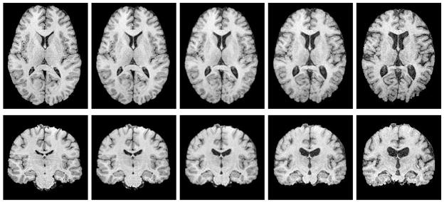
with boundary conditions I₀ = I and I₁ = I′. An example of a metamorphosis geodesic between two 3D MR brain images is shown in Figure 1. It was computed using a gradient descent on (5), which is described in further detail in Section 6.4.

Fig. 1.

Metamorphosis geodesic between two 3D brain images. Mid-axial (top row) and mid-coronal (bottom row) slices are shown.

2.2. Outliers, Robust Estimators And The Geometric Median

Outliers in data can throw off estimates of centrality based on the mean. One possible solution to this problem is outlier deletion, but removing outliers often merely promotes other data points to outlier status, forcing a large number of deletions before a reliable low-variance estimate can be found. The theory of robust estimators formalizes the idea that no individual point should affect measures of central tendency. The measure of robustness of an estimator is the breakdown point; formally, it is the fraction of the data that can be “dragged to infinity” (i.e., completely corrupted) without affecting the boundedness of the estimator. Clearly, the mean, whether it be a standard centroid or the more general Fréchet mean, has a breakdown point of 0, since as any single data point is dragged to infinity, the mean will grow without bound.

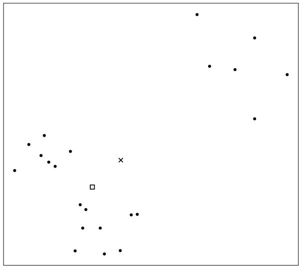
The theory of robust estimation has led to the development of numerous robust estimators, of which the L₁-estimator, also known as the geometric median, is one of the best known. Given a set of points {x_i, i = 1, ···, n} ∈ ℝ^d, with the usual Euclidean norm ||x||, the L₁-estimator is defined as the point m ∈ ℝ^d minimizing ${\sum }_{i=1}^n\parallel m-x_i\parallel$. It can be shown (Lopuhaä and Rousseeuw, 1991) that this estimator has a breakdown point of 0.5, which means that half of the data needs to be corrupted in order to corrupt this estimator. In Figure 2 we illustrate this by showing how the geometric median and the mean are displaced in the presence of a few outliers.

Fig. 2.

The geometric median (marked with a □) and mean (marked with a ×) for a collection of points in the plane. Notice how the few outliers at the top right of the picture have forced the mean away from the points, whereas the median remains centrally located.

The existence and uniqueness of the the median in ℝ^d follows directly from the convexity of the distance function. In one dimension, the geometric median is the point that divides the point set into equal halves on either side (if n is odd) and is any point on the line segment connecting the two middle points (if n is even). In general however, computing the geometric median is difficult; Bajaj has shown that the solution cannot be expressed using radicals (arithmetic operations, and k^th roots) (Bajaj, 1988).

There are two main approaches to computing the geometric median of a collection of points in ℝ^d. One way is to compute an approximate median m̃ such that ${\sum }_{i=1}^n\parallel \stackrel{\sim }{m}-x_i\parallel$ is at most a (1 + ε)-factor larger than cost of the optimal median. This can be computed using the ellipsoid method (Chandrasekaran and Tamir, 1990). A more efficient algorithm achieving the same result is due to Bose et al. (2003).

These algorithms do not generalize beyond Euclidean spaces. A more general iterative algorithm due to Weiszfeld (1937) and later improved by Kuhn and Kuenne (1962) and Ostresh (1978) converges to the optimal solution in Euclidean spaces (Kuhn, 1973), and was subsequently generalized to Banach spaces by Eckhardt (1980).

Several other robust estimators of centrality have been proposed in the statistics literature (Maronna et al., 2006). Winsorized means, where a percentage of extreme values are clamped, and trimmed means, where extreme values are removed, have been used for univariate data. The drawback of these methods is that they require a somewhat arbitrary selection of a threshold. M-estimators (Huber, 1981) are a generalization of maximum likelihood methods in which some function of the data is minimized. The geometric median is a special case of an M-estimator with an L¹ cost function.

3. The Riemannian Geometric Median

Let M be a Riemannian manifold. Given points x₁,…, x_n ∈ M and corresponding positive real weights w_i,…, w_n, with Σ_i w_i = 1, define the weighted sum-of-distances function f(x) = Σ_i w_id(x, x_i), where d is the Riemannian distance function on M. Throughout, we will assume that the x_i lie in a convex set U ⊂ M, i.e., any two points in U are connected by a unique shortest geodesic lying entirely in U. We define the weighted geometric median, m, as the minimizer of f, i.e.,

$$m=arg\underset{x\in M}{min}\sum _{i=1}^n{w}_{i}d(x,x_i).$$ (6)

When all the weights are equal, w_i = 1/n, we call m simply the geometric median.

In contrast, the Fréchet mean, or Karcher mean (Karcher, 1977), of a set of points on a Riemannian manifold is defined, via the generalization of the least squares principle in Euclidean spaces, as the minimizer of the sum-of-squared distances function,

$$\mu =arg\underset{x\in M}{min}\sum _{i=1}^n{w}_{i}d{(x,x_i)}^2.$$ (7)

We begin our exploration of the geometric median with a discussion of the Riemannian distance function. Given a point p ∈ M and a tangent vector v ∈ T_pM, where T_pM is the tangent space of M at p, there is a unique geodesic, γ: [0, 1] → M, starting at p with initial velocity v. The Riemannian exponential map, Exp_p : T_pM → M, maps the vector v to the endpoint of this geodesic, i.e., Exp_p(v) = γ(1). The exponential map is locally diffeomorphic onto a neighborhood of p. Let V (p) be the largest such neighborhood. Then within V (p) the exponential map has an inverse, the Riemannian log map, Log_p : V (p) → T_pM. For any point q ∈ V (p) the Riemannian distance function is given by d(p, q) = ||Log_p(q)||. For a fixed point p ∈ M, the gradient of the Riemannian distance function is ∇_xd(p, x) = −Log_x(p)/||Log_x(p)|| for x ∈ V (p). Notice that this is a unit vector at x, pointing away from p (compare to the Euclidean distance function).

The diameter of U, denoted diam(U), is the maximal distance between any two points in U. Using the convexity properties of the Riemannian distance function (see the Appendix for more details), we have the following existence and uniqueness result for the geometric median.

Theorem 1

The weighted geometric median defined by (6) exists and is unique if (a) the sectional curvatures of M are nonpositive, or if (b) the sectional curvatures of M are bounded above by Δ > 0 and $\text{diam}(U)<\pi /(2\sqrt{\mathrm{\Delta }})$.

Proof

Let γ : [a, b] → U be a geodesic. By the arguments in the Appendix, the distance function to any x_i is convex, that is, (d²/dt²)d(x_i, γ(t)) ≥ 0. Since the weighted sum-of-distances function f(x) is a convex combination of such functions, it is also convex. Furthermore, since the x_i do not all lie on the same geodesic, the vector Log_γ(t) (x_k) is not tangential to γ(t) for at least one k ∈ [1, n]. Therefore, by Lemma 1 we have (d²/dt²)d(x_k, γ(t)) > 0, and f (x) is a strictly convex function, which implies that the minimization (6) has a unique solution.

An isometry of a manifold M is a diffeomorphism f that preserves the Riemannian distance function, that is, d(x, y) = d(φ(x), φ(y)) for all x, y ∈ M. The set of all isometries forms a Lie group, called the isometry group. It is clear from the definition of the geometric median (6) that the geometric median is invariant under the isometry group of M. In other words, if m is the geometric median of {x_i} and φ is an isometry, then φ (m) is the geometric median of {φ(x_i)}. This is a property that the geometric median shares with the Fréchet mean.

4. The Breakdown Point of the Geometric Median

A standard measure of robustness for a centrality estimator in Euclidean space is the breakdown point, which is the minimal proportion of data that can be corrupted, i.e., made arbitrarily distant, before the statistic becomes unbounded. Let X = {x₁,…, x_n} be a set of points on M. Define the breakdown point of the geometric median as

$${\epsilon }^{\ast }(m,X)=\underset{1\le k\le n}{min}\left\{\frac{k}{n}:\underset{Y_k}{sup}d(m(X),m(Y_k))=\infty \right\},$$

where the supremum is taken over all sets Y_k that corrupt k points of X, that is, Y_k contains n − k points from the set X and k arbitrary points from M. Lopuhaä and Rousseeuw (1991) show that for the case M = ℝ^d the breakdown point is ε*(m, X) = ⌊(n +1)/2⌋/n. Notice that if M has bounded distance, then ε*(m, X) = 1. This is the case for compact manifolds such as spheres and rotation groups. Therefore, the breakdown point is only interesting in the case of manifolds with unbounded distance. The next theorem shows that the geometric median on unbounded manifolds has the same breakdown point as in the Euclidean case.

Theorem 2

Let U be a convex subset of M with diam(U) = ∞, and let X = {x₁,…, x_n} be a collection of points in U. Then the geometric median has breakdown point ε*(m, X) = ⌊ (n + 1)/2⌋/n.

Proof

The first part of the proof is a direct generalization of the argument for the Euclidean case given by (Lopuhaä and Rousseeuw, 1991) (Theorem 2.2). Let Y_k be a corrupted set of points that replaces k points from X, with k ≤ ⌊(n − 1)/2⌋. We show that for all such Y_k, d(m(X), m(Y_k)) is bounded by a constant. Let R = max_i d(m(X), x_i), and consider B = {p ∈ M: d(p, m(X)) ≤ 2R}, the ball of radius 2M about m(X). Let δ = inf_{p ∈ B} d(p, m(Y_k)). By the triangle inequality we have d(m(X), m(Y_k)) ≤ 2R + δ, and

$$\begin{array}{l}d(y_i,m(Y_k))\ge d(m(X),y_i)-d(m(X),m(Y_k))\\ \ge d(m(X),y_i)-(2R+\delta ).\end{array}$$

Now assume that δ > ⌊(n − 1)/2⌋2R. Then for the original points x_i we have

$$\begin{array}{l}d(x_i,m(Y_k))\ge R+\delta \\ \ge d(m(X),x_i)+\delta .\end{array}$$

Combining the two inequalities above with the fact that n−⌊(n − 1)/2⌋ of the y_i are from the original set X, we get

$$\begin{array}{l}\sum _{i=1}^{n}d(m(Y_k),y_i)\ge \sum _{i=1}^{n}d(m(X),y_i)-\lfloor (n-1)/2\rfloor (2R+\delta )\\ +(n-\lfloor (n-1)/2\rfloor )\delta \\ \ge \sum _{i=1}^{n}d(m(X),y_i)-\lfloor (n-1)/2\rfloor 2R+\delta \\ >\sum _{i=1}^{n}d(m(X),y_i).\end{array}$$

However, this is a contradiction since m(Y_k) minimizes the sum of distances, Σ_i d(m(Y_k), y_i). Therefore, d(m(Y_k), m(X)) ≤ 2R + δ ≤ ⌊ (n + 1)/2⌋2R. This implies that ε*(m, X) ≥ ⌊(n + 1)/2 ⌋/n.

The other inequality is proven with the following construction. Consider the case where k ≥ ⌊(n + 1)/2 ⌋ and each of the k corrupted points of Y_k are equal to some point p ∈ M. It is easy to show that m(Y_k) = p. Since we can choose the point p arbitrarily far away from m(X), it follows that ε*(m, X) ≥ ⌊(n + 1)/2⌋/n.

5. The Weiszfeld Algorithm for Manifolds

For Euclidean data the geometric median can be computed by an algorithm introduced by Weiszfeld (1937) and later improved by Kuhn and Kuenne (1962) and Ostresh (1978). The procedure iteratively updates the estimate m_k of the geometric median using essentially a steepest descent on the weighted sum-of-distances function, f. For a point x ∈ ℝⁿ not equal to any x_i, the gradient of f exists and is given by

$$\nabla f(x)=\sum _{i=1}^n{w}_i(x-x_i)/\parallel x-x_i\parallel .$$ (8)

The gradient of f(x) is not defined at the data points x = x_i. The iteration for computing the geometric median due to Ostresh is

$$\begin{array}{l}{m}_{k+1}=m_k-\alpha G_k,\\ G_k=\sum _{i\in I_k}\frac{w_i{x}_i}{\parallel x_i-m_k\parallel }·{\left(\sum _{i\in I_k}\frac{w_i}{\parallel x_i-m_k\parallel }\right)}^{-1},\end{array}$$ (9)

where I_k = {i ∈ [1, n] : m_k ≠ x_i}, and α > 0 is a step size. Notice if the current estimate m_k is located at a data point x_i, then this term is left out of the summation because the distance function is singular at that point. Ostresh (1978) proves that the iteration in (9) converges to the unique geometric median for 0 ≤ α ≤ 2 and when the points are not all colinear. This follows from the fact that f is strictly convex and (9) is a contraction, that is, f(m_k+1) < f (m_k) if m_k is not a fixed point.

Now for a general Riemannian manifold M, the gradient of the Riemannian sum-of-distances function is given by

$$\nabla f(x)=-\sum _{i=1}^n{w}_i{\text{Log}}_x(x_i)/d(x,x_i),$$ (10)

where again we require that x ∈ U is not one of the data points x_i. This leads to a natural steepest descent iteration to find the Riemannian geometric median, analogous to (9),

$$\begin{array}{l}{m}_{k+1}={\text{Exp}}_{m_k}(\alpha v_k),\\ v_k=\sum _{i\in I_k}\frac{w_i{\text{Log}}_{m_k}(x_i)}{d(m_k,x_i)}·{\left(\sum _{i\in I_k}\frac{w_i}{d(m_k,x_i)}\right)}^{-1}.\end{array}$$ (11)

The following result for positively curved manifolds shows that this procedure converges to the unique weighted geometric median when it exists.

Theorem 3

If the sectional curvatures of M are nonnegative and the conditions (b) of Theorem 1 are satisfied, then lim_{k → ∞} m_k = m for 0 ≤ α ≤ 2.

Proof

We use the fact that the Euclidean Weiszfeld iteration, given by (9), is a contraction. First, define f̃ (v) = Σ_i w_i||v − Log_mk(x_i)||, i.e., f̃ is the weighted sum-of-distances function for the log-mapped data, using distances in T_mk M induced by the Riemannian norm. Notice that the tangent vector v_k defined in (11) is exactly the same computation as the Euclidean Weiszfeld iteration (9), replacing each x_i with the tangent vector Log_mk (x_i). Therefore, we have the contraction property f̃ (α v_k) < f̃ (0). However, geodesics on positively curved manifolds converge, which means that distances between two points on the manifold are closer than their images under the log map. (This is a direct consequence of the Toponogov Comparison Theorem, see (Cheeger and Ebin, 1975)). In other words, d(Exp_mk (α v_k), x_i) < ||α v_k − Log_mk (x_i)||. This implies that f(m_k+1) = f (Exp_mk (αv_k)) < f̃ (α v_k) < f̃ (0) = f(m_k). (The last equality follows from ||Logm_k (x_i)|| = d(m_k, x_i).) Therefore, (11) is a contraction, which combined with f being strictly convex, proves that it converges to the unique solution m.

We believe that a similar convergence result will hold for negatively curved manifolds as well (with an appropriately chosen step size α). Since the algorithm is essentially a gradient descent on a convex function, there should be an α for which it converges, although in this case α may depend on the spread of the data. Our experiments presented in the next section for tensor data (Section 6.2) support our belief of convergence in this case. The tensor manifold has nonpositive curvature, and we found the procedure in (11) converged for α = 1. Proving convergence in this case is an area of future work.

6. Applications

In this section we present results of the Riemannian geometric median computation on 3D rotations, symmetric positive-definite tensors, planar shapes and, finally, the robust estimation of neuroanatomical atlases from brain images. For each example the geometric median is computed using the iteration presented in Section 5, which only requires computation of the Riemannian exponential and log maps. Therefore, the procedure is applicable to a wide class of manifolds beyond those presented here. The Fréchet mean is also computed for comparison using a gradient descent algorithm as described in (Fletcher et al., 2003) and elsewhere. It is important to note that unlike the Euclidean case where the mean can be computed in closed-form, both the Fréchet mean and geometric median computations for general manifolds are iterative, and we did not find any appreciable difference in the computation times in the examples described below.

6.1. Rotations

We represent 3D rotations as the unit quaternions, ℍ₁. A quaternion is denoted as q = (a, v), where a is the “real” component and v = bi + cj + dk. Geodesics in the rotation group are given simply by constant speed rotations about a fixed axis. Let e = (1, 0) be the identity quaternion. The tangent space T_eℍ₁ is the vector space of quaternions of the form (0, v). The tangent space at an arbitrary point q ∈ ℍ₁ is given by right multiplication of T_eℍ₁ by q. The Riemannian exponential map is Exp_q((0, v) · q) = (cos(θ/2), v · sin(θ/2)/θ) · q, where θ = ||v||. The log map is given by Log_q((a, v) · q) = (0, θ v/||v||) · q, where θ = 2 arccos(a).

To demonstrate the geometric median computations for 3D rotations, we generated a random collection of 20 quaternions. First, random tangent vectors were sampled from an isotropic Gaussian distribution with μ = 0, σ = π/30 in the tangent space at the identity. Next, the exponential map was applied to these random tangent vectors to produce random elements of ℍ₁, centered about the identity. The same procedure was repeated to generate sets of 5, 10, and 15 random outliers, whose mean now was rotated by 90 degrees from the original set. A sample of 8 of the original random rotations are displayed as 3D frames in the top row of Figure 3 along with 8 of the outliers in the bottom row.

Fig. 3.

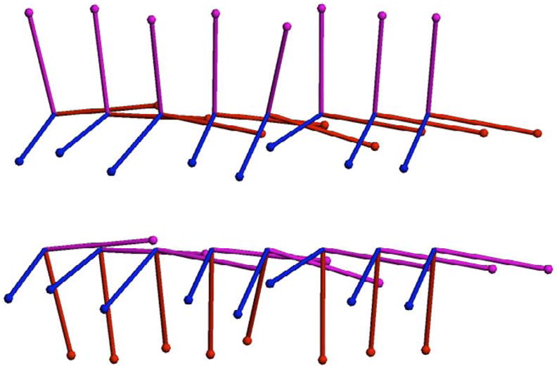
Eight rotations from the original dataset (top). Eight rotations from the outlier set (bottom).

We computed both the Fréchet mean and the geometric median of the original rotation dataset with 0, 5, 10, and 15 outliers included. This corresponds to an outlier percentage of 0%, 20%, 33%, and 43%, respectively. The geometric median was computed using the iteration in (11). The Fréchet mean was computed using the gradient descent algorithm described in (Buss and Fillmore, 2001). Both algorithms converged in under 10 iterations in a fraction of a second for all cases. The results are shown in Figure 4. The geometric median remains relatively stable even up to an addition of 15 outliers. In contrast, the Fréchet mean is dragged noticeably towards the outlier set.

Fig. 4.

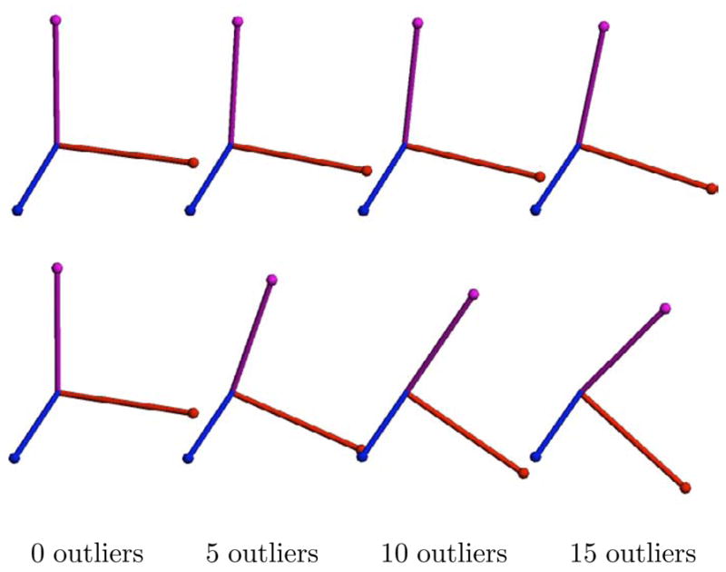
Comparison of the geometric median and Fréchet mean for 3D rotations. The geometric median results with 0, 5, 10, and 15 outliers (top). The Fréchet mean results for the same data (bottom).

6.2. Tensors

Positive definite symmetric matrices, or tensors, have a wide variety of uses in computer vision and image analysis, including texture analysis, optical flow, image segmentation, and neuroimage analysis. The space of positive definite symmetric tensors has a natural structure as a Riemannian manifold. Manifold techniques have successfully been used in a variety of applications involving tensors, which we briefly review now.

Diffusion tensor magnetic resonance imaging (DT-MRI) (Basser et al., 1994) gives clinicians the power to image in vivo the structure of white matter fibers in the brain. A 3D diffusion tensor models the covariance of the Brownian motion of water at a voxel, and as such is required to be a 3 × 3, symmetric, positive-definite matrix. Recent work (Batchelor et al., 2005; Fletcher and Joshi, 2004; Pennec et al., 2006; Wang and Vemuri, 2005) has focused on Riemannian methods for statistical analysis (Fréchet means and variability) and image processing of diffusion tensor data. The structure tensor (Bigun et al., 1991) is a measure of edge strength and orientation in images and has found use in texture analysis and optical flow. Recently, Rathi et al. (2007) have used the Riemannian structure of the tensor space for segmenting images. Finally, the Riemannian structure of tensor space has also found use in the analysis of structural differences in the brain, via tensor based morphometry (Lepore et al., 2006). Barmpoutis et al. (2007) describes a robust interpolation of DTI in the Riemannian framework by using a Gaussian weighting function to down-weight the influence of outliers. Unlike the geometric median, this method has the drawback of being dependent on the selection of the bandwidth for the weighting function.

We briefly review the differential geometry of tensor manifolds, which is covered in more detail in (Batchelor et al., 2005; Fletcher and Joshi, 2004; Pennec et al., 2006). Recall that a real n × n matrix A is symmetric if A = A^T and positive-definite if x^TAx > 0 for all nonzero x ∈ ℝⁿ. We denote the space of all n × n symmetric, positive-definite matrices as PD(n). Diffusion tensors are thus elements of PD(3), and structure tensors for 2D images are elements of PD(2). The tangent space of PD(n) at any point can be identified with the space of n × n symmetric matrices, Sym(n). Given a point p ∈PD(n) and a tangent vector X, the Riemannian exponential map is given by

$${\text{Exp}}_p(X)=p^{\frac{1}{2}}exp(\mathrm{\sum })p^{\frac{1}{2}T},\mathrm{\sum }=p^{-\frac{1}{2}}X{p}^{-\frac{1}{2}T},$$ (12)

where exp(Σ) is the matrix exponential and can be computed by exponentiating the eigenvalues of Σ, since it is symmetric. Likewise, the Riemannian log map between two points p, q ∈ PD(n) is given by

$${\text{Log}}_p(q)=p^{\frac{1}{2}}log(\mathrm{\Lambda })p^{\frac{1}{2}T},\mathrm{\Lambda }=p^{-\frac{1}{2}}q{p}^{-\frac{1}{2}T},$$ (13)

where log(Λ) is the matrix logarithm, computed by taking the log of the eigenvalues of Λ, which is well defined in the case of positive definite symmetric matrices.

As in the rotations example, we generated 20 random tensors as the image under the exponential map of Gaussian random tangent vectors. The mean was a tensor with eigenvalues λ₁ = 4 and λ₂ = λ₃ = 1. Next, sets of 5, 10, and 15 outliers were randomly generated in the same fashion with a mean tensor perpendicular to the original group. The standard deviation of both groups was σ = 0.2. A sample of 5 of the original tensor data and 5 of the outlier tensors are shown in Figure 5. The Fréchet mean and geometric median were computed for the tensor dataset including 0, 5, 10, and 15 outliers, and the results are shown in Figure 6. Again, convergence of the geometric median took less than 10 iterations in a fraction of a second. The tensors in Figures 5 & 6 are colored based on the orientation of the major eigenvector (green = original orientation, blue = outlier orientation) and with color modulated by the fractional anisotropy (Basser et al., 1994), i.e., more anisotropic tensors are more brightly colored. The geometric median retains the directionality and anisotropy of the original data, unlike the mean, which becomes more isotropic in the presence of outliers. This situation is common in DT-MRI, where adjacent white matter tracts may pass perpendicular to each other. In such cases, the geometric median would be a more appropriate local statistic than the mean to avoid contamination from tensors of a neighboring tract.

Fig. 5.

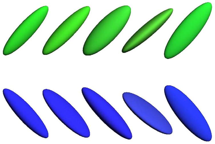
Five tensors from the original dataset (top). Five tensors from the outlier set (bottom).

Fig. 6.

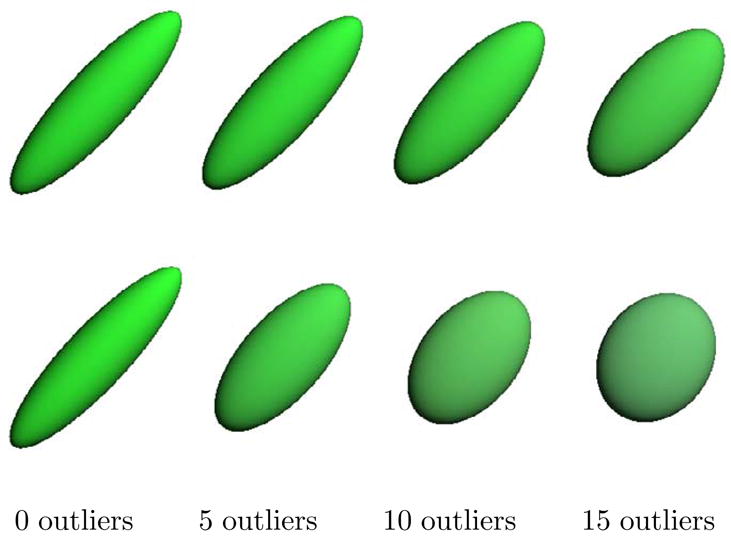
Comparison of the geometric median and Fréchet mean for 3D tensors. The geometric median results with 0, 5, 10, and 15 outliers (top). The Fréchet mean results for the same data (bottom).

6.3. Planar Shapes

One area of medical image analysis and computer vision that finds the most widespread use of Riemannian geometry is the analysis of shape. Dating back to the ground-breaking work of Kendall (1984) and Bookstein (1986), modern shape analysis is concerned with the geometry of objects that is invariant to rotation, translation, and scale. This typically results in representing an object’s shape as a point in a nonlinear Riemannian manifold, or shape space. Recently, there has been a great amount of interest in Riemannian shape analysis, and several shape spaces for 2D and 3D objects have been proposed (Fletcher et al., 2003; Grenander and Keenan, 1991; Klassen et al., 2004; Michor and Mumford, 2006; Sharon and Mumford, 2004; Younes, 1998).

An elementary tool in shape analysis is the computation of a mean shape, which is useful as a template, or representative of a population. The mean shape is important in image segmentation using deformable models (Cootes et al., 1995), shape clustering, and retrieval from shape databases (Srivastava et al., 2005). The mean shape is, however, susceptible to influence from outliers, which can be a concern for databases of shapes extracted from images. We now present an example showing the robustness of the geometric median on shape manifolds. We chose to use the Kendall shape space as an example, but the geometric median computation is applicable to other shape spaces as well.

We first provide some preliminary details of Kendall’s shape space (Kendall, 1984). A configuration of k points in the 2D plane is considered as a complex k-vector, z ∈ ℂ^k. Removing translation, by requiring the centroid to be zero, projects this point to the linear complex subspace V = {z ∈ ℂ^k: Σ z_i = 0}, which is equivalent to the space ℂ^k−1. Next, points in this subspace are deemed equivalent if they are a rotation and scaling of each other, which can be represented as multiplication by a complex number, ρe^iθ, where ρ is the scaling factor and θ is the rotation angle. The set of such equivalence classes forms the complex projective space, ℂP ^k−2. As Kendall points out, there is no unique way to identify a shape with a specific point in complex projective space. However, if we consider that the geometric median only require computation of exponential and log maps, we can compute these mappings relative to the base point, which requires no explicit identification of a shape with ℂP ^k−2.

Thus, we think of a centered shape x ∈ V as representing the complex line L_x = {z · x: z ∈ ℂ\{0}}, i.e., L_x consists of all point configurations with the same shape as x. A tangent vector at L_x ∈ V is a complex vector, v ∈V, such that 〈x, v〉 = 0. The exponential map is given by rotating (within V) the complex line L_x by the initial velocity v, that is,

$${\text{Exp}}_x(v)=cos\theta ·x+\frac{\parallel x\parallel sin\theta }{\theta }·v,\theta =\parallel v\parallel .$$ (14)

Likewise, the log map between two shapes x, y ∈V is given by finding the initial velocity of the rotation between the two complex lines L_x and L_y. Let π_x(y) = x · 〈x, y〉/||x||² denote the projection of the vector y onto x. Then the log map is given by

$${\text{Log}}_x(y)=\frac{\theta ·(y-{\pi }_x(y))}{\parallel y-{\pi }_x(y)\parallel },\theta =arccos\frac{\mid \langle x,y\rangle \mid }{\parallel x\parallel \parallel y\parallel }.$$ (15)

Notice that we never explicitly project a shape onto ℂP ^k−2. This has the effect that shapes computed via the exponential map (14) will have the same orientation and scale as the base point x. Also, tangent vectors computed via the log map (15) are valid only at the particular representation x (and not at a rotated or scaled version of x). This works nicely for our purposes and implies that the geometric median shape resulting from (11) will have the same orientation and scale as the intialization shape, m₀.

To test the robustness of the geometric median in Kendall shape space, we used the classic hand outlines from (Cootes et al., 1995). This data, shown in Figure 7, consists of 18 hand shapes, each with 72 points. We then generated a set of 12 ellipses as outliers. Each ellipse was generated as (a cos(θ_k), b sin(θ_k), where a, b are two uniformly random numbers in [0.5, 1] and θ_k = kπ/36, k = 0, …, 71. We computed the Fréchet mean and geometric median for the hand data with 0, 2, 6, and 12 outliers included, corresponding to 0%, 10%, 25%, and 40% outliers, respectively. Both the mean and geometric median computations converge in under 15 iterations, running in less than a second for each of the cases. The results are shown in Figure 9. With enough outliers the Fréchet mean is unrecognizable as a hand, while the geometric median is very stable even with 40% outliers. To ensure that both the Fréchet mean and the geometric median computations were not caught in local minima, we initialized both algorithms with several different data points, including several of the outlier shapes. In each case the Fréchet mean and geometric median converged to the same results as shown in Figure 9.

Fig. 7.

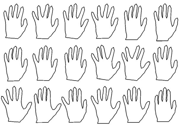
The original dataset of 18 hand shapes.

Fig. 9.

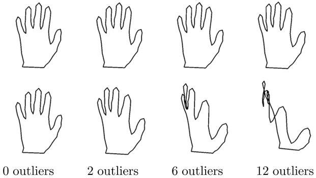
The gometric median shape (top row) from the hand database with 0, 2, 6, and 12 outliers included. The Fréchet mean shape (bottom row) using the same data.

6.4. Deformable Images

We now present the application of the manifold geometric median algorithm developed above for robust atlas estimation from a collection of grayscale images. To do this in a fashion that combines geometric variability as well as intensity changes in the images, we use the metamorphosis metric reviewed in Section 2.1. The algorithms to compute the Fréchet mean and the geometric median of a set of images Iⁱ, i = 1, …, n are slightly different than in the above finite-dimensional examples. Rather than computing exponential and log maps for the metamorphosis metric, we compute a gradient descent on the entire energy functional and optimize the atlas image simultaneously with the geodesic paths. We begin with a description of the computation for the Fréchet mean image, μ. We now have n metamorphoses ( $f_t^i,g_t^i$), where $I^i(t)=g_t^i·f_t^i$ has boundary conditions $I_0^i=\mu$ and $I_1^i=I^i$. In other words, each path starts at the atlas image μ and ends at an input image. The Fréchet mean is computed by minimizing the sum of geodesic energies, i.e.,

$$\mu ={arg}_I\underset{I,v^i}{min}\sum _{i=1}^{n}U(v_t^i,I_t^i),\text{subject}\text{to}{I}_0^i=I,I_1^i=I^i.$$ (16)

Similarly, the geometric median image, m, is computed by minimizing the sum of square root geodesic energies, i.e.,

$$m={arg}_I\underset{I,v^i}{min}\sum _{i=1}^n\sqrt{U(v_t^i,I_t^i)},\text{subject}\text{to}{I}_0^i=I,I_1^i=I^i.$$ (17)

Following Garcin and Younes (2005), we compute geodesics directly using the discretized version of the energy functional U. Denoting a discretized metamorphosis by I_t, t = 1 …, T, and v_t, t = 1, …, T − 1, the energy of this path is given by

$$U(I,v)=\sum _{t=1}^{T-1}\langle L{v}_t,v_t\rangle +\frac{1}{{\sigma }^2}\parallel {\mathcal{T}}_{v_t}{I}_{t+1}-I_t\mid {\mid }^2,$$ (18)

where T_vI denotes trilinear interpolation of the transformed image I(x + v(x)). The gradients of U with respect to both v and I are given by

$$\begin{array}{l}{\nabla }_{v_t}U(I,v)=v_t-\frac{1}{{\sigma }^2}K[({\mathcal{T}}_{v_t}{I}_{t+1}-I_t){\mathcal{T}}_{v_t}\nabla I_{t+1}],\\ {\sigma }^2{\nabla }_{I_t}U(I,v)=I_t-{\mathcal{T}}_{v_t}{I}_{t+1}+{\mathcal{T}}_{v_t}^T(T_{v_{t-1}}{I}_t-I_{t-1}),\end{array}$$

where ${\mathcal{T}}_v^T$ denotes the adjoint of the trilinear interpolation operator (see (Garcin and Younes, 2005) for details), and K = L⁻¹. Finally, given a discretized version of the Fréchet mean equation (16) and discretized paths $I_t^i,v_t^i,i=1,\dots ,n$, we denote the total sum-of-square geodesic energies by

$$E_{\mu }(I^i,v^i)=\sum _{i=1}^{n}U(I^i,v^i),\text{such}\text{that}{I}_1^i=\mu .$$

The gradient of E_μ with respect to the Fréchet mean atlas, μ, is

$${\nabla }_{\mu }{E}_{\mu }(I^i,v^i)=\frac{1}{{\sigma }^2}\sum _{i=1}^n\left(\mu -{\mathcal{T}}_{v_1^i}{I}_2^i\right).$$

For computing the geometric median from the discretized version of (17), the gradients for the individual paths are given by

$$\begin{array}{l}{\nabla }_{v_t}\sqrt{U(I,v)}={\nabla }_{v_t}U(I,v)/2\sqrt{U(I,v)},\\ {\nabla }_{I_t}\sqrt{U(I,v)}={\nabla }_{I_t}U(I,v)/2\sqrt{U(I,v)}.\end{array}$$

We denote the total discretized energy functional for the geometric median by

$$E_m(I^i,v^i)=\sum _{i=1}^n\sqrt{U(I^i,v^i)},\text{such}\text{that}{I}_1^i=m.$$

Now, the gradient of E_m with respect to the geometric median atlas, m, has the form

$${\nabla }_m{E}_m(I^i,v^i)=\sum _{i=1}^n(m-{\mathcal{T}}_{v_1^i}{I}_2^i)/\sqrt{\langle L{v}_1,v_1\rangle +\frac{1}{{\sigma }^2}\parallel {\mathcal{T}}_{v_1^i}{I}_2^i-m\mid {\mid }^2}$$

We first tested the geometric median atlas estimation using synthesized 3D bullseye images, consisting of concetric spheres with different grayscales. We created three spherical bullseye images with varying radii. We then added a single outlier image that was a bullseye with anisotropic aspect ratio. Slices from the input images are shown in Figure 10. Finally, we computed the geometric median and Fréchet mean atlases under the metamorphosis metric as described in this section (Figure 11). The Fréchet mean atlas is geometrically more similar to the outlier, i.e., it has an obvious oblong shape. However, the geometric median atlas is able to better retain the spherical shape of the original bullseye data.

Fig. 10.

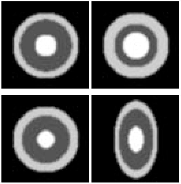
2D cross-sections from the input images for the 3D bullseye example. The bottom right image is an outlier.

Fig. 11.

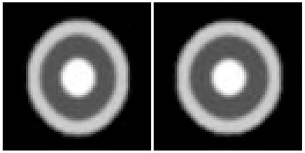
The Fréchet mean of the bullseye images (left) and the geometric median (right), both using the metamorphosis metric. Notice the mean is affected more by the outlier, while the median retains the spherical shape of the main data.

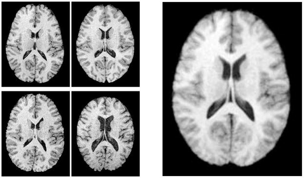
Finally, we tested the geometric median atlas estimation from a set of 3D MR brain images. The input images were chosen from a database containing MRA, T1-FLASH, T1-MPRAGE, and T2-weighted images from 97 healthy adults ranging in age from 20 to 79 (Lorenzen et al., 2006). For this study we only utilized the T1-FLASH images. These images were acquired at a spatial resolution of 1mm×1mm×1mm using a 3 Tesla head-only scanner. The tissue exterior to the brain was removed using a mask generated by a brain segmentation tool described in (Prastawa et al., 2004). This tool was also used for bias correction. In the final preprocessing step, all of the images were spatially aligned to an atlas using affine registration. We applied our geometric median atlas estimation to a set of four MR images from the database. The resulting atlas is shown on the right side of Figure 12. In this case the geometric median atlas was nearly identical to the Fréchet mean atlas, most likely because there is no clear outlier in the MR images. We expect the median atlas construction to be useful in cases where there are gross anatomical outliers.

Fig. 12.

Midaxial slices from the four input 3D MR images (left). The resulting geometric median atlas (right).

7. Conclusion and Discussion

In this paper we extended the notion of the geometric median, a robust estimator of centrality, to manifold-valued data. We proved that the geometric median exists and is unique for any non positively curved manifold and under certain conditions for positively curved manifolds. Generalizing the Weiszfeld algorithm, we introduced a procedure to find the Riemannian geometric median and proved that it converged on positively curved manifolds. Applications to the 3D rotation group, tensor manifolds, and planar shape spaces were presented with comparisons to the Fréchet mean.

We expect the geometric median to be useful in several image analysis applications. For instance, the geometric median could be used to robustly train deformable shape models for image segmentation applications. In this application and in robust atlas construction we believe the geometric median will have advantages to the Fréchet mean when the data includes anatomical outliers due to misdiagnosis, segmentation errors, or anatomical abnormalities. In diffusion tensor imaging we envision the geometric median being used as a median filter or for robust tensor splines (similar to (Barmpoutis et al., 2007)). This would preserve edges in the data at the interface of adjacent tracts. The geometric median could also be used for along-tract summary statistics for robust group comparisons (along the lines of Corouge et al. (2006); Fletcher et al. (2007); Goodlett et al. (2008)).

Since the area of robust estimation on manifolds is largely unexplored, there are several exciting opportunities for future work. Least squares estimators of the spread of the data have been extended to manifolds via tangent space covariances (Pennec, 2006) and principal geodesic analysis (PGA) (Fletcher et al., 2003). Noting that the median is an example of an L¹ M-estimator, the techniques presented in this paper can be applied to extend notions of robust covariances and robust PCA to manifold-valued data. Other possible applications of the Riemannian geometric median include robust clustering on manifolds, filtering and segmentation of manifold-valued images (e.g., images of tensor or directional data).

Fig. 8.

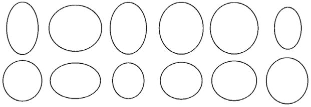
The 12 outlier shapes.

8. Appendix

Here we outline the convexity properties of the Riemannian distance function. Our argument follows along the same lines as Karcher (1977), who proves the convexity of the squared distance function. Let U be a convex subset of a manifold M. Let γ: [a, b] → U be a geodesic and consider the variation of geodesics from p ∈ U to γ given by c(s, t) = Exp_p(s ··Log_p(γ(t))). To prove convexity of the Riemannian distance function, we must show that the second derivative $\frac{d^2}{d{t}^2}d(p,\gamma (t))$ is strictly positive. Denote c′ = (d/ds)c(s, t) and ċ = (d/dt)c(s, t). (Readers familiar with Jacobi fields will recognize that ċ is a family of Jacobi fields.) The second derivative of the distance function is given by

$$\begin{array}{l}\frac{d^2}{d{t}^2}d(p,\gamma (t))=\\ \frac{\langle \stackrel{.}{c}(1,t),(D/ds)\stackrel{.}{c}(1,t)\rangle }{d(p,\gamma (t))}-\frac{{\langle \stackrel{.}{c}(1,t),c^{\prime }(1,t)\rangle }^2}{d{(p,\gamma (t))}^3}.\end{array}$$ (19)

When ċ(1, t) is tangential to γ(t), i.e., γ is a geodesic towards (or away from) p, we can easily see that $\frac{d^2}{d{t}^2}d(p,\gamma (t))=0$. Now let ċ^⊥(1, t) be the component of ċ(1, t) that is normal to γ(t). We use the following result from (Karcher, 1977).

Lemma 1

If the sectional curvature of M is bounded above by Δ > 0 and $\text{diam}(U)<\pi /(2\sqrt{\mathrm{\Delta }})$, then 〈ċ^⊥(1, t), (D/ds)c′(1, t)〉 > 0. If M has nonpositive curvature (Δ ≤ 0), then the result holds with no restriction on the diameter of U.

Along with 〈ċ^⊥(1, t), c′(1, t)〉 = 0, Lemma 1 implies that $\frac{d^2}{d{t}^2}d(p,\gamma (t))$ is strictly positive when Log_{γ (t)}(p) is not tangential to γ(t).

References

- Bajaj C. The algebraic degree of geometric optimization problems. Discrete and Computational Geometry. 1988;3:177–191. [Google Scholar]
- Barmpoutis A, Vemuri BC, Shepherd TM, Forder JR. Tensor splines for interpolation and approximation of DT-MRI with application to segmentation of isolated rat hippocampi. IEEE Transactions on Medical Imaging. 2007;26 (11):1537–1546. doi: 10.1109/TMI.2007.903195. [DOI] [PMC free article] [PubMed] [Google Scholar]
- Basser PJ, Mattiello J, Bihan DL. MR diffusion tensor spectroscopy and imaging. Biophysics Journal. 1994;66:259–267. doi: 10.1016/S0006-3495(94)80775-1. [DOI] [PMC free article] [PubMed] [Google Scholar]
- Batchelor P, Moakher M, Atkinson D, Calamante F, Connelly A. A rigorous framework for diffusion tensor calculus. Magnetic Resonance in Medicine. 2005;53:221–225. doi: 10.1002/mrm.20334. [DOI] [PubMed] [Google Scholar]
- Bigun J, Granlund G, Wiklund J. Multidimensional orientation estimation with application to texture analysis and optical flow. IEEE Transactions on Pattern Analysis and Machine Intelligence. 1991;13 (8):775–790. [Google Scholar]
- Bookstein FL. Size and shape spaces for landmark data in two dimensions (with discussion) Statistical Science. 1986;1 (2):181–242. [Google Scholar]
- Bose P, Maheshwari A, Morin P. Fast approximations for sums of distances, clustering and the fermat–weber problem. Comput Geom Theory Appl. 2003;24(3):135–146. [Google Scholar]
- Buss SR, Fillmore JP. Spherical averages and applications to spherical splines and interpolation. ACM Transactions on Graphics. 2001;20 (2):95–126. [Google Scholar]
- Chandrasekaran R, Tamir A. Algebraic optimization: The Fermat-Weber problem. Mathematical Programming. 1990;46:219–224. [Google Scholar]
- Cheeger J, Ebin DG. Comparison Theorems in Riemannian Geometry. North-Holland: 1975. [Google Scholar]
- Cootes TF, Taylor CJ, Cooper DH, Graham J. Active shape models – their training and application. Comp Vision and Image Understanding. 1995;61 (1):38–59. [Google Scholar]
- Corouge I, Fletcher PT, Joshi S, Gouttard S, Gerig G. Fiber tract-oriented statistics for quantitative diffusion tensor MRI analysis. Medical Image Analysis. 2006;10 (5):786–798. doi: 10.1016/j.media.2006.07.003. [DOI] [PubMed] [Google Scholar]
- Eckhardt U. Weber’s problem and Weiszfeld’s algorithm in general spaces. Mathematical Programming. 1980;18:186–196. [Google Scholar]
- Fletcher PT, Joshi S. Principal geodesic analysis on symmetric spaces: statistics of diffusion tensors. Proceedings of ECCV Workshop on Computer Vision Approaches to Medical Image Analysis; 2004. pp. 87–98. [Google Scholar]
- Fletcher PT, Lu C, Joshi S. Statistics of shape via principal geodesic analysis on Lie groups. Proceedings of the IEEE Conference on Computer Vision and Pattern Recognition; 2003. pp. 95–101. [Google Scholar]
- Fletcher PT, Tao R, Jeong WK, Whitaker RT. A volumetric approach to quantifying region-to-region white matter connectivity in diffusion tensor MRI. Proceedings of Information Processing in Medical Imaging (IPMI); 2007. pp. 346–358. [DOI] [PubMed] [Google Scholar]
- Fréchet M. Les éléments aléatoires de nature quel-conque dans un espace distancié. Ann Inst H Poincaré. 1948;10 (3):215–310. [Google Scholar]
- Garcin L, Younes L. Geodesic image matching: a wavelet based energy minimization scheme. Workshop on Energy Minimization Methods in Computer Vision and Pattern Recognition (EMMCVPR); 2005. pp. 349–364. [Google Scholar]
- Goodlett C, Fletcher PT, Gilmore J, Gerig G. Group statistics of DTI fiber bundles using spatial functions of tensor measures. Proceedings of Medical Image Computing and Computer Assisted Intervention (MICCAI); 2008. pp. 1068–1075. [DOI] [PMC free article] [PubMed] [Google Scholar]
- Grenander U, Keenan DM. On the shape of plane images. SIAM J Appl Math. 1991;53:1072–1094. [Google Scholar]
- Huber PJ. Robust Statistics. John Wiley; New York.: 1981. [Google Scholar]
- Joshi S, Davis B, Jomier M, Gerig G. Unbiased diffeomorphic atlas construction for computational anatomy. Neuroimage. 2004;23(Suppl 1):S151–160. doi: 10.1016/j.neuroimage.2004.07.068. [DOI] [PubMed] [Google Scholar]
- Karcher H. Riemannian center of mass and mollifier smoothing. Comm on Pure and Appl Math. 1977;30:509–541. [Google Scholar]
- Kendall DG. Shape manifolds, Procrustean metrics, and complex projective spaces. Bulletin of the London Mathematical Society. 1984;16:18–121. [Google Scholar]
- Klassen E, Srivastava A, Mio W, Joshi S. Analysis of planar shapes using geodesic paths on shape spaces. IEEE Transactions on Pattern Analysis and Machine Intelligence. 2004;26 (3):372–383. doi: 10.1109/TPAMI.2004.1262333. [DOI] [PubMed] [Google Scholar]
- Kuhn HW. A note on Fermat’s problem. Mathematical Programming. 1973;4:98–107. [Google Scholar]
- Kuhn HW, Kuenne RE. An efficient algorithm for the numerical solution of the generalized Weber problem in spatial economics. J Regional Sci. 1962;4:21–34. [Google Scholar]
- Lepore N, Brun CA, Chiang M-C, Chou Y-Y, Dutton RA, Hayashi KM, Lopez OL, Aizenstein HJ, Toga AW, Becker JT, Thompson P. Multivariate statistics of the Jacobian matrices in tensor based morphometry and their application to HIV/AIDS. MICCAI. 2006:191–198. doi: 10.1007/11866565_24. [DOI] [PubMed] [Google Scholar]
- Lopuhaä HP, Rousseeuw PJ. Breakdown points of affine equivariant estimators of multivariate location and covariance matrices. The Annals of Statistics. 1991;19 (1):229–248. [Google Scholar]
- Lorenzen P, Prastawa M, Davis B, Gerig G, Bullitt E, Joshi S. Multi-modal image set registration and atlas formation. Medical Image Analysis. 2006;10 (3):440–451. doi: 10.1016/j.media.2005.03.002. [DOI] [PMC free article] [PubMed] [Google Scholar]
- Maronna RA, Martin DR, Yohai VJ. Robust Statistics: Theory and Methods. John Wiley; West Sussex, England.: 2006. [Google Scholar]
- Michor PW, Mumford D. Riemannian geometries on spaces of plane curves. J Eur Math Soc. 2006;8:1–48. [Google Scholar]
- Miller M, Younes L. Group actions, homeomorphisms, and matching: a general framework. International Journal of Computer Vision. 2001;41 (1–2):61–84. [Google Scholar]
- Ostresh LM. On the convergence of a class of iterative methods for solving the Weber location problem. Operations Research. 1978;26:597–609. [Google Scholar]
- Pennec X. Intrinsic statistics on Riemannian manifolds: basic tools for geometric measurements. Journal of Mathematical Imaging and Vision. 2006;25(1) [Google Scholar]
- Pennec X, Fillard P, Ayache N. A Riemannian framework for tensor computing. International Journal of Computer Vision. 2006;61 (1):41–66. [Google Scholar]
- Prastawa M, Bullitt E, Ho S, Gerig G. A brain tumor segmentation framework based on outlier detection. Medical Image Analysis. 2004;8 (3):275–283. doi: 10.1016/j.media.2004.06.007. [DOI] [PubMed] [Google Scholar]
- Rathi Y, Tannenbaum A, Michailovich O. Segmenting images on the tensor manifold. IEEE Conference on Computer Vision and Pattern Recognition; 2007. pp. 1–8. [Google Scholar]
- Sharon E, Mumford D. 2d-shape analysis using conformal mapping. Proceedings of the IEEE Conference on Computer Vision and Pattern Recognition; 2004. pp. 350–357. [Google Scholar]
- Srivastava A, Joshi S, Mio W, Liu X. Statistical shape analysis: clustering, learning, and testing. IEEE Transactions on Pattern Analysis and Machine Intelligence. 2005;27 (4):590–602. doi: 10.1109/TPAMI.2005.86. [DOI] [PubMed] [Google Scholar]
- Trouvé A, Younes L. Metamorphoses through Lie group action. Foundations of Computational Mathematics. 2005;5(2) [Google Scholar]
- Wang Z, Vemuri BC. DTI segmentation using an information theoretic tensor dissimilarity measure. IEEE Transactions on Medical Imaging. 2005;24 (10):1267–1277. doi: 10.1109/TMI.2005.854516. [DOI] [PubMed] [Google Scholar]
- Weiszfeld E. Sur le point pour lequel la somme des distances de n points donnés est minimum. Tohoku Math J. 1937;43:355–386. [Google Scholar]
- Younes L. Computable elastic distances between shapes. SIAM J Appl Math. 1998;58:565–586. [Google Scholar]