Analysis of facial motion patterns during speech using a matrix factorization algorithm

Abstract

This paper presents an analysis of facial motion during speech to identify linearly independent kinematic regions. The data consists of three-dimensional displacement records of a set of markers located on a subject’s face while producing speech. A QR factorization with column pivoting algorithm selects a subset of markers with independent motion patterns. The subset is used as a basis to fit the motion of the other facial markers, which determines facial regions of influence of each of the linearly independent markers. Those regions constitute kinematic “eigenregions” whose combined motion produces the total motion of the face. Facial animations may be generated by driving the independent markers with collected displacement records.

INTRODUCTION

The general goal of this work is to develop a mathematical model of facial biomechanics for applications to speech production and perception studies. The model must be capable of producing computer-generated animations of speech with an acceptable level of realism and should allow for direct manipulation of facial movement parameters (Munhall and Vatikiotis Bateson, 1998).

The core of such a system must be some mathematical representation of the physiology of the human face. When building models of facial physiology, two general strategies have been followed (cf. Beautemps et al., 2001). One is a theoretical modeling strategy, in which the physiological structure of passive tissues and active muscles is explicitly described commonly by differential equations. The face behavior is simulated by computing the forces that act on the tissues and their resultant deformations. In this way, the dynamics of the system is incorporated into the model. Such models are theoretical in the sense that assumptions are made in choosing the key attributes of the models and parameters are estimated or determined from best available measures from the literature. This strategy was pioneered by the muscle-based facial animation work of Terzopoulos and Waters (1990); Lee et al., (1995); and Parke and Waters (1996), in which some of the facial muscles and some aspects of the soft tissue were modeled. Following their work, a three-dimensional (3D) biomechanical model of the face was developed for producing animations of speech (Lucero and Munhall, 1999). The model was driven by recorded perioral electromyographic signals and, in a later version, by records of facial kinematics (Pitermann and Munhall, 2001). In general, the model was able to generate animations with a reasonable level of visual realism and showed potential as a computational tool to study the facial physiology of speech. However, it has been argued that, in its current stage of development, the strategy is still not appropriate for the intended application to speech perception research (Lucero et al., 2005). Its main drawback is the difficulty of producing a representation of the complex structure of muscles and passive tissues precise enough to capture details of speech movement patterns and, at the same time, that could be easily adapted to different subjects.

Within this general strategy, the application of free form deformations by Kalra et al. (1992) may also be included. There each facial muscle is represented as a deformable facial region, whose motion is controlled by the movement of a facial point. The geometry of the facial regions and their deformation properties are defined based on information from available anatomical data. Although the result is not a dynamical model, it is still a theoretical representation of the face (because it is based on average physical and anatomical parameters and it thus represents a generic face), and suffers from the same drawbacks noted above.

A second strategy is empirical modeling. In this case, a relation between various facial parameters measured during speech is constructed. For example, in Kuratate et al.’s statistical modeling work (Kuratate et al., 1998), principal component analysis (PCA) is used to decompose a set of measured facial shapes into orthogonal components, and determine a reduced base of eigenfaces. Arbitrary facial shapes and movements are next generated by driving a linear combination of the eigenfaces. The physiology of the face is not modeled explicitly, although it is still present, in implicit form, in the model’s equations. Besides facial kinematics, other speech parameters may be incorporated into the model, such as muscle electromyography and acoustics (Vatikiotis-Bateson and Yehia, 1996; Kuratate et al., 1999). Similar empirical modeling strategies using independent component analysis (ICA) have also been proposed (Müller et al., 2005).

In a previous work (Lucero et al., 2005), an empirical model was introduced that was based on decomposing the face surface into a finite set of regions. The total motion of the face was computed as the linear combination of the movement of those regions. The model was built by analyzing the recorded 3D position of a set of markers placed on a subject’s face, while producing a sequence of sentences. An algorithm grouped the markers into a set of clusters, which had one primary marker and a number of secondary markers with associated weights. The displacement of each secondary marker was next expressed as the linear combination of the displacements of the primary markers of the clusters to which it belonged. The model was next used to generate facial animations, by driving the primary markers and associated clusters with collected data.

It was argued that the computed cluster structure represented the degrees of freedom (DOF) of the system. The DOF are the independent modes of variation and thus the independent sources of information. Subjects differ in the information transmission from their faces and this may be due in part to differences in their DOF. In the model, the facial clusters define facial eigenregions, whose combined motion forms the total motion of the facial surface.

This empirical model and the PCA (or ICA) approach are based on linear modeling of the data which can result in similar levels of accuracy in reconstruction of the data. However, the resulting solutions are quite different and serve different purposes. The PCA approach extracts global structure and will produce a set of primary gestures. Its DOF are the functional modes of deformation of the face. In the present case, the aim is to identify a set of spatially distinct regions that move independently as the DOF. There presumably is a mapping between these two representations and it could be hypothesized that the nervous system must know what to control in its anatomical DOF to produce its gestural basis set.

There are a number of advantages to focusing on the spatial DOF. This approach focuses the data analysis on the generating mechanism for gestures: The facial musculature. The action of muscles is obviously spatially concentrated and thus facial regions can be found that are associated with individual muscles or synergies of muscles that are in close proximity or whose actions are spatially localized. This muscle-based approach is consistent with a productive tradition in the analysis of facial expression and the study of perception of expressions (Ekman et al., 2002) and this approach has also been a powerful tool in facial animation (e.g., Terzopoulos and Waters, 1990). Another advantage of finding regional DOF in a data set is that these regions can be animated in arbitrary facial configurations. There is considerable interest in speech perception research on the role of individual talker characteristics in speech perception (e.g., Goldinger, 1996). Studies that involve the use of animating a generic face or the animation of one talkers morphology with another talkers motion must solve a registration and morphing problem (Knappmeyer et al., 2003). The identification of key features and spatial regions is one form of solution to this correspondence problem.

This empirical modeling approach is close to the articulatory modeling work of Badin, Bailly, et al. (Badin et al., 2002; Beautemps et al., 2001; Engwall and Beskow, 2003). In their work, PCA is used to determine articulatory parameters to control the shape of a 3D vocal tract and face model. For better correspondence to the underlying biomechanics, some of the parameters (e.g., jaw height, lip protrusion, etc.) are defined a priori, and their contributions are subtracted from the data before computing the remaining components. The present approach proposes to rely entirely on the data to build the model, with as few prior assumptions as possible. Instead of setting a model by defining the biomechanical properties of skin tissue and muscle structure based on a priori theoretical reasons, a possible model is inferred just by looking at the measured motion patterns of the facial surface.

The algorithm presented by Lucero et al. (2005) had a preliminary nature and had some drawbacks. For example, it was necessary to define an initial facial mesh, linking nodes corresponding to the initial position of the markers and leaving “holes” for the eyes and mouth. Also, a more solid foundation for the criteria for grouping the markers was desired. In the present paper, an improved version is introduced, which uses a QR factorization technique (Golub and Loan, 1996) to identify a linearly independent subset of facial markers. This subset is next used as a basis to predict the displacement of arbitrary facial points.

DATA

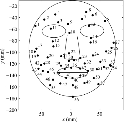
The data consist of the 3D position of 57 markers distributed on a subject’s face, recorded with a Vicon equipment (Vicon Motion Systems, Inc., Lake Forest, CA) at a 120 Hz sampling frequency. According to calibration data, the position measures were accurate within 0.5 mm. An additional six markers on a head band were used to determine a head coordinate system, with the positive directions of its axes defined as: the x axis in the horizontal direction from right to left, the y axis in the vertical direction to the top, and the z axis in the protrusion direction to the front. The position of the 57 facial markers was expressed in those coordinates, with the approximate location shown in Fig. 1. Neither the morphology of subjects’ faces nor the precise placement of the markers is exactly symmetrical and thus the markers seem to be offset from the facial features in the schematic and symmetrical face in the figure.

Figure 1.

Spatial distribution of the marker positions superimposed on a schematic face.

Data were recorded from 2 subjects (S1 and S2), while they were producing selected sentences from the Central Institute for the Deaf Everyday sentences (Davis and Silverman, 1970), listed in http:∕∕www.mat.unb.br∕lucero∕facial∕qr2.html. A large portion of the data for the marker at the left upper eyelid (marker 13) of subject S1 was missing, due to recording errors. Since the motion patterns of right and left upper eyelids seemed very close (by visual assessment), the missing data of the left upper eyelid were copied from the marker at the other eyelid. It will be shown later that the algorithm detected this artifact within the data, which serves as a proof of its ability to analyze kinematic patterns.

A total of 40 sentences was recorded from subject S1 and 50 sentences from subject S2. In the case of S2, the set of 50 sentences was recorded twice, forming two datasets which will be denoted as S2a and S2b. In the recording sessions, the subjects were asked to adopt a consistent rest position at the beginning of each sentence. The initial positions of the markers were taken as representative of a rest (neutral) configuration.

THE SUBSET SELECTION PROBLEM

This approach for building an empirical facial model is based on the so-called subset selection problem of linear algebra (Golub and Loan, 1996). Assume a given data matrix A∊R^m×n and the observation vector b∊R^m×1, with m⩾n, and that a predictor vector x is sought in the least squares sense, which minimizes ${\Vert Ax-b\Vert }_2^2$. Assume also that the data matrix A derives from observations of redundant factors. Therefore, instead of using the whole data matrix A to predict b, it may be desirable to use only a subset of its columns, so as to filter out the data redundancy. The problem is, then, how to pick the nonredundant columns. In the present case of facial modeling, the data matrix will contain the displacements of the 57 facial markers, arranged in columns. A small subset of markers (columns of the data matrix) must be selected which may be used to predict the motion of any other arbitrary facial point.

The idea of reducing the data set is consistent with the long-held view that the speech production system is itself low-dimensional. As Bernstein (1967) suggested about motor control in general, the nervous system acts to reduce the potential DOF. In speech the muscles and articulators are coupled synergistically during articulation in order to produce particular sounds.

To solve the subset selection problem, the most linearly independent columns of matrix A must be identified. Let A_k denote a subset of k columns of A. A measure of “independency” of the subset is provided by the smallest singular value of A_k, σ_k, which measures the distance of A_k to the set of k-rank singular matrices, in the 2-norm. Thus, it indicates how far A_k is from being a singular matrix. Consequently, the smaller σ_k, the more independent the subset A_k. In principle, the subset selection problem could be solved by testing all possible combinations of k columns from the total of n columns of A. The number of possible combinations is n!∕[k!(n−k)!], which could be prohibitively large. In the present case, with n=57 and adopting k=10 as an example, the number of combinations is 4.32×10¹⁰. So far, it appears that an exhaustive search is the only means to compute the optimal solution to the problem (Lawson and Hanson, 1987; Björck, 2004).

A possible solution to the subset selection problem is provided by the algorithm of QR factorization with column pivoting (Golub and Loan, 1996; Chan and Hansen, 1992). That algorithm decomposes A in the form AΠ=QR, where Π∊R^n×n is a column permutation matrix, Q∊R^m×n is an orthogonal matrix, and R∊R^n×n is an upper triangular matrix with positive diagonal elements1 The first column of the permutated matrix AΠ is just the column of A that has the largest 2-norm (euclidean norm). The second column of AΠ is the column of A that has the largest component in a direction orthogonal to the direction of first column. In general, the kth column of AΠ is the column of A with the largest component in a direction orthogonal to the directions of first k−1 columns [or, equivalently, is the column of A which has maximum distance from the subspace spanned by the first k−1 columns (Björck, 2004)]. The diagonal elements of R (r_kk), also called the R values, measure the size of those orthogonal components; they appear in decreasing order for k=1,…,n, and tend to track the singular values of matrix A. Thus, the algorithm reorders the columns of A to make its first columns as well conditioned as possible. The first k columns of AΠ may be then adopted as the sought subset of k least dependent columns.

Another useful property of the above algorithm is that it reveals the rank of matrix A. Let us define the following block partitions for R,

$$R=\left[\begin{array}{cc}{R}_{11}& R_{12}\\ 0& R_{22}\end{array}\right],$$ (1)

where R₁₁∊R^k×k, and the dimensions of the other blocks match accordingly. If rank(A)=k<n, then R₂₂=0. Letting σ_i, for i=1,…,n be the singular values of A, with σ₁⩽σ₂⩽⋯⩽σ_n, it may be shown that σ_k+1⩽‖R₂₂‖₂. Therefore, a small value of ‖R₂₂‖₂ implies that A has at lest n−k+1 small singular values, and thus A is close to being rank k (Chan, 1987). As a tolerance value, ϵ, it is usual to consider the level of uncertainties or precision of the data. Hence, a value of ‖R₂₂‖₂⩽ϵ implies that A has ϵ-rank2k.

A number of other algorithms have been proposed to find solutions to the subset selection problem, based, for instance, on singular value decomposition (Golub and Loan, 1996), search techniques exploiting partial ordering of the variables, stepwise regression algorithms (Lawson and Hanson, 1987), and backward greedy algorithms (de Hoog and Mattheij, 2007). However, the QR factorization offers a number of advantages (e.g., Golub and Loan, 1996; Björck, 2004; Setnes and Babuska, 2001; Chan and Hansen, 1992; Bischof and Quintana-Ort, 1998): It is computationally simpler and numerically robust. It detects the rank of the data and provides a good technique for solving least squares problems, as shown below. It has been used in numerous technical applications of the subset selection problem, including fuzzy control systems (Setnes and Babuska, 2001), neural network design (Kanjilal et al., 1993), signal bearing estimation (Prasad and Chandna, 1991), noise control systems (Ruckman and Fuller, 1995), very large scale integrated array implementation (Lorenzelli et al., 1994), and wireless communication system design (Migliore, 2006), and is adopted in the present study.

Assume that the matrices Q, R, and Π have been computed, so that AΠ=QR, and let Π=[Π₁ Π₂], where Π₁∊R^n×k, Π₂∊R^n×n−k. The first k columns of AΠ are therefore given by AΠ₁ and are selected as a subset of k independent columns. An observation vector b may be predicted by minimizing ${\Vert A{\Pi }_{1}x-b\Vert }_2^2$. Letting Q^tb=[cd]^T, where c∊R^k×1, d∊R^n−k×1 then the minimizer may be easily computed as the solution of the upper triangular system R₁₁x=c (Golub and Loan, 1996).

In the present case, the k columns of AΠ₁ will be used to predict the remaining n−k columns of A, given by AΠ₂, in the least squares sense. The problem may be expressed as the minimization of

$$E=\sum _i{\Vert A{\Pi }_1{x}_i-{\left(A{\Pi }_2\right)}_i\Vert }_2^2,$$ (2)

where the subindex i represents each of the n−k columns of AΠ₂. Using the Frobenius norm (euclidean matrix norm), produces

$$E={\Vert A{\Pi }_{1}X-A{\Pi }_2\Vert }_{\mathrm{F}}^2,$$ (3)

where X is a k×(n−k) matrix. Since the norm is invariant under orthogonal transformations, then

$$E={\Vert Q^{T}A{\Pi }_{1}X-Q^{T}A{\Pi }_2\Vert }_{\mathrm{F}}^2={\Vert R_{11}X-R_{12}\Vert }_{\mathrm{F}}^2+{\Vert R_{22}\Vert }_{\mathrm{F}}^2.$$ (4)

Therefore, the least square minimizer is the solution of the upper triangular system R₁₁X=R₁₂, and the residual is ‖R₂₂‖_F.

ANALYSIS OF FACIAL DATA

The displacement of each marker was computed relative to the initial neutral position. For each subject, the markers’ displacements for all sentences where concatenated and arranged in a displacement matrix A∊R^3M×N, where N is the number of markers (57) and M is the total number of time samples of all the concatenated sentences. QR factorization with column pivoting was then applied to data matrix A, using a standard MATLAB implementation.

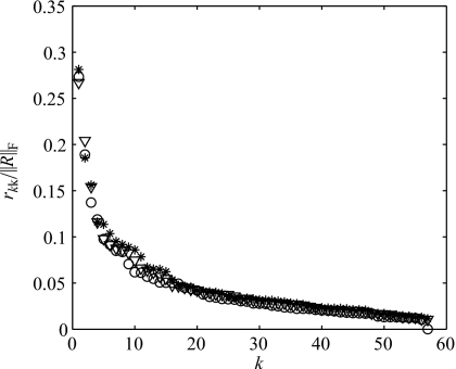
Figure 2 shows the computed R values, normalized to the size of matrix R, for both subjects. In both cases, the values decrease smoothly. In the case of subject S1, there is a sudden drop for the last value, with r_56,56=22.70 mm and r_57,57=0.10 mm. Since the precision of the data is ϵ≈0.5 mm, then for k=56, ‖R₂₂‖₂=∣r_57,57∣⩽ϵ and therefore rank(A)=56. This result indicates that data for one marker are redundant. In fact, it reflects the filling of missing values for the left upper eyelid from the data collected for the right one.

Figure 2.

R values (diagonal elements of matrix R) normalized to the size of R, for subjects S1 (circles), S2a (stars), and S2b (triangles).

In the case of subject S2 (datasets S2a and S2b), there is no gap in the data, and rank(A)=57. Thus, any model built from a subset of less than 56 or 57 markers will necessarily result in a loss of information.

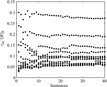
Figure 3 shows the first 12 R values normalized to the size of matrix R, for subject S1, when varying the number of sentences in the dataset. The values stabilize for sets with more than approximately 25 sentences. Any larger data set is therefore reliable enough for building a model. The datasets for subject 2 produce similar results, and are therefore not shown.

Figure 3.

Normalized values of the first 12 R values vs number of sentences in the data set, for subject S1.

Table 1 shows the index of the first 16 columns (or markers) selected by the algorithm, for the various datasets. A set of 30 sentences was used in all analyses.

Table 1.

Selected columns (markers) of data matrix A. For S1, S2a, and S2b, the first 30 sentences of each dataset were used. In case of S2a^* and S2b^*, the last 30 sentences (from a total of 50) of the respective datasets were used.

Order	S1	S2a	S2b	S2a*	S2b*
1	40	40	40	40	40
2	34	34	34	34	34
3	38	13	13	13	11
4	2	38	38	42	38
5	36	47	48	38	56
6	6	42	47	43	42
7	20	6	11	47	6
8	49	56	36	11	47
9	11	11	42	36	13
10	52	36	49	6	36
11	54	48	6	49	12
12	47	39	53	12	48
13	22	52	20	48	39
14	32	20	39	16	16
15	39	49	56	20	53
16	48	14	14	52	20

In all cases, the first selected marker is the 40th, at the center of the lower lip (see Fig. 1), which has therefore the largest displacement (largest 2-norm of the associated column). The second is marker 34, at the lip’s left corner. From the third marker, subject S1 shows a different pattern than subject S2. In the case of subject S1, the next four markers are lip’s right corner (38), right eyebrow (2), upper lip center (36), and left eyebrow (6). Subject S2, on the other hand, besides the lip’ right corner (38), incorporates the eyelids (13 or 11), and markers at the lower-right portion of the face (42, 43, 47, 48, or 56), depending on the dataset. The upper lip marker (6) appears later, in position 8th–10th. The four columns of results for subject S2 show similar markers, although some differences in the selected markers and the order they appear may be noted. For example, looking only at the first seven markers in the perioral region for S2, we note that 6 of them appear in the four data sets: 34, 36, 38, 40, 42, and 47. The remainder marker is 48 (S2b), 56 (S2a and S2b^*), or 43 (S2a^*). Markers 48 and 56 are both at the chin and close together, so they may be considered as belonging to the same facial region. Marker 43, on the other hand, belongs from a different region, close to the right border of the face.

In the case of subject S1, the last selected marker is the 13th (left upper eyelid). Since the algorithm already detected a rank 56 for the data (and therefore a redundant data column), then the data column for that marker is redundant. That result provides a validation of the algorithm, showing its capability to detect artifacts introduced into the data.

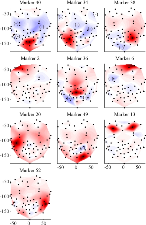
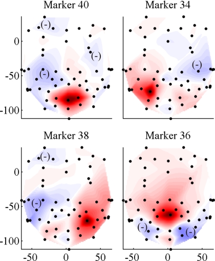
Once the main columns or markers have been selected, a least square fit of the remaining columns may be computed by solving R₁₁X=R₁₂, as explained in the previous section. As a numerical example, a basis of ten independent markers (this number includes up to the lower lip marker in all datasets) was adopted. Figure 4 shows the results of the fit, for subject S1. There the fitting coefficients computed for the secondary markers have been extended to other facial points by cubic interpolation to improve visualization of the results. Note that, in general, the regions associated with each of the markers include both positive and negative subregions, where motion is in the same and opposite direction, respectively, to the marker’s motion. Motion of the each kinematic region is therefore determined by the motion of its associated independent marker, and the total motion of the face is composed by the linear combination of all the kinematic regions. The regions seem to distribute in similar numbers and locations on both sides of the face, although they show a large asymmetry. Regarding the eyelids, although only marker 11 (right eyelid) was identified as an independent marker, marker 13 (left eyelid) has a fit coefficient of 1, which indicates identical motion patterns.

Figure 4.

(Color online) Independent kinematic regions for subject S1, when a basis of ten markers is adopted. The darker the region, the larger the least square fit coefficient of each point relative to the main marker. A minus sign indicates a subregion with negative weight.

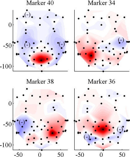
For comparison, regions for subject S2 are shown in Figs. 5 (S2a) and 6 (S2b), which correspond to markers at the center of lower lip, both lip corners, and center of upper lip. Particularly, note that although the upper lip marker appears in different positions in the list of independent markers in Table 1: 8th for S2a and 10th for S2b, the associated regions have similar shapes.

Figure 5.

(Color online) Four independent kinematic regions for subject S2a and for a basis of ten markers. The darker the region, the larger the least square fit coefficient of each point relative to the main marker. A minus sign indicates a subregion with negative weight.

Figure 6.

(Color online) Four independent kinematic regions for subject S2b, and for a basis of ten markers. The darker the region, the larger the least square fit coefficient of each point relative to the main marker. A minus sign indicates a subregion with negative weight.

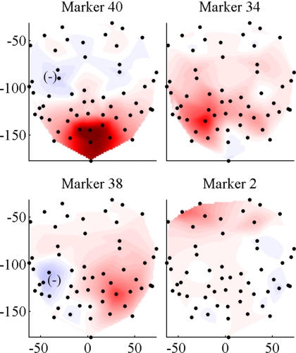
Recall that each marker is selected by the algorithm in a way such that its motion component in a direction orthogonal to the motion of the already selected markers is maximum. The orthogonal directions are represented by the columns of matrix Q, and the components of the markers’s motion in each of the orthogonal directions is given by the rows of matrix R. Figure 7 shows plots of the first four rows of R for subject S1 (related to markers 40, 34, 38, and 2), extended to the whole facial surface by cubic interpolation. The plots therefore represent regions with motion components in the first four orthogonal directions. The first orthogonal direction is given by the jaw-lower lip motion, which has the largest norm, and clearly dominates motion of the lower half of the face. The left lip corner has the largest motion component orthogonal to the lower lip’s motion, and next the right lip corner, with the largest component orthogonal to both the lower lip and the left lip corner. The lip corner regions reflect the mouth widening-narrowing under the combined action of the orbicularis oris, zygomatic major, and other perioral muscles at each side of the face. Naturally, even though motion of both lip corners might be strongly correlated, they are associated with different regions because their motion is controlled by different groups of muscle and happens in opposite directions. This is precisely one of the intended objectives: rather than identifying particular facial gestures such as a mouth widening∕narrowing action, the algorithm identifies spatial regions associated with different muscle groups.

Figure 7.

(Color online) First four orthogonal regions for subject S1. Each plot shows facial points with patterns of motion in the first four orthogonal directions. The darker the region, the larger the motion. A minus sign indicates a subregion with negative weight.

COMPUTER GENERATION OF FACIAL ANIMATIONS

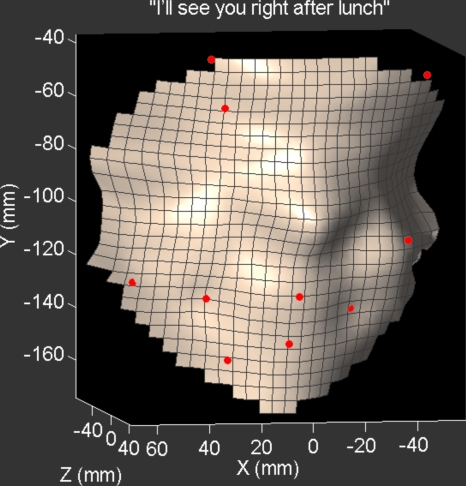
After the main markers and fitting matrix X have been computed, facial animations of arbitrary speech utterances may be produced by driving the selected independent markers with collected signals. Letting P₁∊R^n×k be the displacement matrix of the k main markers (relative to the initial neutral position), then the displacement P₂ of the secondary markers is just P₂=P₁X. The neutral position of all markers is next added back, to obtain their position in head coordinates. Finally, the position of other arbitrary facial points may be generated by using, e.g., cubic interpolation. Using this technique and the results of Table 1, animations were produced for sentences 31–40 for subject S1, and 31–50 for subject S2. A virtual facial surface was generated by cubic interpolation of the recorded markers, built from a grid of 30×30 points. The animations look visually realistic, without any noticeable distortion in the motion pattern. They are available in http:∕∕www.mat.unb.br∕lucero∕facial∕qr2.html in AVI format. Figure 8 shows an example of an animation frame.

Figure 8.

(Color online) Example of a facial animation frame.

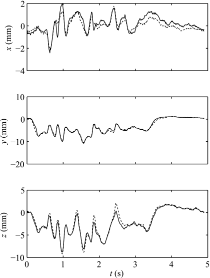
Figure 9 shows the trajectory of marker 56 at the jaw for subject S1 in one sentence (31), when using a basis of ten markers. The plots show that the model recovers the jaw trajectory with good accuracy. The maximum errors are 0.8, 2.0, and 0.9 mm for the x, y, and z directions, respectively.

Figure 9.

Trajectory of marker 56 at the jaw for subject S1 and sentence 31, when using a basis of ten markers. Full line: trajectory computed from the model. Broken line: measured trajectory.

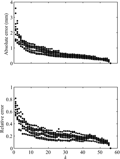
Figure 10 shows the mean error of the computed trajectories when varying the number of independent markers, for both subjects in all the above sentences (the mean error is computed from the secondary markers only). Naturally, the error decreases when the number of markers is increased. The absolute error seems low even with few markers, but at the same time, the relative error seems high. The high relative error is a consequence of the small displacements of most markers.

Figure 10.

Mean error of computed trajectories for subject S1 (sentences 31 to 40) vs number of markers in the selected basis. Top: absolute error. Bottom: relative error.

CONCLUSION

The paper has shown that the QR factorization with column pivoting algorithm provides a convenient technique for facial motion analysis and animation. It identifies a subset of independent facial points (markers), which may be used to build an individualized linear model of facial kinematics. Each of the independent points defines a kinematics region, whose motion is determined by the point’s motion. The total motion of the face is then expressed as the linear combination of the motion of the independent kinematic regions. The regions vary for different subjects, and to some degree, for different data sets. In the studied cases, however, the lower lip and both lip corners tend to be among the first (and therefore most independent) kinematic regions.

Note that the purpose of the technique is not just the reduction of the dimensionality of the data. For that purpose, the singular value decomposition (used in PCA and ICA techniques) is superior, since it permits the computation of the matrix of a given rank k that is closest to the data matrix A. Its disadvantage, for the present modeling objective, is that the computed k-rank matrix is defined in terms of a basis of k eigenvectors (the singular vectors), which do not belong, in general, to the set of column vectors of the original data. The proposed technique, on the other hand, uses a basis formed by column vectors of the data matrix, at the expense of achieving a suboptimal overall dimension reduction. However, as explained in Sec. 1, the PCA and the QR factorization methods are defining DOF differently, and by extension their notion of redundant features of the data are quite different. Thus, the optimality of the dimension reduction needs to be considered in this light. The two analyses are not producing unique decompositions of the data and therefore the residual variances are quite different.

The model has an empirical nature, however, it reflects the underlying biomechanical structure of the face and may be used to infer aspects of that structure. The kinematic regions are the result of the interaction of the muscular driving forces and the the biophysical characteristics of skin tissue. Normally, when building a mathematical model of a given physiological system, one wants to separate out the plant characteristics from the control signals that are instantiated in the muscle activity. The present model, on the other hand, provides a lumped representation of the facial biomechanics.

In biological motion (point light) studies of human gait patterns, the motion is said to contain two sources of information (Troje, 2002): “motion-mediated structural information” and information that is strictly dynamical (e.g., patterns of accelerations and velocities). The human perceptual system is sensitive to both. The point light displays reveal structural information by revealing the rigid body segments and their dimensions as well as showing where the segment joints are. The face is a unique biomechanical system and the analysis of its soft tissue deformations is different from studying articulated motion like locomotion. However, motion patterns of the face can reveal its structural form. In this sense, the proposed technique is carrying out biomechanical analyses of the face. For each individual, it is letting the motions define what regions of the face move as an independent unit, what the boundaries of the surface regions are, and where the spatial peak of motion is located. This can be seen as a lumped representation of the muscular actions and their influence on the facial tissue biophysics.

Many aspects of the technique require further improvement; for example, a criteria to determine the appropriate number of independent markers to be selected is needed. An important issue that must be also considered is that the this modeling approach is dependent on the data captured by the finite set of facial markers. Therefore, building a successful facial model would require researchers to cover a subject’s face densely enough to capture all details of its kinematic behavior, or require researchers to place a smaller number of markers at optimal positions. Those and related issues are currently being considered as next research steps.

References

- Badin, P., Bailly, G., and Revéret, L. (2002). “Three-dimensional linear articulatory modeling of tongue, lips, and face, based on MRI and video images,” J. Phonetics 10.1006/jpho.2002.0166 30, 533–553. [DOI] [Google Scholar]
- Beautemps, D., Badin, P., and Bailly, G. (2001). “Linear degrees of freedom in speech production: Analysis of cineradio- and labio-film data and articulatory-acoustic modeling,” J. Acoust. Soc. Am. 10.1121/1.1361090 109, 2165–2180. [DOI] [PubMed] [Google Scholar]
- Bernstein, N. (1967). The Co-ordination and Regulation of Movements (Pergamon, Oxford: ). [Google Scholar]
- Bischof, C. H., and Quintana-Ort, G. (1998). “Computing rank-revealing QR factorization of dense matrices,” ACM Trans. Math. Softw. 10.1145/290200.287637 24, 226–253. [DOI] [Google Scholar]
- Björck, A. (2004). “The calculation of linear least squares problems,” Acta Numerica 13, 1–53. [Google Scholar]
- Chan, T. F. (1987). “Rank revealing QR factorizations,” Linear Algebr. Appl. 88/89, 67–82. [Google Scholar]
- Chan, T. F., and Hansen, P. C. (1992). “Some applications of the rank revealing QR factorization,” SIAM (Soc. Ind. Appl. Math.) J. Sci. Stat. Comput. 13, 727–741. [Google Scholar]
- Davis, H., and Silverman, S. R., eds. (1970). Hearing and Deafness, 3rd ed. (Holt, Rinehart and Winston, New York: ). [Google Scholar]
- de Hoog, F. R., and Mattheij, R. M. M. (2007). “Subset selection for matrices,” Linear Algebr. Appl. 422, 349–359. [Google Scholar]
- Ekman, P., Friesen, W. V., and Hager, J. C. (2002). The Facial Action Coding System, 2nd ed. (Research Nexus eBook, Salt Lake City: ). [Google Scholar]
- Engwall, O., and Beskow, J. (2003). “Effects of corpus choice on statistical articulatory modeling,” in Proceedings of the 6th International Seminar on Speech Production, edited by Palethorpe S. and Tabain M., pp. 1–6.
- Goldinger, S. D. (1996). “Words and voices: Episodic traces in spoken word identification and recognition memory,” J. Exp. Psychol. Learn. Mem. Cogn. 22, 1166–1183. [DOI] [PubMed] [Google Scholar]
- Golub, G. H., and Loan, C. F. V. (1996). Matrix Computations, 3rd ed. (The Johns Hopkins University Press, Baltimore: ). [Google Scholar]
- Kalra, P., Mangili, A., Thalmann, N. M., and Thalmann, D. (1992). “Simulation of facial muscle actions based on Rational Free Form Deformations,” Comput. Graph. Forum 11, 59–69. [Google Scholar]
- Kanjilal, P., Dey, P. K., and Banerjee, D. N. (1993). “Reduced-size neural networks through singular value decomposition and subset selection,” Electron. Lett. 10.1049/el:19931010 29, 1516–1518. [DOI] [Google Scholar]
- Knappmeyer, B., Thornton, I. M., and Blthoff, H. H. (2003). “The use of facial motion and facial form during the processing of identity,” Vision Res. 43, 1921–1936. [DOI] [PubMed] [Google Scholar]
- Kuratate, T., Munhall, K. G., Rubin, P. E., Vatikiotis-Bateson, E., and Yehia, H. (1999). “Audio-visual synthesis of talking faces from speech production correlates,” in Proceedings of the 6th European Conference on Speech Communication and Technology (EuroSpeech99), Vol. 3, pp. 1279–1282.
- Kuratate, T., Yehia, H., and Vatikiotis-Bateson, E. (1998). “Kinematics-based synthesis of realistic talking faces,” in International Conference on Auditory-Visual Speech Processing (AVSP’98), edited by Burnham D., Robert-Ribes J., and Vatikiotis-Bateson E. (Causal Productions, Terrigal-Sydney, Australia: ), pp. 185–190. [Google Scholar]
- Lawson, C. L., and Hanson, R. J. (1987). Solving Least Squares Problems (SIAM, Philadelphia: ). [Google Scholar]
- Lee, Y., Terzopoulos, D., and Waters, K. (1995). “Realistic modeling for facial animation,” Comput. Graph. 10.1145/204362.204374 29, 55–62. [DOI] [Google Scholar]
- Lorenzelli, F., Hansen, P. C., Chan, T. F., and Yao, K. (1994). “A systolic implementation of the Chan/Foster RRQR algorithm,” IEEE Trans. Signal Process. 42, 2205–2208. [Google Scholar]
- Lucero, J. C., and Munhall, K. G. (1999). “A model of facial biomechanics for speech production,” J. Acoust. Soc. Am. 10.1121/1.428108 106, 2834–2842. [DOI] [PubMed] [Google Scholar]
- Lucero, J. C., Maciel, S. T. R., Johns, D. A., and Munhall, K. G. (2005). “Empirical modeling of human face kinematics during speech using motion clustering,” J. Acoust. Soc. Am. 10.1121/1.1928807 118, 405–409. [DOI] [PubMed] [Google Scholar]
- Migliore, M. D. (2006). “On the role of the number of degrees of freedom of the field in MIMO channels,” IEEE Trans. Antennas Propag. 54, 620–628. [Google Scholar]
- Müller, P., Kalberer, G. A., Proesmans, M., and Van Gool, L. (2005). “Realistic speech animation based on observed 3-D face dynamics,” IEE Proc. Vision Image Signal Process. 10.1049/ip-vis:20045112 152, 491–500. [DOI] [Google Scholar]
- Munhall, K. G., and Vatikiotis-Bateson, E. (1998). “The moving face during speech communication,” in Hearing By Eye, Part 2: The Psychology of Speechreading and Audiovisual Speech, edited by Campbell R., Dodd B., and Burnham D. (Taylor & Francis Psychology, London: ). [Google Scholar]
- Parke, F., and Waters, K. (1996). Computer Facial Animation (AK Peters, Wellesley: ). [Google Scholar]
- Pitermann, M., and Munhall, K. G. (2001). “An inverse dynamics approach to face animation,” J. Acoust. Soc. Am. 10.1121/1.1391240 110, 1570–1580. [DOI] [PubMed] [Google Scholar]
- Prasad, S., and Chandna, B. (1991). “Direction-of-arrival estimation using rank revealing QR factorization,” IEEE Trans. Signal Process. 10.1109/78.80977 39, 1224–1229. [DOI] [Google Scholar]
- Ruckman, C. E., and Fuller, C. R. (1995). “Optimizing actuator locations in active noise control systems using subset selection,” J. Sound Vib. 10.1006/jsvi.1995.0458 186, 395–406. [DOI] [Google Scholar]
- Setnes, M., and Babuska, R. (2001). “Rule base reduction: some comments on the use of orthogonal transforms,” IEEE Trans. Syst. Man Cybern., Part C Appl. Rev. 10.1109/5326.941843 31, 199–206. [DOI] [Google Scholar]
- Terzopoulos, D., and Waters, K. (1990). “Physically-based facial modeling, analysis, and animation,” J. Visual. Comp. Animat. 1, 73–80. [Google Scholar]
- Troje, N. F. (2002). “Decomposing biological motion: A framework for analysis and synthesis of human gait patterns,” J. Vision 2, 371–387. [DOI] [PubMed] [Google Scholar]
- Vatikiotis-Bateson, E., and Yehia, H. (1996). “Physiological modeling of facial motion during speech,” Trans. Tech. Com. Psycho. Physio. Acoust. H-96-65, 1–8. [Google Scholar]