Motion Control of Musculoskeletal Systems with Redundancy

Abstract

Motion control of musculoskeletal systems for functional electrical stimulation (FES) is a challenging problem due to the inherent complexity of the systems. These include being highly nonlinear, strongly coupled, time-varying, time-delayed, and redundant. The redundancy in particular makes it difficult to find an inverse model of the system for control purposes. We have developed a control system for multiple input multiple output (MIMO) redundant musculoskeletal systems with little prior information. The proposed method separates the steady-state properties from the dynamic properties. The dynamic control uses a steady-state inverse model and is implemented with both a PID controller for disturbance rejection and an artificial neural network (ANN) feedforward controller for fast trajectory tracking. A mechanism to control the sum of the muscle excitation levels is also included. To test the performance of the proposed control system, a two degree of freedom ankle-subtalar joint model with eight muscles was used. The simulation results show that separation of steady-state and dynamic control allow small output tracking errors for different reference trajectories such as pseudo-step, sinusoidal and filtered random signals. The proposed control method also demonstrated robustness against system parameter and controller parameter variations. A possible application of this control algorithm is FES control using multiple contact cuff electrodes where mathematical modeling is not feasible and the redundancy makes the control of dynamic movement difficult.

I. Introduction

The loss of volitional motor control of the musculoskeletal system has a variety of causes, including spinal cord injury and neurological diseases. In cases where the peripheral nervous system and musculoskeletal system remain intact, such as in spinal cord injury and stroke, voluntary motion control can be restored by functional electrical stimulation (FES) of the paralyzed muscles or the peripheral nerves innervating the muscles (Peckham and Knutson, 2005). However, developing motion control algorithms for FES is a challenging problem due to the inherent complexities of musculoskeletal systems including highly nonlinear, strongly coupled, time-varying, time-delayed, and redundant properties (Crago et al., 1980). A musculoskeletal system is redundant since the number of muscles acting on a joint is larger than the degrees of freedom of the joint. Although this redundancy enables dexterity in human motor control, it causes difficulty in finding an inverse model of a many-to-one system for control purpose (Jordan and Rumelhart, 1992; Karniel and Inbar, 2000). To resolve the redundancy problem in finding muscle activation levels for FES control, it is typical to use optimization methods with energy consumption as a cost function (Anderson and Pandy, 2001; Pandy, 2001). However, since the optimization process is applied to the computational model not the actual system, modeling error can cause performance degradation of model based approaches.

The non-negligible modeling error of the musculoskeletal systems is due to the complexity of the systems. The most widely used muscle model is the Hill-type muscle model (Zajac, 1989). The Hill-type muscle model has limitations in predicting the muscle behavior during motion because it assumes that muscle activation, length dependent force, and velocity dependent force are independent (Zajac, 1989; Perreault et al., 2003). Although incorporating length-dependent coupling between activation and velocity predicts muscle behavior more accurately over a wide range of motion (Shue and Crago, 1998), its application is limited because there is no noninvasive method to measure individual muscle force directly for the modeling. Due to these limitations in current computational muscle models, black box model based approaches have been often used (Abbas and Triolo, 1997; Chang et al., 1997; Adamczyk and Crago, 2000; Previdi and Carpanzano, 2003; Kurosawa et al., 2005).

In the presence of model uncertainty, feedback control such as PID control can reduce output error. However, the relatively large latency in the musculoskeletal system makes simple feedback control unsuitable for rapid motion control, and so feedforward control is required (Chang et al., 1997; Ferrarin et al., 2001; Kurosawa et al., 2005). A feedforward controller is an inverse model of a system and this inverse model for a redundant system is difficult to obtain using only input-output data. The two most popular methods to resolve redundancy for the training of an inverse model without mathematical modeling are distal teacher method (Jordan and Rumelhart, 1992) and feedback error learning (Kawato et al., 1993). In the distal teacher method, the information of the system output gradient with respect to the system input is stored in the forward model for the training of the inverse model. In feedback error learning, the inverse dynamics is approximated by a feedback controller and the feedback controller output is used to train the inverse model. In both schemes, if the output error surface is complicated, the tracking performance degrades because of inaccurate approximation of the forward dynamics in the distal teacher method and the inverse dynamics in feedback error learning. Therefore, the applications of these approaches using output error for the training of an inverse model have been limited to single joint models with one agonist and one antagonist muscle, where the output gradient with respect to the input is well determined (Riess and Abbas, 2000; Kurosawa et al., 2005).

In order to resolve the redundancy in musculoskeletal systems, Katayama and Kawato suggested that the statics and dynamics should be separated to find the inverse of the system and then placed the inverse static model and inverse dynamic model in series for the control purpose (Katayama and Kawato, 1993; Kawato et al., 1993). However, no practical applications or results have been published.

We have developed a motion control algorithm for redundant multiple input multiple output (MIMO) musculoskeletal systems using only system input-output data. The inverse model is obtained by separating steady-state properties from dynamics properties based on the hypothesis that the steady state inverse model is easier to obtain than the overall inverse model. Since the combination of feedback and feedforward controllers shows better performance than using either a feedback or feedforward controller alone (Chang et al., 1997; Ferrarin et al., 2001; Kurosawa et al., 2005), the proposed control scheme incorporates both artificial neural network (ANN) feedforward controller and PID feedback controller. To test the performance of the proposed control mechanism, we applied the control method to a two degree of freedom ankle-subtalar joint model because of its redundancy and coupling between dorsiflexion/plantar flexion and inversion/eversion.

II. Controller Design

A. Computational model of ankle-subtalar joint

A human computational ankle-subtalar joint model modified from a lower extremity SIMM model was used for the simulation as shown in Fig. 1 (Delp, 1990). The eight Hill-type muscles around ankle-subtalar joints in the model are listed in table 1. Flexor hallucis, flexor digitorum, extensor hallucis, extensor digitorum muscles are not included in this model. The inputs to the model are muscle excitation levels between 0 (no excitation) and 1 (full excitation) and the outputs are angular displacements; dorsiflexion/plantar flexion of the ankle (talocrural) joint and inversion/eversion of the subtalar joint. Dorsiflexion and inversion are defined as the positive direction whereas plantar flexion and eversion are the negative direction. The neutral position is when the foot makes right angle with the shank and there is no inversion or eversion. The ranges of motion determined by passive properties of the joints are roughly from −40° to 30° for the ankle joint and −20° to 20° for the subtalar joint. Due to the effect of gravitational force and limited dorsiflexor muscle force, the range of dorsiflexion is smaller than what is restricted by the passive joint constraint. All the other joints except for the ankle and subtalar joints are fixed. In this model the foot is not supported, and therefore, ground reaction force is not considered. The direction of gravitational force is shown in Fig. 1. For modeling and dynamic simulation of the model, SIMM and SD/FAST were used.

Fig. 1.

Ankle-subtalar joint model with eight muscles and two DOF joint angles. (a) There are eight muscles around ankle-subtalar joints: MG, LG, Sol, TA, TP, PB, PL and PT. The knee joint is fixed and the gravitational direction is parallel to the shank direction. (b) System inputs are muscle excitation levels between 0 and 1. System outputs are angular displacements of ankle joint (dorsiflexion/plantar flexion) and subtalar joint (inversion/eversion).

Table 1.

List of muscles included in the simulation model and their parameters

Muscle name	Maximum muscle force (N)	Optimal fiber length (cm)	Tendon slack length (cm)	Pennation angle (degrees)
Medial gastrocnemius (MG)	1,113	4.5	40.8	17.0
Lateral gastrocnemius (LG)	488	6.4	38.5	8.0
Soleus (Sol)	2,839	3.0	26.8	25.0
Tibialis anterior (TA)	603	9.8	22.3	5.0
Tibialis posterior (TP)	1,270	3.1	31.0	12.0
Peroneus brevis (PB)	348	5.0	16.1	5.0
Peroneus longus (PL)	754	4.9	34.5	10.0
Pernoneus tertius (PT)	90	7.9	10.0	13.0

The ankle-subtalar joint model is highly nonlinear and strongly coupled. A single muscle activation causes both ankle and subtalar joint motion as shown in Fig. 2-(a). Therefore, in many cases, more than one muscle should be activated to generate a desired position. The strong coupling and nonlinearity is also found in the fact that the joint moment depends on the angular displacement of the other joint. For example, the magnitude and the direction of the subtalar joint moment generated by the maximum MG activation strongly depend on the ankle joint angle as shown in Fig. 2-(b). This nonlinearity and coupling makes it difficult for the conventional linear control method to obtain a satisfactory performance.

Fig. 2.

Model analysis. (a) The steady state output joint angles when each of eight muscles is fully activated. (b) An example of strong coupling and nonlinearity properties of the ankle-subtlar joint system. The subtalar joint moments generated by the maximum MG activation with respect to subtalar joint angle variations were calculated for four different ankle joint angles from −30° to 15°. The magnitudes and the direction of the subtalar joint moment depend on the ankle joint angle as well as the subtalar joint angle.

B. Control system structure

The proposed controller is composed of three parts: an inverse steady state controller (ISSC), a feedback controller and a feedforward controller (Fig. 3). ISSC is an inverse model of the system at steady-state and the number of input variables to ISSC is the same as the number of output variables of the system. The information about the inverse dynamics of the system lacking in ISSC is stored in the feedforward controller. The feedforward controller is an ANN trained to be an inverse model of the combination of the system and ISSC. A PID controller is used as the feedback controller and reduces the effects of disturbances and system parameter variation. In this paper we tested two types of control structure: type I and type II controllers. In type I controller (Fig. 3-a), the feedback control is applied to the system through ISSC whereas in type II controller, feedback control is directly applied to the system (Fig. 3-b). Since type II controller uses direct feedback to the system, the number of PID gains to be determined is larger than those of type I controller.

Fig. 3.

Proposed controller structure. The system stands for the ankle-subtalar joint musculoskeletal model. ISSC is the inverse steady state controller. The Feedforward controller is a multilayer perceptron network (MLP) and feedback controller is PID controller. (a) type I controller structure: Both the feedforward and the feedback control are applied through ISSC. (b) type II controller structure: the feedforward control is applied through ISSC and feedback control is applied directly to the system.

C. Inverse steady state controller (ISSC)

A joint angle converges to a certain value when agonist and antagonist muscles around the joint are activated with constant levels (Hogan, 1984). According to the Hill-type muscle model, a muscle is composed of a contractile element in parallel with an elastic viscous element, and a tendon is modeled as an elastic element in series with the muscle (Riener et al., 1996). For isometric contractions, the viscous element does not generate force and the muscle behaves like a nonlinear spring where the spring constant is proportional to muscle activation level. Thus by changing the activation levels of agonist and antagonist muscles, the output joint angle can be controlled (Hogan, 1984). The output joint angles converge for constant muscle excitation levels and the final values do not depend on the initial conditions with some exceptions related to the passive joint property at the boundaries of the range of motion in multi-DOF cases. However, the convergence speed is not uniform and depends on the initial conditions as well as muscle excitation levels. One of the reasons for different convergence speeds is the nonlinear length dependent muscle force property (Zajac, 1989).

The inputs to the ISSC are the desired joint angles and the outputs of ISSC are the muscle excitation levels to make the joint angles converge to the desired steady state values. Although the steady state inverse model is easier to find than the dynamic inverse model, redundancy makes it difficult to obtain an accurate steady state inverse model. Considering the high number of dimensions of the system input space (n=8), it is not plausible to try every possible combination of muscle excitation levels to find the steady state input-output relations. Therefore, it is more reasonable to find the input-output relations from the system output space (joint angle coordinates) whose dimension is much smaller than the input space dimension. To find input-output data sets covering the reachable output angles, linear interpolation of the previously obtained muscle excitation levels with their corresponding output angles are applied to the system repetitively. The linear interpolation method using three points encompassing the desired output in the joint angle coordinate is explained in the appendix A. Because of the nonlinearity of the system, the output joint angles generated by the interpolated muscle excitation level do not coincide exactly with the desired output joint angles. However, the repetitive trials can generate input-output data covering the reachable output coordinate space. One benefit of using linear interpolation is that the sum of each muscle excitation level remains unchanged after interpolation as long as the muscle excitation levels used for the interpolation have the same sum. The sum of the muscle excitation levels is defined as the total activation level.

In order to obtain the steady state input-output relations, it is not practical to wait indefinitely until the output joint angles converge for constant muscle excitation. Therefore, we define quasi-steady state output as the output angles 3 seconds after constant muscle excitation. The initial conditions are zero muscle excitation and its corresponding output joint angles, which are −22.5° for the ankle joint and −1.7° for the subtalar joint. The muscle excitation level varies between 0 and 1 with a resolution of 0.01 and the output angle resolution for feedback is set to 1/4°.

The ISSC is composed of a table with 11 levels for dorsiflexion/plantar flexion from −40° to 10°, and 9 levels for inversion/eversion from −20° to 20° making the total number of entry points 11×9 = 99. The muscle excitation levels of each entry in the table are obtained by interpolating the input-output data enclosing the entry point in the joint angle coordinate. If there is no input-output data enclosing the entry point, the muscle excitation levels with higher total activation level are selected. During the control stage, the output of ISSC is the muscle excitation levels using bilinear interpolation of the four nearest entries to the desired output joint angles.

D. Feedforward controller

The role of the feedforward controller is to reshape the input to the ISSC in order to compensate for dynamics information lacking in the ISSC. The feedforward controller was implemented as a feedforward multilayer perceptron (MLP) network with one hidden layer consisting of 30 nodes. Hyperbolic tangent sigmoid functions and linear functions were used for the hidden layer and output layer transfer functions respectively. The input to the feedforward controller at time t was the time series of the future desired output trajectory as follows:

$$[y_d(t+T),y_d(t+2T),y_d(t+3T),y_d(t+4T),y_d(t+5T)],$$

where the sampling period T is set to 20ms.

The feedforward controller was trained with a direct inverse training method, where the system output became the ANN input, and the system input became the ANN output. Pseudo-random signals and pseudo step signals with a 3 minute window were used for the training of the ANN and another 1 minute window was used for validation. Pseudo-random signals were generated by filtering random signals with fourth order Butterworth low-pass filter with cut-off frequency 1Hz. Pseudo-step signals were step signals with smooth transitions between constant values. As a training method of the ANN, Levenberg-Marquardt algorithm was used as ‘trainlm’ in MATLAB.

E. Feedback controller

For the feedback controller, a discrete time PID controller described by the following equations was used:

$$\begin{array}{l}e(t)=y^d(t)-y(t)\\ u_p(t)=K_{p}e(t)\\ u_i(t)=u_i(t-1)+K_{i}e(t)\\ u_d(t)=0.5u_d(t-1)+0.5K_d(e(t)-e(t-1))\\ u_{fb}(t)=u_p(t)+u_i(t)+u_d(t),\end{array}$$ (1)

where u _fb (t) is feedback controller output at time t, y^d is the desired output, y is the system output, and the sampling period is 20ms. u_p, u_i and u_d are proportional, integral and derivative control outputs, and K_p, K_i and K_d are the proportional, integral and derivative gain respectively. A first order filter was used to reduce the noise effect of the derivative control. To prevent the integral control from increasing too much and causing saturation, the integral control output was bounded as described in the following equation.

$$u_i(t)=\{\begin{array}{cc}\hfill -10\hfill & \hfill u_i(t)<-10\hfill \\ \hfill 10\hfill & \hfill u_i(t)>10\hfill \end{array}$$ (2)

The feedback gains of the type I controller were set based on trial and error as follows.

$$K_p=\left[\begin{array}{ll}2\hfill & 0\hfill \\ 0\hfill & 2\hfill \end{array}\right]K_i=\left[\begin{array}{cc}0.1& 0\\ 0& 0.1\end{array}\right]K_d=\left[\begin{array}{ll}2\hfill & 0\hfill \\ 0\hfill & 2\hfill \end{array}\right]$$ (3)

The feedback gains of type II controller were also set based on trial and error as follows.

$$\begin{array}{l}{K}_p={\left[\begin{array}{cccccccc}\hfill -0.01\hfill & \hfill -0.01\hfill & \hfill -0.01\hfill & \hfill 0.02\hfill & \hfill -0.01\hfill & \hfill 0\hfill & \hfill 0\hfill & \hfill 0\hfill \\ \hfill 0\hfill & \hfill 0\hfill & \hfill 0\hfill & \hfill 0.01\hfill & \hfill 0.01\hfill & \hfill -0.01\hfill & \hfill -0.01\hfill & \hfill -0.01\hfill \end{array}\right]}^T\\ K_i=0.01K_p\\ K_d=K_p\end{array}$$ (4)

F. The control of the sum of muscle excitation levels

By combining ISSCs with different total activation levels, it is possible to control the total activation level dynamically during the movement (Fig. 4). An ISSC with a low total activation level can reduce metabolic energy expenditure, while an ISSC with a higher level can increase stiffness and reduce the effect of external disturbances. The level controller interpolates linearly the outputs of these ISSCs as described in the following equations.

Fig. 4.

Control structure with desired coactivation level input. ISSC_n is n-th inverse steady state controller. Each ISSC is built with different coactivation level. FF_n is feedforward controller for ISSC_n. The coactivation controller interpolates the output of ISSCs based on the desired coactivation reference trajectory. (a) type I controller. The sum of feedback controller output and FF_n output is the input to ISSC_n. (b) type II controller. Only feedforward controller output is fed through ISSC and feedback control is directly applied to the system.

$$a(t)=\{\begin{array}{ll}{a}_1(t)\hfill & (c<c_1)\hfill \\ \frac{c_{k+1}-c}{c_{k+1}-c_k}{a}_k(t)+\frac{c-c_k}{c_{k+1}-c_k}{a}_{k+1}(t)\hfill & (c_k\le c<c_{k+1})\hfill \\ a_n(t)\hfill & (c\ge c_n)\hfill \end{array}$$ (5)

Here, a(t) is the output of the level controller, a_k (t) is the output of ISSC_k, a_{k + 1}(t) is the output of ISSC_k+1, c_k is the total activation level of ISSC_k, c_{k +1} is the level of ISSC_k+1, and c is the desired total activation level.

The system output error using the type I or type II controllers in Fig. 4 can be kept small if the output error using each of ISSC_k and ISSC_k+1 is small and the linear approximation error of the system is small in the region. The proof is shown in appendix B.

III. Simulation Results

A. Controller performance

The performance of ISSCs was measured for 100 randomly selected desired positions with 10 random initial positions for each desired position. The standard deviation of the outputs at each desired position with different initial positions decreased rapidly over time indicating the convergence of the system output regardless of the initial positions. Although ISSC with a higher total activation level showed faster convergence rate, more than 85% of the standard deviation of the output errors became less 1° within 3 seconds in all of the ISSCs with four different total activation levels (0.25, 0.50, 0.75, 1.00). The average steady state output errors were less than 2° for both the ankle and subtalar joints.

In order to determine the effect of each component of the controller on the overall performance, the four different control structures were compared using sinusoidal signals: ISSC alone (Fig. 5-a), ISSC with feedforward controller (Fig. 5-b), ISSC with feedback controller (Fig. 5-c), and feedback controller only for the type II controller (Fig. 5-d). The ankle and subtalar joint root mean square (RMS) tracking errors were 15.1° (30.2%) and 9.2° (23.0%) for ISSC alone, 7.0° (14.0%), and 4.7° (11.8%) for feedback control with ISSC, 3.7° (7.4%) and 4.4° (11.0%) for direct feedback control, and 3.0° (6.0%) and 2.4° (6.0%) for feedforward control with ISSC. The tracking errors using ISSC alone were large because ISSC contains information only about steady states. The addition of the feedback controller with ISSC reduced the tracking errors. Direct feedback control performed better than feedback through ISSC. However, the performance of a linear PID controller changed over the desired output range. The feedforward controller improved tracking performance using time series of the future reference trajectories. By incorporating feedback and feedforward controllers together with ISSC, the output error became the smallest. The RMS errors of type I control were 2.0° (4.0 %) for dorsiflexion/plantar flexion and 1.2° (3.0%) for inversion/eversion. The RMS errors of type II control were 1.9° (3.8% error) for dorsiflexion/plantar flexion and 1.1° (2.8% error) for inversion/eversion.

Fig. 5.

System output for the sinusoidal reference trajectories with coactivation level 0.25. (a) ISSC only (b) feedback + ISSC (type I feedback) (c) direct feedback (type II feedback) (d) feedforward + ISSC (e) type I control (f) type II control. The incorporation of feedback and feedforward control with ISSC in type I and type II control performs better than feedback and feedforward control is used separately.

In addition to sinusoidal signals, pseudo-random signals and pseudo-step signals were used to compare the performance of type I and type II controller. Pseudo-random signals are low pass filtered random signals and pseudo-step signals are a series of step signals with smooth transition. The results in Fig. 6 show that both Type I and type II control system can track the reference trajectories within 3% RMS errors for both dorsiflexion/plantar flexion and inversion/eversion.

Fig. 6.

Results of type I and type II control with the total activation level 0.25 for (a) pseudo-step reference trajectories and (b) pseudo-random trajectories. E1 and E2 stand for ankle and subtalar joint RMS errors in degrees respectively. (a) Type I E1: 0.7°(1.4%) E2: 0.6° (1.5%), type II E1: 0.4° (0.8%) E2: 0.6° (1.5%) (b) type I E1: 1.2° (2.4%) E2: 0.8° (2.0%), type II E1: 0.8° (1.6%) E2: 0.6° (1.5%).

B. The frequency response of the proposed control mechanism

In order to test the tracking performance of the proposed controllers depending on the frequency components of the reference trajectories, sinusoidal signals with 3 different frequencies (0.5Hz, 1.0Hz, and 1.5Hz) were selected as desired output trajectories. Although the output errors at low frequencies were small, the performance of both type I and type II degraded for high frequency (1.5Hz) reference trajectories as shown in Fig. 7 because the feedforward controller was not trained for that range of fast movement and the response of feedback control is slow. Fig. 7-(b) shows the corresponding muscle excitation levels generated by the type I controller for the given reference trajectory. When the input to the ISSC is beyond the reachable range of the ISSC with a given total activation level, ISSC with higher level is adopted. For this reason, the muscle excitation levels for fast movement are higher than those for slow movement in Fig. 7-(b).

Fig. 7.

Results of type I and type II control with for in-phase sinusoidal reference trajectories with the total activation level 0.25. (a) The output angles and errors of each joint. E1 and E2 stand for ankle and subtalar joint RMS errors in degrees respectively. Type I control E1: 1.4° (2.8%) for 0.5Hz, 3.0° (4.5%) for 1.0Hz, 8.3° (16.6%) for 1.5Hz, E2: 0.8° (2.0%) for 0.5Hz, 1.6° (4.0%) for 1.0Hz, 3.8° (9.5%) for 1.5Hz, Type II control E1: 1.0° (2.0%) for 0.5Hz, 1.9° (3.8%) for 1.0Hz, 5.0° (10.0%) for 1.5Hz, E2: 1.0° (2.5%) for 0.5Hz, 1.8° (4.5%) for 1.0Hz, 3.5° (8.8%) for 1.5Hz. As the frequency increases, the error increases as well. (b) The corresponding muscle excitation levels generated by type I controller. Muscle excitation levels increase for fast movement

The results for four different levels (0.25, 0.50, 0.75, 1.00) are summarized in table 2 where the sinusoidal reference trajectories with the same magnitude as in Fig. 7 and four different phase difference between the ankle and subtalar joint angles: 0°, 90°, 180° and 270°. The results indicate that the output error increases as the desired motion becomes faster for all levels.

Table 2.

The average and standard deviation of RMS errors for the sinusoidal reference trajectories with four different phase difference between ankle and subtalar joint reference trajectories: 0°, 90°, 180° and 270°. The magnitude of the reference trajectory is the same as the one in Fig. 7. As the frequency component of the reference trajectory increases, the output tracking error increases too

Frequency (Hz)	Total activation level
	0.25	0.50	0.75	1.00
Ankle joint with type I control
0.5	1.5 ± 0.5 (3.0%)	1.5 ± 0.3 (3.0%)	0.9 ± 0.2 (1.8%)	0.8 ± 0.2 (1.6%)
1.0	3.8 ± 1.2 (7.6%)	3.6 ± 1.4 (7.2%)	3.2 ± 0.9 (6.4%)	3.0 ± 0.3 (6.0%)
1.5	8.2 ± 1.5 (16.4%)	7.4 ± 3.0 (14.8%)	6.0 ± 1.2 (12.0%)	6.1 ± 1.4 (12.2%)
Subtalar joint with type I control
0.5	1.2 ± 0.4 (3.0%)	0.7 ± 0.1 (1.8%)	0.8 ± 0.4 (2.0%)	0.7 ± 0.3 (1.8%)
1.0	2.2 ± 0.6 (5.5%)	1.4 ± 0.1 (3.5%)	2.1 ± 0.9 (5.3%)	1.9 ± 0.5 (4.8%)
1.5	4.1 ± 0.8 (10.3%)	2.9 ± 0.9 (7.3%)	3.6 ± 1.3 (9.0%)	3.2 ± 1.2 (8.0%)
Ankle joint with type II control
0.5	1.0 ± 0.1 (2.0%)	1.2 ± 0.3 (2.4%)	0.8 ± 0.1 (1.6%)	0.8 ± 0.1 (1.6%)
1.0	2.0 ± 0.3 (4.0%)	2.6 ± 0.5 (5.2%)	2.2 ± 0.5 (4.4%)	2.5 ± 0.3 (5.0%)
1.5	5.8 ± 0.5 (11.6%)	5.4 ± 1.1 (10.8%)	5.3 ± 0.3 (10.6%)	5.2 ± 0.3 (10.4%)
Subtalar joint with type II control
0.5	1.0 ± 0.2 (2.5%)	0.8 ± 0.1 (2.0%)	0.7 ± 0.2 (1.8%)	0.6 ±0.1 (1.5%)
1.0	2.0 ± 0.3 (5.0%)	1.7 ± 0.3 (4.3%)	1.6 ± 0.2 (4.0%)	1.5 ± 0.5 (3.8%)
1.5	4.1 ± 0.5 (10.3%)	3.8 ± 0.8 (9.5%)	3.4 ± 0.6 (8.5%)	3.3 ± 0.9 (8.3%)

C. Control parameter sensitivity analysis

In order to test the efficacy of building ISSCs using interpolation, we compared the proposed algorithm to an optimization method. For the optimization method, sequential quadratic programming was chosen to find the muscle excitation levels at 99 entry positions of ISSCs. The cost function was the output error from 2 seconds to 10 seconds after the initiation of the stimulation and the sum of the muscle excitation levels were kept constant. The quasi-steady state output errors at 3 seconds after muscle activation with zero initial conditions were obtained for 357 uniformly distributed positions. The average ankle and subtalar joint errors were 0.6° and 0.5° compared to 1.3° and 1.1° of ISSC obtained by the interpolation method. However, the optimization method requires a large number of iterations and therefore is not practical for applications with unknown system dynamics.

To estimate the robustness of the controller performance with the variations of the ANN parameters, different ANN input patterns [y_d (t + T),···, y_d (t +nT)] were tested, where the sampling period T varies from 20ms to 60ms and the number of time delay terms (n) varied from 2 to 5. ISSC with the total activation level 1.0 in the previous section was used and the training signal and method were the same for all the ANNs. A filtered random signal with 3 minute duration was used to test their performance, and the performance variation due to ANN input parameter variation within the tested range was less than a degree indicating the robustness of the proposed controller against the ANN input parameter variations. The performance variation with respect to the number of nodes or layers was not tested here, and the performance could be improved by changing the structure and training method of the ANN controller.

D. Effects of the system parameter variations on the controller performance

Since the maximum muscle strength changes over time due to fatigue, the robustness of the control mechanism for variations of the maximum muscle strength was also tested. The maximum muscle strength of each muscle was decreased by 25% ~ 75% from its original value and 50 different random trials were tested with same pseudo-random reference trajectory in Fig. 6-(b) for each level. The mean and the standard deviation of the tracking error are listed in table 3. The average RMS output errors are less than 4% for both type I and type II controllers for all levels. The performance of the proposed controller did not degrade much with significant change in the muscle parameters because feedback control compensated for the system parameter variation. These results indicate that the proposed controllers are robust against maximum muscle strength change.

Table 3.

The average and standard deviation of RMS errors for the system with maximum muscle strength variations in degrees and percentile error. Each muscle maximum strength decreases randomly with uniform distribution between 25% and 75% and a total of 50 random trials were tested for each of four different total activation level in (a) type I control and (b) type n control. The reference trajectories are pseudo-random signals in Fig. 6-(b). The results show that the effect of the maximum muscle strength change on the output tracking error is not significant indicating the robustness of the proposed control

Angles	Total activation level
	0.25	0.50	0.75	1.00
Type I control
Ankle joint (before change)	1.2 (2.4%)	0.9 (1.8%)	0.7 (1.4%)	0.5 (1.4%)
Ankle joint (after change)	1.6 ± 0.3 (3.2%)	1.4 ± 0.2 (2.8%)	1.1 ± 0.2 (2.2%)	0.9 ± 0.3 (1.8%)
Subtalar joint (before change)	0.8 (2.0%)	0.7 (1.8%)	0.7 (1.8%)	0.6 (1.5%)
Subtalar joint (after change)	1.1 ± 0.3 (2.8%)	1.0 ± 0.2 (2.8%)	1.0 ± 0.2 (2.5%)	1.0 ± 0.2 (2.5%)
Type II control
Ankle joint (before change)	0.8 (1.6%)	0.7 (1.4%)	0.6 (1.2%)	0.5 (1.0%)
Ankle joint (after change)	1.1 ± 0.1 (2.2%)	1.0 ± 0.1 (2.0%)	0.9 ± 0.1 (1.8%)	0.8 ± 0.1 (1.6%)
Subtalar joint (before change)	0.6 (1.5%)	0.5 (1.3%)	0.5 (1.3%)	0.5 (0.5%)
Subtalar joint (after change)	0.9 ± 0.2 (2.3%)	0.8 ± 0.1 (2.0%)	0.8 ± 0.2 (2.0%)	0.9 ± 0.2 (2.3%)

E. Dynamic total activation level change

The tracking performance of the type I and type II controllers has been tested for random reference trajectories and random desired total activation level and is shown in Fig. 8. The results show that the system outputs follow the desired trajectories while maintaining the desired total activation level in both the type I and type II controller. The linear interpolation between ISSCs with different levels did not increase output errors compared to a fixed level. The level control can be used to reduce the effect of external disturbance on the output error which will be shown in the next section.

Fig. 8.

Tracking performance of (a) type I and (b) type II controller while maintaining the desired total activation level. The RMS output errors of type I control are 0.8° (1.6%)and 0.8° (2.0%) for ankle and subtalar joint respectively, and the RMS output errors of type II control are 0.6° (1.2%) and 0.5° (1.3%) for ankle and subtalar joint respectively.

F. Effect of external disturbances

To test the effect of external disturbance on the performance of the type I controller, a 50N external force in the dorsiflexion direction was applied at the point 20 cm from the subtalar joint along the foot as shown in Fig. 1. This external force is equivalent to a 10Nm torque in the dorsiflexion direction and the magnitude is considerable compared to the maximum dorsiflexor torque, which is from 30 to 55Nm in the experiment (Weiss et al., 1986). The disturbance was applied between 5 seconds and 15 seconds and the results are shown in Fig. 9. There were significant output errors due to the strong external disturbance for a low total activation level. High total activation level increases joint stiffness and thus reduces the effects of the external disturbance on the output error. Since the feedback control in the type II controller is not confined to the muscle activation levels determined by ISSCs, the effect of external disturbance in type II control is reduced compared to type I control as shown in Fig. 9-(b) at the expense of diverging from the desired total activation level. Therefore, type II controller is generally more robust against external disturbances than type I controller.

Fig. 9.

Tracking performance of (a) type I and (b) type II controller in the presence of external disturbance. The external disturbance with the magnitude of 50N is applied at a point 20 cm from the subtalar joint along the foot as shown in Fig. 1 between 5 seconds and 15 seconds. As the total activation level increases from low level (0.25) to high level (1.00), the effect of external disturbance on the output error is reduced. Type II controller is more robust against external disturbance because the output of feedback is not restricted to the subspace of ISSCs.

Discussion

The proposed control separating statics from dynamics to find an inverse model of a redundant musculoskeletal system shows satisfactory reference trajectory tracking performance. Compared with the model based approaches (Anderson and Pandy, 2001; Pandy, 2001), our design does not require the time consuming subject dependent modeling procedure, and thus the performance does not depend on the modeling error. Since finding an inverse dynamics model of a redundant nonlinear MIMO musculoskeletal system without using a mathematical description of the model is very difficult, a method to find an inverse model for steady states was employed using only empirical input-output data. The steady state inverse model reduces the dimensionality and makes it feasible to find a dynamic inverse model using ANNs. ISSC stores steady state inverse relations in a table, and the feedforward controller stores dynamic information in an ANN. The combination of the feedforward controller and the ISSC makes a dynamic inverse model. In this way, black box model based control such as using an ANN (Chang et al., 1997) can be easily extended to redundant MIMO musculoskeletal systems.

The proposed algorithm interpolates pre-existing input-output data iteratively to find ISSC. The principal function of ISSC is to make the number of input variables to ISSC be the same as the number of system output variables, and thus reduce the redundancy. Since ISSCs are an approximation of the inverse steady state model, the errors do not converge to zero for several reasons. First, muscle excitation levels are linearly interpolated for a nonlinear function. Second, the output angles at 3 seconds after constant excitation are selected as quasi-steady state outputs instead of waiting until the output angles converge when input-output data are collected to build ISSCs. Third, there are quantization errors in the muscle excitation levels. In sensitive regions where a small change in muscle excitation level can generate large changes in the output angles, the errors due to quantization are not negligible.

For the control of dynamic movement, both feedback and feedforward control are used. The feedforward controller is used for fast trajectory tracking and feedback controller reduces the error even in the presence of internal and external disturbances. For the training of the feedforward ANN controller, the direct inverse training method was adopted for simplicity and convergence despite its limitations compared to the indirect inverse training method (Jordan and Rumelhart, 1992; Karniel et al, 2001).

We compared two types of controllers: type I and type II. In the type I controller, feedback control is applied to the system indirectly through ISSC, while in the type II controller feedback control is fed directly to the system.

The validity of the proposed control system was tested on a human ankle-subtalar joint model with 8 muscles and 2 DOF output angles. The model is redundant with strong coupling between dorsiflexion/plantar flexion and inversion/eversion. The ISSC alone or feedback controller with ISSC in type I control showed relatively large output error and phase lag. The feedback controller alone showed better tracking performance but the performance of linear controller was not uniform for the different joint angles. The feedforward control reduces the output error by compensating for the slow dynamics of ISSCs using time series of the future desired trajectory. The proposed control system combining feedback and feedforward controller could accurately track various reference trajectories including sinusoidal, pseudo-step and pseudo-random signals. Due to feedback control, the proposed controller showed robustness against maximum muscle strength changes due to muscle fatigue.

Although the joint stiffness is not linearly proportional to the total muscle activation level, the joint stiffness is roughly controlled by the muscle co-contraction level by means of the total activation level. Maintaining the same position with a higher total activation level indicates higher activation of the muscles increasing co-contraction. By using multiple ISSCs with different levels and their corresponding feedforward controllers, the total activation level could be controlled dynamically. The effect of the external disturbance was drastically reduced by using high total activation level. In type II control, the effect of an external disturbance on the output error is smaller than in type I control especially at a low total activation level at the expense of deviation from the desired level since the feedback control is not restricted to the subspace generated by ISSC. However, the feedback gains of type II control is more difficult to find than those of type I control because of larger size of the gain matrices.

Since the proposed control algorithm requires only input-output data, it can be applied to functional electrical stimulation where the modeling is difficult or the modeling error is large. For instance, in the case of peripheral nerve stimulation to restore motion with multi-contact nerve cuff electrodes using multi-contact nerve cuff electrodes with fascicular selectivity (Qi et al., 1999), the information about fascicular distribution inside a nerve trunk is required to build a model from the stimulation input to the joint angular displacement output. Since a non-invasive method to determine the fascicular distribution inside a nerve trunk is not available at this moment, the proposed control algorithm can be applicable since it does not require a known model of the plant.

In conclusion, the proposed algorithm provides a robust method to control systems that have significant redundancy and where an accurate model of the system cannot be obtained. In particular, this controller will be applied to the control of musculoskeletal systems with multiple contact nerve cuff electrodes.

Abbreviations

FES

functional electrical stimulation

MIMO

multiple input multiple output

ANN

artificial neural network

MLP

multi-layer perceptron

Appendix A. Finding excitation levels using linear interpolation of three points

Since a triangle is a convex polygon, the nearest three points encompassing a desired point are adopted for linear interpolation. Suppose there are three points p₁, p₂ and p₃ obtained in the previous trials with their corresponding excitation levels a₁, a₂ and a₃ as shown in Fig. 10, where

Fig. 10.

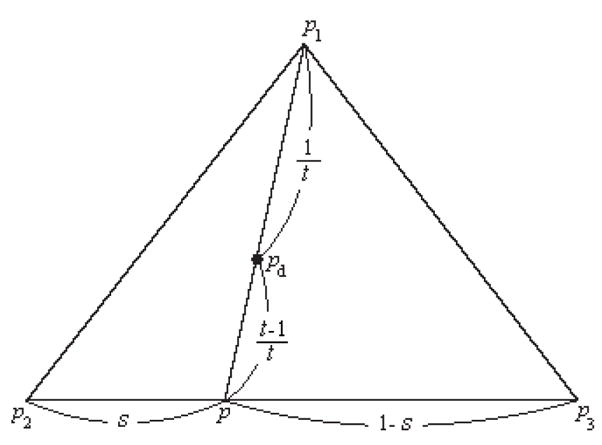
Illustration of the method for finding muscle excitation levels at the desired point p_d using linear interpolation of p₁, p₂ and p₃.

$$p_1=(x_1,y_1),p_2=(x_2,y_2),p_3=(x_3,y_3),p_d=(x_d,y_d).$$

Then the excitation level a_d at the desired point p_d can be obtained using linear interpolation of the excitation levels of the three points as described in the following equation.

$$a_d=a_1+\frac{1}{t}[a_2-a_1+s(a_3-a_2)]$$ (A.1)

$$\begin{array}{l}s=\frac{(x_2-x_1)(y_d-y_1)-(x_d-x_1)(y_2-y_1)}{(x_2-x_3)(y_d-y_1)-(x_d-x_1)(y_2-y_3)}\\ t=\frac{(x_2-x_3)(y_2-y_1)-(x_2-x_1)(y_2-y_3)}{(x_2-x_3)(y_d-y_1)-(x_d-x_1)(y_2-y_3)}\end{array}$$ (A.2)

Proof

The equation of a line connecting p₁ and p_d is

$$p=p_1+t(p_d-p_1),$$ (A.3)

where t is a scalar.

The equation of a line connecting p₂ and p₃ is

$$p=p_2+s(p_3-p_2),$$ (A.4)

where s is a scalar.

These two lines, (A.3) and (A.4), intersect at point p.

$$p=p_1+t(p_d-p_1)=p_2+s(p_3-p_2)$$ (A.5)

From equation (A.5), p_d can be expressed as a function of p₁, p₂ and p₃.

$$p_d=p_1+\frac{1}{t}[p_2-p_1+s(p_3-p_2)]$$ (A.6)

Therefore, the excitation levels at the desired point can be obtained from the excitation levels of the three points in the following equation.

$$a_d=a_1+\frac{1}{t}[a_2-a_1+s(a_3-a_2)]$$ (A.7)

Scalar values s and t are found by solving equation (A.5) or the rephrased following equation.

$$\begin{array}{l}s(x_2-x_3)+t(x_d-x_1)=x_2-x_1\\ s(y_2-y_3)+t(y_d-y_1)=y_2-y_1\end{array}$$ (A.8)

The solution of equation (A.8) is

$$\begin{array}{l}s=\frac{(x_2-x_1)(y_d-y_1)-(x_d-x_1)(y_2-y_1)}{(x_2-x_3)(y_d-y_1)-(x_d-x_1)(y_2-y_3)}\\ t=\frac{(x_2-x_3)(y_2-y_1)-(x_2-x_1)(y_2-y_3)}{(x_2-x_3)(y_d-y_1)-(x_d-x_1)(y_2-y_3)}\end{array}$$ (A.9)

Appendix B. Convergence of type I control

In type I control with the level controller in Fig. 4, let a_k (t) and a_{k +1}(t) be the outputs of ISSC_k and ISSC_k+1 respectively and y(t) be the system output for the current state x(t) and the input a(t) as described in the following equation.

$$y(t)=f(x(t),a(t))$$ (B.1)

If the output errors for the inputs a_k (t) and a_{k +1}(t) are less than ε₁ and ε₂ respectively, then the output error for the input a(t), which is the linear interpolation of a_k (t) and a_{k +1}(t), can be made smaller than ε = max(ε₁, ε ₂ ) + δ. δ is the affine linear approximation error of f (x(t), a(t)) using f (x(t), a_k(t)) and f (x(t), a_k+1 (t)).

Proof

Let the desired total activation level be c (c_k ≤c ≤c_k+1), then the output of the level controller is

$$a(t)=w{a}_k(t)+(1-w)a_{k+1}(t),$$ (B.2)

where $0\le w=\frac{c_{k+1}-c}{c_{k+1}-c_k}\le 1$.

Let y_k (t) and y_{k +1}(t) be the system outputs for the inputs a_k (t) and a_{k +1}(t) respectively, and assume the output errors for these inputs are less than ε₁ and ε₂ with the desired output y^d (t).

$$\begin{array}{l}\parallel y^d(t)-y_k(t)\parallel =\parallel y^d(t)-f(x(t),a_k(t))\parallel <{\epsilon }_1\\ \parallel y^d(t)-y_{k+1}(t)\parallel =\parallel y^d(t)-f(x(t),a_{k+1}(t))\parallel <{\epsilon }_2\end{array}$$ (B.3)

Let the affine linear approximation error for the input a(t) in (B.2) using a_k (t) and a_{k +1}(t) be less than δ as follows.

$$\begin{array}{l}\parallel y(t)-w{y}_k(t)-(1-w)y_{k+1}(t)\parallel \\ =\parallel f(x(t),a(t))-wf(x(t),a_k(t))-(1-w)f(x(t),a_{k+1}(t))\parallel \le \delta \end{array}$$ (B.4)

Then the output error for the interpolated input a(t) is less than ε = max(ε₁, ε₂) + δ from the following equation.

$$\begin{array}{l}\parallel y^d(t)-y(t)\parallel =\parallel y^d(t)-w{y}_k(t)-(1-w)y_{k+1}(t)+w{y}_k(t)+(1-w)y_{k+1}(t)-y(t)\parallel \\ \le \parallel y^d(t)-w{y}_k(t)-(1-w)y_{k+1}(t)\parallel +\parallel y(t)-w{y}_k(t)-(1-w)y_{k+1}(t)\parallel \\ \le \parallel y^d(t)-w{y}_k(t)-(1-w)y_{k+1}(t)\parallel +\delta \\ =\parallel (w+1-w)y^d(t)-w{y}_k(t)-(1-w)y_{k+1}(t)\parallel +\delta \\ =\parallel w\left(y^d(t)-y_k(t)\right)-(1-w)\left(y^d(t)-y_{k+1}(t)\right)\parallel +\delta \\ \le w\parallel y^d(t)-y_k(t)\parallel +(1-w)\parallel y^d(t)-y_{k+1}(t)\parallel +\delta \\ <w{\epsilon }_1+(1-w){\epsilon }_2+\delta \\ \le wmax({\epsilon }_1,{\epsilon }_2)+(1-w)max({\epsilon }_1,{\epsilon }_2)+\delta \\ =max({\epsilon }_1,{\epsilon }_2)+\delta \le \epsilon \end{array}$$ (B.5)

In a similar way, it can be proved that type II control with level control makes the output error small if each ISSC controller can make the output error small.

References

- Abbas JJ, Triolo RJ. Experimental evaluation of an adaptive feedforward controller for use in functional neuromuscular stimulation systems. IEEE Transactions on Rehabilitation Engineering. 1997;5:12–22. doi: 10.1109/86.559345. [DOI] [PubMed] [Google Scholar]
- Adamczyk MM, Crago PE. Simulated feedforward neural network coordiantion of hand grasp and wrist angle in a neuroprosthesis. IEEE Transactions on Rehabilitation Engineering. 2000;8:297–304. doi: 10.1109/86.867871. [DOI] [PubMed] [Google Scholar]
- Anderson FC, Pandy MG. Static and dynamic optimization solutions for gait are practically equivalent. Journal of Biomechanics. 2001;34:153–161. doi: 10.1016/s0021-9290(00)00155-x. [DOI] [PubMed] [Google Scholar]
- Chang G-C, Lub J-J, Liao G-D, Lai J-S, Cheng C-K, Kuo B-L, Kuo T-S. A neuro-control system for the knee joint position control with quadriceps stimulation. Rehabilitation Engineering, IEEE Transactions on. 1997;5:2–11. [PubMed] [Google Scholar]
- Crago PE, Peckham PH, Thrope GB. Modulation of muscle force by recruitment during intramuscular stimulation. Ieee Transactions on Biomedical Engineering. 1980;27:679–684. doi: 10.1109/TBME.1980.326592. [DOI] [PubMed] [Google Scholar]
- Delp SL. Surgical simulation : A computer graphics system to analyze and design musculoskeletal reconstructions of the lower limb. PhD Dissertation, Stanford 1990 [Google Scholar]
- Ferrarin M, Palazzo F, Riener R, Quintern J. Model-based control of fes-induced single joint movements. Neural Systems and Rehabilitation Engineering. IEEE Transactions on [see also IEEE Trans on Rehabilitation Engineering] 2001;9:245–257. doi: 10.1109/7333.948452. [DOI] [PubMed] [Google Scholar]
- Hogan N. Adaptive control of mechanical impedance by coactivation of antagonist muscles. IEEE Transactions on Automatic Control. 1984;29:681–690. [Google Scholar]
- Jordan MI, Rumelhart DE. Forward models - supervised learning with a distal teacher. Cognitive Science. 1992;16:307–354. [Google Scholar]
- Karniel A, Inbar GF. Human motor control: Learning to control a time-varying nonlinear, many-to-one system. IEEE Transactions on Systems, Man, and Cybernetics - Part C: Applications and Reviews. 2000;30:1–11. [Google Scholar]
- Karniel A, Meir R, Inbar GF. Best estimated inverse versus inverse of the best estimator. Neural Networks. 2001;14:1153–1159. doi: 10.1016/s0893-6080(01)00098-3. [DOI] [PubMed] [Google Scholar]
- Katayama M, Kawato M. Virtual trajectory and stiffness ellipse during multijoint arm movement predicted by neural inverse models. Biological Cybernetics. 1993;69:353–362. [PubMed] [Google Scholar]
- Kawato M, Gomi H, Katayama M, Koike Y. Supervised learning for coordinative motor control. Proceedings of the third NEC Research Symposium; 1993. pp. 126–161. [Google Scholar]
- Kurosawa K, Futami R, Watanabe T, Hoshimiya N. Joint angle control by fes using a feedback error learning controller. Ieee Transactions on Neural Systems and Rehabilitation Engineering. 2005;13:359–371. doi: 10.1109/TNSRE.2005.847355. [DOI] [PubMed] [Google Scholar]
- Pandy MG. Computer modeling and simulation of human movement. Annual Review of Biomedical Engineering. 2001;3:245–273. doi: 10.1146/annurev.bioeng.3.1.245. [DOI] [PubMed] [Google Scholar]
- Peckham P, Knutson J. Functional electrical stimulation for neuromuscular applications. Annu Rev Biomed Eng. 2005;7:327–360. doi: 10.1146/annurev.bioeng.6.040803.140103. [DOI] [PubMed] [Google Scholar]
- Perreault EJ, Heckman CJ, Sandercock TG. Hill muscle model errors during movement are greatest within the physiologically relevant range of motor unit firing rates. Journal of Biomechanics. 2003;36:211–218. doi: 10.1016/s0021-9290(02)00332-9. [DOI] [PubMed] [Google Scholar]
- Previdi F, Carpanzano E. Design of a gain scheduling controller for knee-joint angle control by using functional electrical stimulation. Control Systems Technology, IEEE Transactions on. 2003;11:310–324. [Google Scholar]
- Qi H, Tyler DJ, Durand DM. Neurofuzzy adaptive controlling of selective stimulation for fes: A case study. Rehabilitation Engineering. IEEE Transactions on [see also IEEE Trans on Neural Systems and Rehabilitation] 1999;7:183–192. doi: 10.1109/86.769409. [DOI] [PubMed] [Google Scholar]
- Riener R, Quintern J, Schmidt G. Biomechanical model of the human knee evaluated by neuromuscular stimulation. Journal of Biomechanics. 1996;29:1157–1167. doi: 10.1016/0021-9290(96)00012-7. [DOI] [PubMed] [Google Scholar]
- Riess J, Abbas JJ. Adaptive neural network control of cyclic movements using functional neuromuscular stimulation. Rehabilitation Engineering. IEEE Transactions on [see also IEEE Trans on Neural Systems and Rehabilitation] 2000;8:42–52. doi: 10.1109/86.830948. [DOI] [PubMed] [Google Scholar]
- Shue G-H, Crago PE. Muscle-tendon model with length history-dependent activation-velocity coupling. Annals of Biomedical Engineering. 1998;26:369–380. doi: 10.1114/1.93. [DOI] [PubMed] [Google Scholar]
- Weiss PL, REK, Hunter IW. Position dependence of ankle joint dynamics-ii. Active mechanics. Journal of Biomechanics. 1986;19:737–751. doi: 10.1016/0021-9290(86)90197-1. [DOI] [PubMed] [Google Scholar]
- Zajac FE. Muscle and tendon: Properties, models, scaling, and application to biomechanics and motor control. Critical Reviews in Biomedical Engineering. 1989;17:359–411. [PubMed] [Google Scholar]