Lifestyles, Demographics, Dietary Behavior, and Obesity: A Switching Regression Analysis

Abstract

Objectives

To investigate the effects of lifestyles, demographics, and dietary behavior on overweight and obesity.

Data Source

Continuing Survey of Food Intakes by Individuals 1994–1996, U.S. Department of Agriculture.

Study Design

We developed a three-regime switching regression model to examine the effects of lifestyle, dietary behavior, and sociodemographic factors on body mass index (BMI) by weight category and accommodating endogeneity of exercise and food intake to avoid simultaneous equation bias. Marginal effects are calculated to assess the impacts of explanatory variables on the probabilities of weight categories and BMI levels.

Principal Findings

Weight categories and exercise are found to be endogenous. Lifestyle, dietary behavior, social status, and other sociodemographic factors affect BMI differently across weight categories. Education, employment, and income have strong impacts on the likelihood of overweight and obesity. Exercise reduces the probabilities of being overweight and obese and the level of BMI among overweight individuals.

Conclusion

Health education programs can be targeted at individuals susceptible to overweight and obesity. Social status variables, along with genetic and geographic factors, such as region, urbanization, age, and race, can be used to pinpoint these individuals.

Obesity has become a major public health issue in developing and developed countries alike. Overweight and obese individuals are at increased risks for a long list of physical ailments, including hypertension (high blood pressure [BP]), hypercholesterolemia (high blood cholesterol), diabetes, coronary heart disease, stroke, cancer, poor reproductive health, and psychological problems such as depression and eating disorders (Stunkard and Wadden 1993, p. 224; National Institutes of Health [NIH] 1998; Jensen et al. 2004; Costa-Font and Gil 2005;). Obesity accounts for approximately 365,000 deaths in the United States per year, second only to tobacco use (Mokdad et al. 2005). The total direct and indirect costs attributable to overweight and obesity amounted to US$117 billion in 2000 (U.S. Department of Health and Human Services [USDHHS] 2001). As the then Surgeon General David Satcher noted, these problems, if left unabated, may soon cause as many preventable diseases and deaths as tobacco use (USDHHS 2001).

Ogden et al. (2002) noted that the prevalence of overweight children in the United States had continued to increase, especially among Mexican American and non-Hispanic black adolescents. Kuchler and Variyam (2003) and Mokdad et al. (2003) confirmed the deleterious effects of an overweight U.S. population. Given the increased prevalence of obesity and mounting evidence of its deleterious health effects, the Surgeon General called upon citizens to work together “in finding solutions to this public health crisis” (USDHHS 2001, p. xiv).

The increasing prevalence of overweight and obese people has created an urgent need to identify the causes, which can provide a framework to develop programs and policies to constrain and ultimately reduce the incidence. Lifestyle, health knowledge, social policies, and neighborhood characteristics have been hypothesized as the underlying factors of the obesity epidemic within and outside of the United States. Lifestyle variables have long been identified as contributing factors (e.g., Huffman and Rizov 2007). Kuchler and Variyam (2003) found nonsmokers more likely to become obese than smokers. Chen, Yen, and Eastwood (2007) examined the relationship between smoking and bodyweight and found that smoking may not cause sustained weight loss. Chou, Grossman, and Saffer (2004) found that the number of fast-food and full-service restaurants, food consumed at home, and prices of cigarettes and alcohol were related to obesity. Lin, Huang, and French (2004) examined the relationship among eating behavior, dietary intake, physical activity, attitude toward diet and health, sociodemographic variables, and body mass index (BMI) among women and children in the 1994–1996 Continuing Survey of Food Intakes by Individuals (CSFII). Significant correlations between women's BMI and age, race, dietary patterns, TV watching, and smoking were found.

Kan and Tsai (2004), using a sample from Taiwan, found a relationship between individuals' knowledge concerning the health risks of obesity and their tendencies to be obese. Nayga (2000) found positive effects of health knowledge on obesity among U.S. adults after controlling for education using the Diet and Health Knowledge Survey component of the 1994 CSFII. TV watching, video games, and computer uses have been blamed for childhood obesity in Switzerland (Stettler, Signer, and Suter 2004) and in the United States (Vandewater, Shim, and Caplovitz 2004).

Recent analyses of cross-sectional data indicate that women receiving food stamps are more likely to be overweight and obese and also weigh more than nonparticipating eligibles (Fox and Cole 2004; Chen, Yen, and Eastwood 2005;). Using data from National Health and Nutrition Examination Surveys, Ver Ploeg et al. (2007, p. 10), however, found that the effect of FSP has vanished because “the BMI of the rest of the population has caught up to the BMI levels of food stamps recipients.”

Declining food prices associated with long-run technological change have been found to contribute to the rising proportions of overweight and obese people in high-income countries (Philipson and Posner 1999; Lakdawalla and Philipson 2002; Cutler, Glaeser, and Shapiro 2003;). Chen and Meltzer (2008) concluded that relative income had contributed to obesity in rural China.

Existing studies have often focused on one weight category (overweight). However, the effects of sociodemographic and lifestyle variables on body weight may differ by weight category and such differentiated effects help identify target populations for public policy intervention. Audrain, Klesges, and Klesges (1995), for instance, found that smoking increased resting energy expenditure in both normal-weight and obese smokers, but the metabolic effect was larger and lasted longer among normal-weight smokers. The theoretical biology literature confirms that unobserved energy expenditure, used to maintain basic metabolism, increases with bodyweight (Christiansen, Garby, and Sørensen 2005), which leads to our hypothesis that the relationship between obesity and its underlying factors may differ across weight categories.

This study addresses the differentiated effects of sociodemographic and lifestyle variables on BMI by weight category. We first examine the effects of sociodemographic and lifestyle variables on body weight by estimating ordinary least-squares (OLS) regressions for weight-segmented subsamples and the pooled sample. These regression estimates allow testing of the hypothesis that the relationship between obesity and the underlying factors is constant across weight categories. On rejection of this “equal relationship hypothesis,” we tested the next hypothesis that determination of weight categories is exogenous. A comparison among the segmented sample results motivates the use of a more sophisticated statistical model, namely the endogenous switching regression model (SRM), which permits a test of the exogeneity hypothesis.1

In the next section, we present a theoretical framework that motivates our empirical specification and describe the dataset and variables used. We then compare OLS estimates of the BMI regressions by weight categories. A multiregime endogenous SRM is then developed. Results for the SRM are presented next, which is followed by concluding remarks.

METHOD

Theoretical Framework

The empirical specification is based on the consumer utility maximization theory. Conditional on a set of sociodemographic and lifestyle variables S₁, an individual derives utility from body weight (W), physical activity or exercise (E), and levels of food (F) and other goods (C) consumed, with corresponding prices P_E, P_F, and P_C. Body weight is a function of food consumed and exercise, conditional on another set of sociodemographic and lifestyle variables S₂. The utility function

(1)

is maximized subject to an income (I) constraint limiting the amount of money spent:

(2)

This setup is similar to that of Philipson and Posner (1999) and Schroeter, Lusk, and Tyner (2008). Solving the constrained utility maximization problem in (1) and (2) yields the optimal levels of food (), exercise (), other consumer goods (), as well as body weight (). The optimal weight can therefore be expressed as

(3)

is a function of and and, importantly, these two variables are endogenous (i.e., functions of prices, income, and sociodemographic and lifestyle variables). Note that while prices are not available in a single cross section, some of the price variations are likely explained by the sociodemographic variables S₁ and S₂, especially regional and urbanization variables. Multiple food items, used in the empirical specification below, can be accommodated by allowing F to be a vector. We treat the determination (endogenization) of and differently because inclusion of many food items in a simultaneous-equations framework would require too many variables and would be further complicated by censoring (observed zero values) in these foods items. We take a simpler approach of predicting the food quantities with a censored (Tobit) regression model (Amemiya 1985). These predicted quantities are used as regressors in the weight category and level equations discussed below. This procedure to circumvent the endogeneity issue was used by Bryant (1988) and Yen (1993). The other endogenous variable, exercise, is incorporated by including a probit equation in the SRM and this variable is used as an explanatory variable in both the weight category and the level equations.

Data and Sample

Data are drawn from the CSFII, which collected information on food intakes, sociodemographic, behavioral, and anthropometric measurements for a multistage stratified area probability sample of noninstitutionalized individuals in the United States (USDA-ARS 2000). Our sample includes 9,209 adults aged ≥18.

BMI, the first endogenous variable, is defined as self-reported weight (in kilograms) divided by the square of self-reported height (in meters). Based on criteria established by the U.S. Federal and international organizations, the sample is stratified into three groups by BMI level: underweight or normal weight in one category (below 24.9), overweight (between 25.0 and 29.9), and obese (30.0 and above) (NIH 1998; World Health Organization 1998; USDHHS 2000;).2 These groups correspond to the segmented sample and endogenous SRM estimates presented below. For the whole sample, 45 percent have normal or below normal weights (mean=22.09, SD=2.03), 36 percent are overweight (mean=27.17, SD=1.44), and 19 percent are obese (mean=34.41, SD=4.64). Variation in BMI is the largest within the obese group.

The second endogenous variable, exercise, is a binary indicator of whether the individual exercises regularly. Three health-related dummy variables are used to explain exercise—whether the individual had been diagnosed with cancer, had had any BP or heart problems (BP/heart), and whether self-reported health status was fair or better (healthy). The remaining endogenous variables are intakes of nine food products. As suggested above, to circumvent the endogeneity of these variables, a censored (Tobit) regression model (Amemiya 1985) is estimated to account for censoring in each food product consumed, and the predicted food intake variables are used in the weight category and BMI equations.3 Exogenous explanatory variables are education, age, income, hours watching TV or playing video games per day (TV–videos), and dummy variables indicating urbanization (city, suburban), census region (northeast, midwest, south), race (white, black, Asian), ethnicity (Hispanic), home ownership (home owner), occupation (professional, manager, farmer, clerical), and whether the individual was smoking cigarettes (smoker) or was on a vegetarian diet (vegetarian). Definitions of all variables and sample statistics are presented in Table 1.

Table 1.

Definitions and Sample Statistics of Explanatory Variables (Sample Size=9,209)

Variable	Definition	Mean	SD
Endogenous variables
BMI category	BMI category: 1=under/normal; 2=overweight; 3=obese	1.74	0.76
Exercise	Exercised regularly (2–4 times a week)	0.49	0.50
BMI	Body mass index (kg/m2)	26.24	5.24
Continuous explanatory variables
Education	Highest grade completed (years)	12.65	3.09
Age	Age in years	48.86	17.96
TV–videos	Average hours of TV watching or video games per day	2.88	2.19
Income	Per-capita annual income (thousand USD)	15.52	12.70
Other continuous variables: predicted food intake (g/day, 2-day average)
Grains	Grains	298.73	40.57
Vegetables	Vegetables	223.47	27.34
Fruits	Fruit products	168.06	54.83
Milk and dairy	Milk and other dairy products	233.11	27.94
Meat	Meat products	219.64	32.16
Fats and oils	Fats and oils	17.14	3.45
Sugar and sweets	Sugar and sweets	26.82	3.06
Alc. bev.	Alcoholic beverages	135.11	71.26
Nonalc. bev.	Nonalcoholic beverages	959.64	119.00
Dummy variables (yes=1; no=0)
City	Resided in central city	0.30
Suburban	Resided in a suburban area	0.45
Rural	Resided in a rural area (reference)	0.25
Northeast	Resided in the northeast	0.18
Midwest	Resided in the midwest	0.24
South	Resided in the south	0.37
West	Resided in the west (reference)	0.21
White	Race is White	0.82
Black	Race is Black	0.11
Asian	Race is Asian	0.02
Other race	Race is other (reference)	0.05
Hispanic	Of the Hispanic origin	0.04
Home owner	Was a home owner	0.71
Professional	Employed as a professional	0.15
Manager	Employed in a managerial role	0.09
Farmer	Employed in the farming sector	0.01
Clerical	Employed in a clerical role	0.09
Service	Employed in service and other categories (reference)	0.66
Male	Gender is male	0.51
Smoker	Currently smoking cigarettes	0.25
Vegetarian	On a vegetarian diet	0.03
Healthy	Self-reported health is fair or better	0.83
Cancer	Had been diagnosed of cancer	0.06
BP/heart	Had been diagnosed of blood pressure or heart problem	0.29

Note: Intake for each food item was predicted with a censored regression model. See text for details.

OLS Estimates by Weight Categories

Our first hypothesis was that sociodemographic and lifestyle variables have the same effects on BMI across weight categories. Potentially differentiated effects of explanatory variables on BMI were investigated with separate OLS regressions of the BMI equation for three weight categories and for the pooled sample. Results, presented in Table 2, suggest notable differences among coefficients of these regressions. For instance, age contributes to BMI according to the under/normal weight and pooled samples, but this variable does not affect BMI for the overweight and obese categories. TV and video games increase BMI within the overweight, obese, and pooled samples but not in the under/normal weight sample. Statistical significance of explanatory variables is much sparser among the overweight and obese categories than among the under/normal weight category. These differentiated effects of explanatory variables on BMI across weight categories are likely to be disguised in a pooled sample regression and highlight the importance of estimating the BMI equation by weight categories. Based on the log likelihood values of the segmented and pooled sample regressions, the hypothesis that all regression coefficients are equal across weight categories is rejected according to a likelihood ratio (LR) test (LR=16,683.64, df=64, p-value <.0001).

Table 2.

BMI Regressions: OLS Estimates by Weight Categories and for Pooled Sample (Dependent Variable=BMI)

Variable	Under/Normal	Overweight	Obese	Pooled Sample
Constant	−131.491***	51.282*	−132.843	−456.487***
	(36.178)	(30.947)	(128.057)	(62.980)
Education	0.036	−0.010	−0.002	−0.015
	(0.023)	(0.019)	(0.078)	(0.039)
Age	0.089***	−0.028	0.117	0.318***
	(0.023)	(0.021)	(0.088)	(0.042)
TV–videos	−0.003	0.026**	0.149***	0.165***
	(0.015)	(0.013)	(0.047)	(0.025)
Income	0.019	−0.093	0.537	0.262
	(0.099)	(0.080)	(0.389)	(0.173)
City	−0.128	−0.058	0.003	−0.610***
	(0.086)	(0.073)	(0.313)	(0.151)
Suburban	0.100	0.017	−0.415	−0.354***
	(0.079)	(0.065)	(0.272)	(0.136)
Northeast	0.124	−0.022	−0.722*	0.100
	(0.099)	(0.085)	(0.377)	(0.176)
Midwest	0.194**	0.024	−0.280	0.436***
	(0.093)	(0.080)	(0.350)	(0.165)
South	0.185**	0.090	−0.401	0.235
	(0.085)	(0.074)	(0.335)	(0.153)
White	0.614	0.267	0.757	5.434***
	(0.405)	(0.346)	(1.476)	(0.704)
Black	0.769*	0.477	0.923	7.172***
	(0.421)	(0.355)	(1.504)	(0.723)
Asian	0.064	−0.201	−2.744	2.656***
	(0.426)	(0.416)	(2.305)	(0.780)
Hispanic	0.344*	0.180	−0.607	−0.399
	(0.195)	(0.147)	(0.684)	(0.324)
Home owner	−0.098	0.001	−0.451*	−0.182
	(0.078)	(0.065)	(0.268)	(0.135)
Professional	−1.148***	0.024	−0.594	−2.654***
	(0.277)	(0.231)	(0.980)	(0.478)
Manager	−1.020***	0.130	−0.340	−2.133***
	(0.278)	(0.230)	(0.966)	(0.477)
Farmer	0.390	0.190	−0.545	0.743*
	(0.322)	(0.184)	(0.907)	(0.456)
Clerical	0.049	0.012	−0.396	−0.075
	(0.109)	(0.102)	(0.413)	(0.199)
Male	0.854***	−0.075	−1.291***	0.670***
	(0.074)	(0.063)	(0.278)	(0.130)
Smoker	−0.419***	−0.082	−0.889***	−1.086***
	(0.071)	(0.063)	(0.268)	(0.127)
Vegetarian	−0.846***	−0.375**	−1.909**	−2.304***
	(0.163)	(0.183)	(0.932)	(0.332)
Grains	8.986***	−4.150*	16.204	27.067***
	(2.975)	(2.478)	(10.435)	(5.135)
Vegetables	6.790**	−0.075	−8.514	3.408
	(3.435)	(2.882)	(11.771)	(5.898)
Fruits	2.152**	1.109	−0.072	13.128***
	(0.924)	(0.825)	(3.438)	(1.635)
Milk and dairy	−1.759	−1.685*	12.986***	0.159
	(1.127)	(0.952)	(3.944)	(1.954)
Meat	−10.716***	4.399	−19.368	−29.977***
	(3.442)	(2.921)	(12.084)	(5.981)
Fats and oils	−3.741***	0.138	−6.222	−18.518***
	(1.254)	(1.088)	(4.571)	(2.199)
Sugar and sweets	−7.040***	0.694	−4.953	−21.121***
	(1.539)	(1.349)	(5.505)	(2.703)
Alc. bev.	−1.396***	0.187	−1.801	−4.056***
	(0.398)	(0.320)	(1.305)	(0.667)
Nonalc. bev.	22.862***	−3.254	27.835	76.432***
	(5.082)	(4.432)	(18.447)	(8.944)
Exercise	0.249***	−0.095*	−0.196	−0.426***
	(0.063)	(0.052)	(0.231)	(0.110)
R2	0.090	0.024	0.084	0.081
F	13.18	2.56	5.06	25.93
(df1, df2)	(31, 4145)	(31, 3254)	(31, 1714)	(31, 9209)
Log likelihood	−8687.913	−5822.630	−5079.361	−27931.72

Notes: Standard errors in parentheses. Asterisks indicate levels of significance:

^***1%

^**5%

^*10%.

p-value <.0001 for all tests for overall significance.

Alc. bev., alcoholic beverages; BMI, body mass index; nonalc. bev., nonalcoholic beverages; OLS, ordinary least squares.

A Multiregime SRM with a Binary Endogenous Regressor

The inference is the BMI regression should be estimated for segmented samples and not for the pooled sample. We then consider the potential endogeneity of sample stratification. If selection into each weight category is endogenous or otherwise nonrandom, segmented- and pooled-sample estimates are subject to sample selection biases and loss of statistical efficiency. Nonrandom determination of weight categories can be accommodated and tested by an endogenous SRM. SRMs date back to Roy (1951), who was concerned with an individual's decision between earning income as a fisher or hunter and have been used extensively in economics. Vijverberg (1993) reviews their applications in labor economics, which estimate earning differentials by union/nonunion status, public/private sector, occupational status, migrant/stayer distinction, formal/informal sector, and level of education and in housing demand by renter/owner status and household credit by demand/supply constraint. Important applications in food and health include investigation of shopping frequencies and food intake decisions (Wilde and Ranney 2000), effect of food label use on nutrient intakes (Kim, Nayga, and Capps 2000), comparison of body weights between individuals in the United States and Canada (Auld and Powell 2006), and use of preventive care among the immigrant population (Pylypchuk and Hudson 2008). All existing SRM applications feature regression functions for two sample regimes, governed by a binary probit equation (Amemiya 1985, pp. 399–400). This framework is generalized in this paper to one with multiple regression functions for multiple sample regimes (weight categories). Another generalization we consider is endogenization of one of the regressors—exercise, which is binary.

Let z₁, z₂, and x be vectors of exogenous variables with conformable parameter vectors α₁, α₂, and β_j. The switching equation is specified as ordinal probit for the weight category variable (d):

(4)

where γ is a scalar parameter and, for identification, the threshold parameters ξ's are standardized such that ξ₀=−∞, ξ₁=0, ξ₃=∞, and ξ₂ is estimable (McKelvey and Zavoina 1975). Exercise (h) is modeled with a binary probit model

(5)

which appears as an endogenous regressor (with scalar coefficients γ and δ_j) in the regime switching equation (4) and each of the category regression equations:

(6)

where σ_j is the scale parameter. Note that vectors z and x contain lifestyle and sociodemographic variables as well as Tobit-predicted food intake variables discussed above. The error terms are assumed to be distributed as multivariate normal with zero means, unitary variances, and covariance matrix R=[ρ_ij]. The model, consisting of equations (4)–(6), is estimated by the method of maximum likelihood, with the sample likelihood function programmed in the Gauss programming language. Derivation of the sample likelihood function is available in an appendix online. Note that, apart from the additional probit equation (5) for exercise, the equations (4) and (6) represents a generalization of an important trichotomous-regime model suggested by Poirier (1978) in which the two (upper and lower) extreme outcomes of y are treated as “spikes” (versus regression functions), and the errors are uncorrelated between the switching and regression equations. As in the two-regime SRMs (Amemiya 1985), correlations among error terms (v₁, v₂, v₃) of the regression equations are not estimable because the sample regimes are mutually exclusive. When error correlations between the dietary equation and the rest of the system are set to zeros, the model reduces to one with an exogenous regressor (henceforth, “exogenous” model), in which case the probit equation (5) can be estimated separately from the SRM equations (4) and (6). Further, restricting all (remaining) estimable error correlations to zeros results in an independent model that can be estimated by an ordered probit for d and a binary probit for h using the full sample and OLS by category for y, as has been done in the segmented OLS estimation (Table 2). We test both nested specifications against the full model with LR tests. Note that the model equations (4) and (6) reduce to the conventional two-regime SRM used extensively in the aforementioned literature when the number of categories in (4) is 2.

As in two-regime SRM and sample selection models, the effects of exogenous variables can be explored further by calculating marginal effects. Define a dichotomous indicator k=2h−1 such that k=−1 if h=0 and k=1 if h=1. Then, the probability of being in weight category j conditional on exercise status h=1 or 0 is

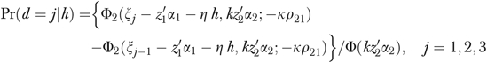(7)

where ρ₂₁ is the correlation between error terms u₁ and u₂ with pdf , and Φ and Φ₂ are the univariate and bivariate standard normal cumulative distribution functions, respectively. Define the bivariate standard normal probability as

(8)

with integration limits

(9)

Then, the category means of y conditional on no exercise (h=0) are

(10)

where

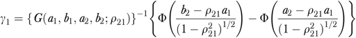(11)

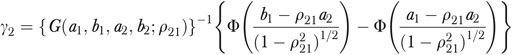(12)

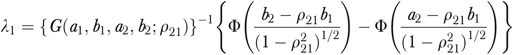(13)

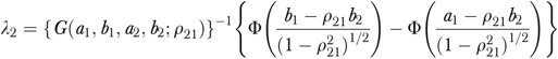(14)

The category conditional mean with exercise, that is, , is also given by (10), with an additional term δ_jh on the right-hand side and with integration limits changed slightly to and b₂=∞ in (9). The conditional mean (10) is an extension of that in Tunali (1986) and Fishe, Trost, and Lurie (1981) with dual single truncations to one with dual double truncations in the random error terms, and detailed derivations are available in S. T. Yen and J. Rosinski (unpublished data). Marginal effects of explanatory variables on the probabilities of weight categories and on BMI are calculated by differentiating (or differencing, in the case of discrete variables) the above expressions for the probabilities and conditional means. For statistical inferences, standard errors of marginal effects are calculated by the δ-method (Rao 1973, p. 388).

To evaluate the effects of exercise on BMI levels, we also calculate the average treatment effects (ATEs), which are often used in similar sample selection models (Heckman, Tobias, and Vytlacil 2001) in the program evaluation literature. Using the conditional probability (7) and conditional mean (10), the effects of exercise on the probabilities and levels of BMI for each individual of being in the jth category are, respectively,

(15)

(16)

ATEs can be calculated as the sample means of the individual effects (TE_p and TE_y) across the sample.

RESULTS

SRM Regression Estimates

Besides variables included in the other equations, healthy, cancer, and BP/heart are used solely to explain exercise, the justification being that these health belief and condition variables may affect exercise decisions more directly than they do body weight and that endogenization of exercise nevertheless allows these variables to affect body weight indirectly by way of the exercise equation. Another specification issue relates to the choice of variables for the switching equation and regression equations. Unlike two-step estimation, in which exclusion conditions are needed for identification, in maximum-likelihood estimation, the nonlinear identification criteria (i.e., linear independence of the first derivatives of the log likelihood) are met in the current system through the functional form and distributional assumptions (Buchel and van Ham 2003; Pylypchuk and Hudson 2008;). To avoid overburdening the functional form for identification, however, the system is estimated with one additional variable in the switching equation. Specifically, the squared term of age is used in the switching equation and is found significant at the 1 percent level, which suggests a nonlinear effect of age on the prevalence of overweight and obesity.

As suggested above, significant error correlations between the exercise equation and the other equations would indicate endogeneity of the former, whereas significance of the error correlations between the switching equation and the regression equations would suggest endogenous regime switching (i.e., determination of weight categories). Based on the likelihood values of the full and restricted models, LR tests suggest rejection of both the independent model (LR=108.94, df=7, p-value <.001) and the exogenous model (LR=64.25, df=4, p-value <.001).

Table 3 presents parameter estimates for the full model. The LR tests for endogeneity discussed above are confirmed by significance of the error correlations: between the switching equation and the exercise equation and between these equations and the BMI equation for the under/normal weight category.

Table 3.

Multiregime Switching Regression Estimates of BMI with Endogenous Exercise

			Regression Equations of BMI
Variable	Switching: Ordered Probit	Endogenous: Exercise	Under/Normal	Overweight	Obese
Constant	5.567	−0.058	−69.691*	76.350**	−35.810
	(13.626)	(0.112)	(37.509)	(33.975)	(153.357)
Education	−0.003	0.021***	0.019	−0.005	0.024
	(0.008)	(0.006)	(0.024)	(0.019)	(0.084)
Age	0.062***	−0.010***	0.057**	−0.044**	0.054
	(0.009)	(0.001)	(0.025)	(0.022)	(0.105)
Age2/1,000	−0.740***
	(0.045)
TV–videos	0.006	−0.055***	0.016	0.013	0.093**
	(0.006)	(0.007)	(0.017)	(0.015)	(0.045)
Income	0.056	0.099***	−0.072	−0.100	0.542
	(0.037)	(0.021)	(0.107)	(0.086)	(0.454)
City	−0.151***	−0.146***	0.028	−0.036	0.096
	(0.034)	(0.039)	(0.095)	(0.080)	(0.354)
Suburban	−0.128***	−0.149***	0.235***	0.024	−0.383
	(0.030)	(0.035)	(0.088)	(0.071)	(0.312)
Northeast	−0.008	−0.127***	0.180*	−0.046	−0.819**
	(0.040)	(0.046)	(0.108)	(0.088)	(0.423)
Midwest	0.090**	−0.034	0.167*	−0.008	−0.397
	(0.037)	(0.042)	(0.100)	(0.084)	(0.372)
South	0.019	−0.046	0.198**	0.071	−0.483
	(0.035)	(0.039)	(0.091)	(0.076)	(0.343)
White	−0.075	−0.107	0.054	−0.032	−0.108
	(0.156)	(0.073)	(0.441)	(0.366)	(1.633)
Black	0.173	−0.149*	0.051	0.072	−0.297
	(0.161)	(0.084)	(0.473)	(0.393)	(1.769)
Asian	−0.835***	−0.404***	0.006	−0.296	−2.645
	(0.182)	(0.113)	(0.451)	(0.442)	(4.572)
Hispanic	−0.065	−0.094	0.478**	0.204	−0.415
	(0.071)	(0.083)	(0.209)	(0.148)	(0.647)
Home owner	−0.036	0.031	−0.116	0.008	−0.392
	(0.030)	(0.033)	(0.082)	(0.066)	(0.296)
Professional	0.057	−0.201***	−0.641**	0.139	−0.210
	(0.104)	(0.044)	(0.290)	(0.255)	(1.158)
Manager	0.116	−0.219***	−0.568**	0.210	−0.072
	(0.104)	(0.051)	(0.292)	(0.250)	(1.090)
Farmer	0.094	−0.005	0.251	0.134	−0.747
	(0.104)	(0.119)	(0.321)	(0.191)	(1.545)
Clerical	−0.101**	−0.200***	0.181	0.000	−0.433
	(0.045)	(0.050)	(0.124)	(0.108)	(0.435)
Male	0.310***	0.377***	0.518***	−0.100	−1.383***
	(0.030)	(0.028)	(0.103)	(0.092)	(0.395)
Smoker	−0.311***	−0.114***	−0.252***	−0.027	−0.680*
	(0.028)	(0.032)	(0.080)	(0.075)	(0.364)
Vegetarian	−0.229***	0.385***	−0.903***	−0.221	−1.372
	(0.081)	(0.085)	(0.179)	(0.208)	(1.854)
Grains	−1.327		5.099*	−5.432**	11.243
	(1.086)		(2.954)	(2.644)	(11.737)
Vegetables	−0.790		5.193	−0.561	−9.756
	(1.160)		(3.326)	(2.950)	(12.175)
Fruits	0.296		0.827	0.429	−2.315
	(0.344)		(0.980)	(0.871)	(4.074)
Milk and dairy	0.458		−1.405	−1.552	12.347***
	(0.390)		(1.143)	(0.962)	(4.087)
Meat	1.518		−6.330*	5.827*	−13.167
	(1.256)		(3.412)	(3.085)	(13.923)
Fats and oils	0.066		−1.413	1.121	−2.542
	(0.482)		(1.347)	(1.187)	(5.879)
Sugar and sweets	0.288		−4.228***	1.753	−1.217
	(0.588)		(1.619)	(1.461)	(6.314)
Alc. bev.	−0.212		−0.922**	0.423	−0.943
	(0.134)		(0.388)	(0.346)	(1.451)
Nonalc. bev.	−0.941		13.085**	−7.084	13.058
	(1.981)		(5.434)	(4.904)	(22.823)
Exercise	−1.156***		2.121***	−0.239	−1.002
	(0.082)		(0.391)	(0.358)	(1.257)
Healthy		0.397***
		(0.037)
Cancer		−0.082
		(0.052)
BP/heart		−0.163***
		(0.030)
μ	0.926***
	(0.031)
σ			2.201***	1.455***	4.608***
			(0.101)	(0.036)	(0.162)
Error correlations
Exercise	0.657***
	(0.055)
Under/normal	−0.500***	−0.508***
	(0.076)	(0.090)
Overweight	−0.148	0.086
	(0.118)	(0.156)
Obese	−0.213	0.185
	(0.111)	(0.149)
Log likelihood	−34502.638

Notes: Variables income and all food quantities consumed (from grains to nonalc. bev.) are logarithmically transformed. Asymptotic standard errors in parentheses. Asterisks indicate levels of significance:

^***1%

^**5%

^*10%.

Alc. bev., alcoholic beverages; BMI, body mass index; BP, blood pressure; nonalc. bev., nonalcoholic beverages.

The exogenous and independent models, both rejected by LR tests in favor of the full model, produce notably different regression coefficients from the full model. For instance, whereas the independent model (Table 2) suggests statistical insignificance of age in the overweight equation, the full model suggests significance (at the 5 percent significance level) of age in that equation. Differences are also found in other variables such as suburban, northeast, and vegetarian.

According to parameter estimates of the full model (Table 3), age has a significant and nonlinear effect on the regime switching equation. Other significant variables in the switching equation are urbanization (city and suburban), region (midwest), race (Asian), professional category (clerical), gender (male), smoker, vegetarian, and exercise. Interestingly, none of the food intake variables is a determinant of weight categories. Over one half of the variables are significant (at the 10 percent level or lower) in the regression equation for under/normal weight, whereas significance is more scant in the regression equations for the other weight categories. Because the effects of exercise and other explanatory variables on the probabilities of weight categories and BMI level have important policy implications, we investigate the roles of these variables further by calculating ATEs and marginal effects.

Effects of Exercise

According to the ATEs presented in Table 4, exercise ameliorates overweight and obesity. Specifically, regular exercise increases the probability of being in the under/normal weight category by .04 and decreases the probabilities of overweight and obesity slightly (by .02 and .03, respectively). In terms of level, regular exercise increases BMI by 0.19 on average among individuals in the under/normal weight group while decreasing the BMI by 0.09 among individuals who are overweight.

Table 4.

Effects of Exercise on Probabilities and Levels of BMI

Category	Probability	BMI
Under/normal	0.044***	0.193***
	(0.009)	(0.070)
Overweight	−0.018***	−0.086*
	(0.003)	(0.053)
Obese	−0.026***	−0.030
	(0.007)	(0.253)

Notes: Asymptotic standard errors in parentheses. Asterisks indicate levels of significance:

^***1%

^*10%.

BMI, body mass index.

Marginal Effects of Variables

Table 5 presents the marginal effects of significant explanatory variables on the probabilities of BMI categories, conditional on exercise status and calculated at the means of all variables by exercise category. We present only the results for significant variables. The SRM produces notably different marginal effects of variables, and the rest of the analysis is based on this model. The marginal effects for many of these variables are notably different, in both signs and magnitudes, between individuals who exercise regularly and those who do not. Such differences are most often seen for the probabilities of the overweight category. For instance, whereas TV–videos increase the probability of being overweight (at the 1 percent level of significance) conditional on exercise, this variable has a negative effect on overweight conditional on no exercise (at the 10 percent level of significance). Differentiated effects on the probability of being overweight by exercise status are also seen for other variables, such as education, age, suburban, northeast, midwest, home owner, professional, clerical, healthy, and BP/heart. Echoing findings by Stettler, Signer, and Suter (2004) and Vandewater, Shim, and Caplovitz (2004) that TV, video games, and computer use contribute to childhood obesity, we find that TV–videos decrease the probability of having under/normal weight and increase the probability of being obese, both conditional and unconditional on exercise. The magnitudes of marginal effects can be very different between exercisers and nonexercisers too. For instance, vegetarians are 9.47 percent less likely to be obese than nonvegetarians conditional on exercise but 13.96 percent less likely to be obese conditional on no exercise.

Table 5.

Marginal Effects of Significant Explanatory Variables on Conditional Probabilities of BMI Categories

	Conditional on No Exercise			Conditional on Exercise
Variable	Under/Normal	Overweight	Obese	Under/Normal	Overweight	Obese
Continuous explanatory variables
Education	0.44	0.05	−0.49	0.54	−0.20*	−0.34
	(0.34)	(0.10)	(0.31)	(0.35)	(0.11)	(0.25)
Age	0.43	−0.03*	−0.40	0.06	0.01	−0.07
	(0.39)	(0.02)	(0.38)	(0.42)	(0.10)	(0.32)
TV–videos	−1.06***	−0.13*	1.19***	−1.33***	0.49***	0.83***
	(0.20)	(0.08)	(0.20)	(0.22)	(0.10)	(0.18)
Binary explanatory variables
City	3.89***	−0.38**	−3.51***	4.08***	−0.77**	−3.31***
	(1.21)	(0.18)	(1.22)	(1.36)	(0.40)	(1.00)
Suburban	2.90***	−0.35**	−2.55**	2.96***	−0.43	−2.53***
	(1.06)	(0.15)	(1.10)	(1.20)	(0.33)	(0.90)
Northeast	−1.62	−0.25	1.87	−2.13	0.92*	1.21
	(1.46)	(0.19)	(1.39)	(1.63)	(0.52)	(1.14)
Midwest	−4.16***	−0.04	4.20***	−4.73***	1.38***	3.35***
	(1.35)	(0.23)	(1.32)	(1.50)	(0.47)	(1.09)
Black	−8.46	−1.72	10.18	−10.18	1.86	8.32
	(6.27)	(0.58)	(6.47)	(7.00)	(1.69)	(5.41)
Asian	30.42***	−11.01***	−19.42***	30.30***	−14.40***	−15.90***
	(7.32)	(2.31)	(6.15)	(7.69)	(3.19)	(4.94)
Home owner	1.91*	0.07	−1.98*	2.23*	−0.68**	−1.56*
	(1.07)	(0.13)	(1.08)	(1.21)	(0.34)	(0.90)
Professional	−5.13	−0.68	5.80	−6.46	2.10**	4.36
	(3.86)	(0.48)	(4.23)	(4.51)	(0.98)	(3.58)
Manager	−7.50**	−1.12	8.62**	−9.38**	2.60	6.78*
	(3.67)	(0.78)	(4.32)	(4.37)	(0.75)	(3.74)
Clerical	1.15	−0.59***	−0.56	0.75	0.18	−0.93
	(1.63)	(0.22)	(1.50)	(1.81)	(0.63)	(1.21)
Male	−6.84***	1.03***	5.81***	−6.80***	1.16***	5.64***
	(1.06)	(0.27)	(1.08)	(1.21)	(0.45)	(0.87)
Smoker	11.25***	−1.32***	−9.93***	12.13***	−3.89***	−8.25***
	(1.08)	(0.43)	(0.96)	(1.17)	(0.56)	(0.77)
Vegetarian	17.31***	−3.35**	−13.96***	17.18***	−7.71***	−9.47***
	(3.47)	(1.58)	(2.10)	(3.23)	(1.71)	(1.65)
Healthy	5.45***	1.28***	−6.73***	7.99***	−2.60***	−5.39***
	(0.58)	(0.46)	(0.93)	(1.08)	(0.51)	(0.69)
BP/heart	−2.40***	−0.43**	2.82***	−3.19***	1.21***	1.98***
	(0.47)	(0.19)	(0.60)	(0.67)	(0.30)	(0.40)

Notes: All probabilities are multiplied by 100. Asymptotic standard errors in parentheses. Asterisks indicate levels of significance:

^***1%

^**5%

^*10%.

BMI, body mass index; BP, blood pressure.

There is more agreement qualitatively, in terms of signs and statistical significance, between the two sets of marginal effects on the probabilities for the under/normal weight and obese subgroups—conditional on no exercise and on exercise. Conditional or unconditional on regular exercise, residing in the city or a suburban area, having a clerical job, being healthy, being Asian, a home owner, a smoker, and a vegetarian all increase the probability of under/normal weights and decrease the probability of being in the obese subgroup, whereas TV–videos, residing in the midwest, having a managerial job, and being male have the opposite effects—a negative effect on the probability of having an under/normal weight and a positive effect on the probability of obesity. Interestingly, men are more likely to be overweight and obese than women, both conditional on exercise and no exercise.

Table 6 presents the marginal effects of significant explanatory variables on BMI level by exercise status. These marginal effects are also calculated at the sample means of all explanatory variables by exercise status. The model produces notably different effects of some variables on BMI from those suggested by the independent model. For instance, whereas the independent model suggests age does not affect BMI among individuals who are overweight (Table 2), the variable decreases BMI among individuals who are overweight according to the SRM. Differences are also found in other variables, such as TV–videos. Similar to their effects on probabilities of weight categories, the effects of most variables on BMI level are also similar with or without regular exercise. Exceptions are found for a few variables. For instance, conditional on exercise, grain intake decreases BMI among the overweight while alcoholic beverages and residing in the city decrease BMI among individuals with under/normal weight; these variables do not affect BMI conditional on no exercise. Home ownership decreases BMI among individuals who have under/normal weights and individuals who are obese, conditional on no exercise; this variable does not affect BMI conditional on exercise. Age is related to an increase in BMI level within the under/normal subgroup but decreases BMI within the overweight subgroup. Interestingly, TV–videos increase BMI among those overweight and obese. Some of the food intake variables affect BMI level. Specifically, grains have a negative effect and meat intake has a positive effect on BMI among individuals who are overweight, whereas milk and dairy products have a positive effect on BMI among the obese. Sugar/sweets, alcoholic beverages, and being vegetarian all decrease BMI while nonalcoholic beverages increase BMI among individuals with under/normal weight. There is some evidence of regional differences, with under/normal weight individuals from the midwest and south being heavier than their counterparts from other regions. Ethnicity is a factor, with Hispanic having a positive effect on BMI among individuals with under/normal weight. Occupations also matter. Specifically, having a professional or managerial job decreases BMI among individuals with under/normal weight. Gender differences also exist, with men in the under/normal weight category having higher BMI and men in the obese category having lower BMI than their female counterparts. Smokers consistently have lower BMI across all weight categories conditional on exercise and no exercise. Finally, conditional on exercise and no exercise, being healthy has a positive effect on BMI among individuals with under/normal weight but a negative effect on BMI among individuals who are overweight.

Table 6.

Marginal Effects of Significant Explanatory Variables on Conditional BMI Levels

	Conditional on No Exercise			Conditional on Exercise
Variable	Under/Normal	Overweight	Obese	Under/Normal	Overweight	Obese
Continuous explanatory variables
Age	0.044*	−0.046*	0.046	0.048	−0.044**	0.053
	(0.025)	(0.027)	(0.112)	(0.090)	(0.022)	(0.107)
TV–videos	0.008	0.027	0.162***	−0.013	0.026**	0.120***
	(0.014)	(0.032)	(0.043)	(0.014)	(0.013)	(0.044)
Grains	0.014	−0.020	0.032	0.014	−0.019**	0.032
	(0.010)	(0.021)	(0.042)	(0.074)	(0.008)	(0.039)
Milk and dairy	−0.005	−0.006	0.056***	−0.005	−0.006	0.054***
	(0.007)	(0.005)	(0.018)	(0.040)	(0.011)	(0.018)
Meat	−0.081	0.029**	−0.051	−0.025	0.028*	−0.052
	(0.080)	(0.015)	(0.067)	(0.081)	(0.015)	(0.064)
Sugar and sweets	−0.150***	0.069	−0.030	−0.152***	0.069	−0.035
	(0.060)	(0.055)	(0.239)	(0.060)	(0.055)	(0.240)
Alc. bev.	−0.009	0.003	−0.010	−0.007***	0.002	−0.008
	(0.007)	(0.002)	(0.013)	(0.002)	(0.003)	(0.010)
Nonalc. bev.	0.013	−0.008	0.012	0.013**	−0.008	0.012
	(0.009)	(0.006)	(0.023)	(0.006)	(0.005)	(0.025)
Binary explanatory variables
City	−0.116	−0.054	0.051	−0.141*	−0.056	−0.001
	(0.085)	(0.074)	(0.334)	(0.085)	(0.074)	(0.333)
Northeast	0.146	−0.021	−0.686*	0.100	−0.023	−0.777*
	(0.101)	(0.086)	(0.422)	(0.101)	(0.086)	(0.421)
Midwest	0.225**	0.030	−0.234	0.196**	0.027	−0.294
	(0.095)	(0.082)	(0.364)	(0.095)	(0.082)	(0.363)
South	0.201**	0.088	−0.403	0.181**	0.086	−0.447
	(0.086)	(0.076)	(0.342)	(0.085)	(0.076)	(0.341)
Hispanic	0.410**	0.203	−0.400	0.386**	0.202	−0.444
	(0.196)	(0.145)	(0.638)	(0.193)	(0.145)	(0.638)
Home owner	−0.136*	−0.011	−0.476*	−0.117	−0.010	−0.441
	(0.078)	(0.065)	(0.292)	(0.078)	(0.065)	(0.293)
Professional	−0.641**	0.200	0.088	−0.730***	0.198	−0.070
	(0.285)	(0.253)	(1.164)	(0.283)	(0.253)	(1.172)
Manager	−0.525*	0.293	0.319	−0.635**	0.293	0.139
	(0.288)	(0.250)	(1.113)	(0.285)	(0.250)	(1.121)
Male	0.830***	−0.079	−1.378***	0.912***	−0.075	−1.217***
	(0.077)	(0.063)	(0.290)	(0.078)	(0.063)	(0.294)
Smoker	−0.501***	−0.106*	−0.989***	−0.487***	−0.104*	−0.954***
	(0.072)	(0.064)	(0.303)	(0.072)	(0.064)	(0.303)
Vegetarian	−0.938***	−0.400**	−2.195	−0.808***	−0.350*	−1.696
	(0.158)	(0.196)	(1.840)	(0.158)	(0.198)	(1.845)
Healthy	0.077***	−0.080*	−0.425***	0.243***	−0.088*	−0.191***
	(0.031)	(0.049)	(0.139)	(0.078)	(0.053)	(0.069)
BP/heart	−0.035**	0.035	0.181***	−0.098***	0.033	0.067**
	(0.015)	(0.022)	(0.067)	(0.034)	(0.021)	(0.028)

Notes: Asymptotic standard errors in parentheses. Asterisks indicate levels of significance:

^***1%

^**5%

^*10%.

Alc. bev., alcoholic beverages; BMI, body mass index; BP, blood pressure; nonalc. bev., nonalcoholic beverages.

CONCLUSIONS AND DISCUSSIONS

Motivated by results of preliminary OLS analyses, we develop a multiregime SRM to investigate the differentiated roles of lifestyle, dietary, and sociodemographic variables on BMI by weight categories. We also accommodate endogeneity of an important lifestyle/behavioral variable—exercise. Weight categories and exercise are found to be endogenous. The multiregime SRM is particularly appealing because the differentiated effects of variables on BMI have important implications, and these differentiated effects would have been disguised with the use of more traditional analytical frameworks. Results suggest that sociodemographic characteristics, lifestyle, and dietary behavior affect the probabilities of individuals being in weight categories and the level of BMI. Also, these effects differ by weight category. Therefore, it is important to differentiate these effects by weight category when designing cost-effective intervention programs. They can be used to pinpoint those who are more susceptible to being overweight and obese and to target individuals for health intervention and nutritional education.

Supporting Information

Additional supporting information may be found in the online version of this article:

Appendix SA1: Author Matrix.

Appendix SA2: Development of the Likelihood Function.

Please note: Wiley-Blackwell is not responsible for the content or functionality of any supporting materials supplied by the authors. Any queries (other than missing material) should be directed to the corresponding author for the article.

REFERENCES

- Amemiya T. Advanced Econometrics. Cambridge, MA: Harvard University Press; 1985. [Google Scholar]
- Audrain JE, Klesges RC, Klesges LM. Relationship between Obesity and the Metabolic Effects of Smoking in Women. Health Psychology. 1995;14(2):116–23. doi: 10.1037//0278-6133.14.2.116. [DOI] [PubMed] [Google Scholar]
- Auld MC, Powell LM. The Economics of Obesity: Research and Policy Implications from a Canada–U.S. Comparison. In: Beach CM, Chaykowski RP, Shortt S, St-Hilaire F, Sweetman A, editors. Health Services Restructuring in Canada: New Evidence and New Directions. Kingston, Ontario: School of Policy Studies Queen's University; 2006. pp. 305–32. [Google Scholar]
- Bryant WK. Durables and Wives Employment Yet Again. Journal of Consumer Research. 1988;15(1):37–47. [Google Scholar]
- Buchel F, van Ham M. Overeducation, Regional Labor Markets, and Spatial Flexibility. Journal of Urban Economics. 2003;53(3):482–93. [Google Scholar]
- Chen Z, Meltzer DO. Beefing up with the Chans: Evidence for the Effects of Relative Income and Income Inequality on Health from the China Health and Nutrition Survey. Social Science & Medicine. 2008;66(11):2206–17. doi: 10.1016/j.socscimed.2008.01.016. [DOI] [PubMed] [Google Scholar]
- Chen Z, Yen ST, Eastwood DB. Effects of Food Stamp Participation on Body Weight and Obesity. American Journal of Agricultural Economics. 2005;87(5):1167–73. [Google Scholar]
- Chen Z, Yen ST, Eastwood DB. Does Smoking Have a Causal Effect on Weight Reduction? Journal of Family and Economic Issues. 2007;28(1):49–67. [Google Scholar]
- Chou SY, Grossman M, Saffer H. An Economic Analysis of Adult Obesity: Results from the Behavior Risk Factor Surveillance System. Journal of Health Economics. 2004;23(3):565–87. doi: 10.1016/j.jhealeco.2003.10.003. [DOI] [PubMed] [Google Scholar]
- Christiansen E, Garby L, Sørensen TIA. Quantitative Analysis of the Energy Requirements for Development of Obesity. Journal of Theoretical Biology. 2005;234(1):99–106. doi: 10.1016/j.jtbi.2004.11.012. [DOI] [PubMed] [Google Scholar]
- Costa-Font J, Gil J. Obesity and the Incidence of Chronic Diseases in Spain: A Seemingly Unrelated Probit Approach. Economics and Human Biology. 2005;3(2):188–214. doi: 10.1016/j.ehb.2005.05.004. [DOI] [PubMed] [Google Scholar]
- Cutler DM, Glaeser EL, Shapiro JM. Why Have Americans Become More Obese? Journal of Economic Perspectives. 2003;17(3):93–118. [Google Scholar]
- Fishe RPH, Trost RP, Lurie PM. Labor Force Earnings and College Choice of Young Women: An Examination of Selectivity Bias and Comparative Advantage. Economics of Education Review. 1981;1(2):169–91. [Google Scholar]
- Fox MK, Cole N. Nutrition and Health Characteristics of Low-Income Populations: Vol. 1, Food Stamp Program Participants and Nonparticipants, E-FAN-04-014-1. Washington, DC: United States Department of Agriculture, Economic Research Service; 2004. [Google Scholar]
- Heckman J, Tobias JL, Vytlacil E. Four Parameters of Interest in the Evaluation of Social Programs. Southern Economic Journal. 2001;68(2):210–23. [Google Scholar]
- Huffman SK, Rizov M. Determinants of Obesity in Transition Economies: The Case of Russia. Economics and Human Biology. 2007;5(3):379–91. doi: 10.1016/j.ehb.2007.07.001. [DOI] [PubMed] [Google Scholar]
- Jensen TK, Andersson AM, Jorgensen N, Andersen AG, Carlsen E, Petersen JO, Skakkebaek NE. Body Mass Index in Relation to Semen Quality and Reproductive Hormones among 1,558 Danish Men. Fertility and Sterility. 2004;82(4):863–70. doi: 10.1016/j.fertnstert.2004.03.056. [DOI] [PubMed] [Google Scholar]
- Kan K, Tsai W. Obesity and Risk Knowledge. Journal of Health Economics. 2004;23(5):907–34. doi: 10.1016/j.jhealeco.2003.12.006. [DOI] [PubMed] [Google Scholar]
- Kim SY, Nayga RM, Jr., Capps O., Jr The Effect of Food Label Use on Nutrient Intakes: An Endogenous Switching Regression Analysis. Journal of Agricultural and Resource Economics. 2000;25(1):215–31. [Google Scholar]
- Kuchler F, Variyam JN. Mistakes Were Made: Misperception as a Barrier to Reducing Overweight. International Journal of Obesity. 2003;27(7):856–61. doi: 10.1038/sj.ijo.0802293. [DOI] [PubMed] [Google Scholar]
- Lakdawalla D, Philipson TJ. The Growth of Obesity and Technological Change: A Theoretical and Empirical Examination. NBER Working Paper # 8946.
- Lin BH, Huang CL, French SA. Factors Associated with Women's and Children's Body Mass Indices by Income Status. International Journal of Obesity. 2004;28(4):536–42. doi: 10.1038/sj.ijo.0802604. [DOI] [PubMed] [Google Scholar]
- McKelvey RD, Zavoina W. A Statistical Model for the Analysis of Ordinal Level Dependent Variables. Journal of Mathematical Sociology. 1975;4:103–20. [Google Scholar]
- Mokdad AH, Ford ES, Bowman BA, Dietz WH, Vinicor F, Bales VS, Marks JS. Prevalence of Obesity, Diabetes, and Obesity-Related Health Risk Factors, 2001. Journal of the American Medical Association. 2003;289(1):76–9. doi: 10.1001/jama.289.1.76. [DOI] [PubMed] [Google Scholar]
- Mokdad AH, Marks JS, Stroup DF, Gerberding JL. Correction: Actual Causes of Death in the United States, 2000. Journal of the American Medical Association. 2005;293(3):293–4. doi: 10.1001/jama.293.3.293. [DOI] [PubMed] [Google Scholar]
- National Institutes of Health (NIH) Clinical Guidelines on the Identification, Evaluation and Treatment of Overweight and Obesity in Adults: The Evidence Report. Obesity Research. 1998;6(suppl 2):51S–209S. [PubMed] [Google Scholar]
- Nayga RM. Schooling, Health Knowledge and Obesity. Applied Economics. 2000;32(7):815–22. [Google Scholar]
- Ogden CL, Flegal KM, Carroll MD, Johnson CL. Prevalence and Trends in Overweight among US Children and Adolescents, 1999–2000. Journal of the American Medical Association. 2002;288(14):1728–32. doi: 10.1001/jama.288.14.1728. [DOI] [PubMed] [Google Scholar]
- Philipson TJ, Posner RA. The Long-Run Growth in Obesity as a Function of Technological Change. NBER Working Paper # 7423. [PubMed]
- Poirier DJ. The Use of the Box-Cox Transformation in Limited Dependent Variable Models. Journal of American Statistical Association. 1978;73(362):284–7. [Google Scholar]
- Pylypchuk Y, Hudson J. Immigrants and the Use of Preventive Care in the United States. Health Economics. 2008 doi: 10.1002/hec.1401. published online. doi 10.1002/hec.1401. [DOI] [PubMed] [Google Scholar]
- Rao CR. Linear Statistical Inference and Its Applications. 2d Edition. New York: John Wiley & Sons; 1973. [Google Scholar]
- Roy AD. Some Thoughts on the Distribution of Earnings. Oxford Economic Papers. 1951;3(2):135–46. [Google Scholar]
- Schroeter C, Lusk J, Tyner W. Determining the Impact of Food Price and Income Changes on Body Weight. Journal of Health Economics. 2008;27(1):45–68. doi: 10.1016/j.jhealeco.2007.04.001. [DOI] [PubMed] [Google Scholar]
- Stettler N, Signer TM, Suter PM. Electronic Games and Environmental Factors Associated with Childhood Obesity in Switzerland. Obesity. 2004;12(6):896–903. doi: 10.1038/oby.2004.109. [DOI] [PubMed] [Google Scholar]
- Stunkard AJ, Wadden TA, editors. Obesity: Theory and Therapy. 2d Edition. New York: Raven Press; 1993. [Google Scholar]
- Tunali I. A General Structure for Models of Double-Selection and an Application to a Joint Migration-Earnings Process with Remigration. Research in Labor Economics. 1986;8(B):235–84. [Google Scholar]
- U.S. Department of Agriculture, Agricultural Research Service (USDA-ARS) Continuing Survey of Food Intakes by Individuals 1994–96, CD-ROM. Washington, DC: U.S. Department of Agriculture, Agricultural Research Service (USDA-ARS); 2000. [Google Scholar]
- U.S. Department of Health and Human Services (USDHHS) Healthy People 2010: Volume I and II. 2d Edition. Washington, DC: U.S. Government Printing Office; 2000. [Google Scholar]
- U.S. Department of Health and Human Services (USDHHS) The Surgeon General's Call to Action to Prevent and Decrease Overweight and Obesity. Rockville, MD: U.S. Department of Health and Human Services, Public Health Service, Office of the Surgeon General; 2001. [PubMed] [Google Scholar]
- Vandewater EA, Shim M, Caplovitz AG. Linking Obesity and Activity Level with Children's Television and Video Game Use. Journal of Adolescence. 2004;27(1):71–85. doi: 10.1016/j.adolescence.2003.10.003. [DOI] [PubMed] [Google Scholar]
- Ver Ploeg M, Mancino L, Lin B, Wang C. The Vanishing Weight Gap: Trends in Obesity among Adult Food Stamp Participants (US) (1976–2002) Economics and Human Biology. 2007;5(1):20–36. doi: 10.1016/j.ehb.2006.10.002. [DOI] [PubMed] [Google Scholar]
- Vijverberg WPM. Measuring the Unidentified Parameter of the Extended Roy Model of Selectivity. Journal of Econometrics. 1993;57(1–3):69–89. [Google Scholar]
- Wilde EP, Ranney CK. The Monthly Food Stamp Cycle: Shopping Frequency and Food Intake Decisions in an Endogenous Switching Regression Framework. American Journal of Agricultural Economics. 2000;82(1):200–13. [Google Scholar]
- World Health Organization. Obesity: Preventing and Managing the Global Epidemic. Report of a WHO Consultation on Obesity. Geneva, Switzerland: Work Health Organization; 1998. [PubMed] [Google Scholar]
- Yen ST. Working Wives and Food Away from Home: The Box-Cox Double Hurdle Model. American Journal of Agricultural Economics. 1993;75(4):884–95. [Google Scholar]
Associated Data
This section collects any data citations, data availability statements, or supplementary materials included in this article.