Improving sensitivity in micro-free flow electrophoresis using signal averaging

Abstract

Microfluidic free-flow electrophoresis (μFFE) is a separation technique that separates continuous streams of analytes as they travel through an electric field in a planar flow channel. The continuous nature of the μFFE separation suggests that approaches more commonly applied in spectroscopy and imaging may be effective in improving sensitivity. The current paper describes the S/N improvements that can be achieved by simply averaging multiple images of a μFFE separation; 20–24-fold improvements in S/N were observed by averaging the signal from 500 images recorded for over 2 min. Up to an 80-fold improvement in S/N was observed by averaging 6500 images. Detection limits as low as 14 pM were achieved for fluorescein, which is impressive considering the non-ideal optical set-up used in these experiments. The limitation to this signal averaging approach was the stability of the μFFE separation. At separation times longer than 20 min bubbles began to form at the electrodes, which disrupted the flow profile through the device, giving rise to erratic peak positions.

1 Introduction

Free-flow electrophoresis (FFE) is an established technique that has been used to separate samples ranging from proteins, [1–3] to whole cells, [4, 5] to cellular components. [6–10] Separations are performed in a planar flow channel. To achieve a separation a voltage is applied perpendicularly to the pressure-driven flow in the channel, deflecting analyte streams laterally according to their mobility in the electric field. Analyte streams are detected in the flow channel or, as is more common, collected as fractions.

Raymond et al. were the first to miniaturize FFE in a silicon/glass device [11]. Performing FFE in a microfluidic format (μFFE) reduces sample and buffer volume requirements, simplifies flow profiles, and improves heat dissipation [12]. More recently μFFE devices have been fabricated in PDMS [13] and all glass substrates [14]. Early devices suffered from the generation of electrolysis products at the electrodes but a number of approaches have been introduced to reduce bubble formation including multiple depth designs [15], isolation by ion permeable membranes [16], and the use of capacitive electrodes [17]. These improvements have yielded devices that have been successfully applied to a number of analytes including fluorescent dyes [13, 15, 16], fluorescently labeled amino acids [11], and fluorescently labeled proteins [18, 19]. A theory has been developed to describe the effect of parameters such as flow rate and electric field on band broadening and resolution in μFFE [20]. Applications that take advantage of the unique characteristics of μFFE separations such as isoelectric focusing [16, 21] and gradient μFFE [22] are beginning to be explored.

Since the earliest introduction of microfluidic separations, sensitivity has been identified as a potential limitation [23]. Small masses and volumes of analyte combined with short path lengths challenged existing detector technology. Since then elaborate LIF detector arrangements such as the sheath flow cuvette have been employed to improve sensitivity in CE [24]. Size and shape constraints of microfluidic chips prevent the application of some of these arrangements but low picomolar detection limits have been achieved using LIF detection in confocal [25, 26] and non-confocal [27–29] arrangements.

More numerical approaches have also been applied to improve S/N in CE. Culbertson and Jorgenson used a diode array detector to generate multiple UV absorbance signals from a single separation [30, 31]. S/N was improved by up to 35-fold when these signals were averaged. Kaneta et al. injected a pseudo-random pulse sequence onto a capillary [32]. A Hadamard transform was used to deconvolute and average the data set into an individual electropherogram. This approach improved S/N 18-fold over a traditional CE injection [33]. More recently, Hadamard transforms have been used to improve S/N eightfold in a microfluidic device [34].

At first it might seem that detection limits in μFFE would be expected to be even poorer than those of CE separations performed in microfluidic chips. All of the size and dimensional constraints of microfluidic chips remain preventing optimal LIF detector arrangements from being employed. In addition, an approximately 1 cm area across the exit of the separation channel must be imaged to detect the position of the deflected analyte streams. This requirement of a large field of view prevents the use of high numerical aperture objectives for efficient collection of fluorescence photons. Images must be recorded using CCD cameras, not the high-sensitivity PMTs commonly used in CE-LIF detectors. Lastly, the source light for fluorescence excitation must be extended across the outlet of the separation channel.

Balancing the detection drawbacks of μFFE is the continuous nature of the separation. In a traditional separation, the signal for a peak must be recorded as the analyte races past the detector. Over a 15 minute separation, the time used to quantitate an analyte may be seconds or less. This is not an efficient use of detector time. Averaging multiple separations is not practical due to the reproducibility required between separations and the time required to perform multiple analyses. In contrast, a μFFE separation presents a static image that can be observed over long periods of time. A large number of images can be collected in a relatively short period of time, presenting an opportunity for signal averaging not practical in conventional separations. This is analogous to high-sensitivity fluorescence [35, 36], radioactivity [37], and chemiluminescence [38] detection that is possible in traditional slab gel electrophoresis, which also presents a static separation that can be imaged over long periods of time. The current paper investigates the S/N improvements that can be achieved in μFFE using this strategy.

2 Materials and methods

2.1 Reagents and chemicals

Unless otherwise noted all chemicals were purchased from Sigma-Aldrich (St. Louis, MO). Deionized water (18.3 MΩ, Barnstead, Dubuque, IA) was used for all preparations unless otherwise noted. A 25 mM HEPES separation buffer was prepared and adjusted to pH=7.00 using 1 M NaOH and filtered through a 0.2 μm membrane filter (Fisher Scientific, Fairlawn, NJ). Stock solutions of disodium fluorescein (Acros, NJ), Rhodamine 123 chloride and Rhodamine 110 were prepared in 190 proof Ethanol (Fisher Scientific) and serial diluted with separation buffer. Piranha solutions (4:1 H₂SO₄:H₂O₂, Ashland Chemical, Dublin, OH) were used to clean glass wafers and etch deposited Ti. Aqua regia (3:1 HCl:HNO₃, Ashland Chemical) was used to etch Pd. Concentrated HF (Ashland Chemical) was used to etch the glass wafers. Silver conductive epoxy (MG Chemicals, Surrey, B.C., Canada) was used to make electrical connections to the electrodes on the μFFE device.

2.2 Chip fabrication

A μFFE device was fabricated using a two-step etch method to create a multiple depth design as previously described [22]. Briefly, standard photolithography techniques were used to etch 57 μm deep electrode channels into a 1.1 mm borofloat wafer (Precision Glass & Optics, Santa Ana, CA). A second etch step defined the remaining features of the chip. The final depths of the electrode and separation channels were 73 and 19 μm, respectively. Titanium (100 nm), palladium (100 nm), and chromium (100 nm) layers were deposited followed by a third photolithography procedure to define the electrodes. Chromium etchant CR-12 was used to remove Cr mask and Aqua regia and Piranha were used to etch Pd and Ti, respectively. A second wafer was predrilled with access holes and deposited with an ∼90 nm thick layer of amorphous silicon. The etched wafer was aligned with the drilled wafer and anodically bonded (900 V, 2 h, 450°C, and 5 μbar). Nanoports (Upchurch Scientific, Oak Harbor, WA) were attached to the access holes using manufacturer's procedures. Silver conductive epoxy was pushed into electrode access holes and used to secure silver wires. The chip was perfused with 1 M NaOH until the channels were clear of unwanted amorphous silicon.

2.3 μFFE separations

A syringe pump (Harvard Apparatus) was used to pump separation buffer into the chip at 0.375 mL/min (0.10 cm/s in the separation channel). Dye mixtures were pumped into the sample channel at 50.0 nL/min (0.12 cm/s in the sample channel). A separation voltage of 50 V was applied at the right electrode.

2.4 μFFE instrumentation, data collection, and processing

Images were acquired using a Cascade 512B CCD camera (Photometrics, Tucson, AZ) attached to a SMZ 1500 stereomicroscope (Nikon, Tokyo, Japan). The chip was positioned to focus the microscope (0.75 × zoom) ∼1.5 cm downstream from the sample inlet. A 50 mW, 488 nm solid state laser (Newport, Irvine, CA) was expanded to an ∼2.5 cm wide by ∼150 μm thick line across the separation channel of the chip directly below the microscope objective. The chip, microscope, optics, and laser were all enclosed using black rubberized fabric (Thorlabs, Newton, NJ). The microscope was equipped with an Endow GFP bandpass emission filter cube (Nikon) containing two bandpass filters (450–490 and 500–550 nm) and a dichroic mirror (495 nm cutoff). A 1.6 × objective was used for collection with a 0.7 × CCD camera lens. MetaVue software (Downington, PA) was used for image collection and linescan processing across analyte stream. Images were acquired consecutively with an exposure time of 100 ms and 4095 intensifier gain. Linescans with a width of one pixel were extracted from the images with no filtering. Signals were averaged after background subtraction utilizing a custom-made LabView program. Analysis of the averaged linescans was performed using Cutter 5.0 [39].

3 Results and discussion

Figure 1A shows an image of a μFFE separation of three fluorescent dyes recorded near their LOD. As expected, the dyes are deflected in the electric field according to their mobility. The electroosmotic flow enhances the mobility of rhodamine 123, increasing the deflection of this analyte stream. Similarly, the electroosmotic flow counters the negative electrophoretic mobility of fluorescein, resulting in minimal deflection of this analyte.

Figure 1.

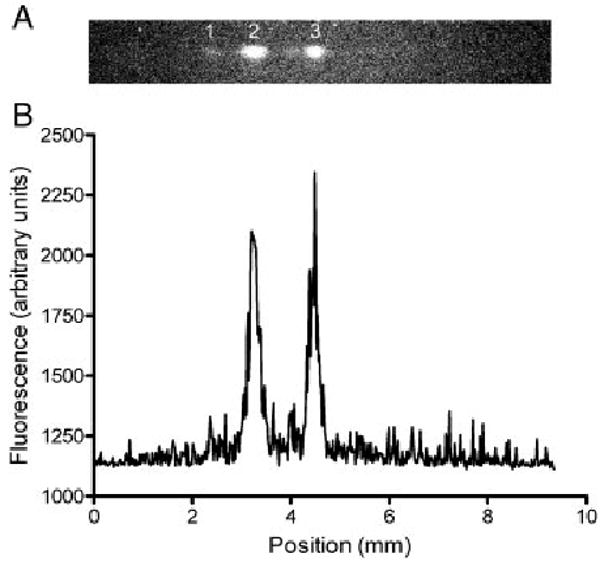
(A) Image of a μFFE separation of rhodamine 123 (1), rhodamine 110 (2), and fluorescein (3). (B) A linescan of the same μFFE separation. The separation voltage was 50 V (anode on the right) and the buffer flow rate was 0.375 mL/min. The concentration of all analytes was 10 nM.

Figure 1B is a linescan across the μFFE image, giving data analogous to an electropherogram. Clearly, the S/N is low and the analytes are near the LOD. A common strategy for improving LOD in spectroscopy or imaging applications is to increase the number of measurements (n) with S/N increasing proportionally to n^1/2. This approach is often not practical in separation techniques due to the time required to collect an individual chromatogram or electropherogram and the level of reproducibility between separations necessary for signal averaging to be effective. μFFE is not limited in this way. The single image shown in Fig. 2 was recorded in 100 ms. Using this exposure time an image of the separation can be recorded every 240 ms. This timescale is much more amenable to signal averaging large numbers of images. Being able to record a large number of images in a short period of time also makes it easier to achieve the reproducibility in peak position necessary for signal averaging to be effective.

Figure 2.

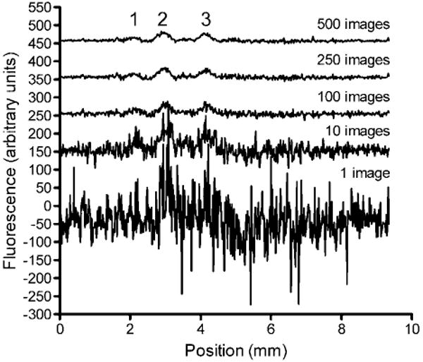
Effect of averaging multiple linescans on S/N in a μFFE separation of 2 nM rhodamine 123 (1), 500 pM rhodamine 110 (2), and 500 pM fluorescein (3). The exposure time for a single image was 100 ms. The time between subsequent images was 240 ms. Linescans have been offset for clarity.

Figure 2 shows a series of linescans where 1–500 images have been signal averaged. Clearly, signal averaging significantly improves the S/N of the peaks. Peaks that are barely distinguishable from noise are distinctly observable when 500 images are averaged. Considering the 240 ms required to acquire a single image, 500 images can be recorded in 2 min. This is faster than the typical time required to perform a single CE or chromatography separation. Similar results were obtained by collecting a single image with a long exposure time (data not shown). Averaging many images with short exposure times is preferred because it avoids detector saturation that can occur at very long exposure times.

Figure 3A compares the number of images averaged with the observed improvement in S/N observed for each analyte. Over short periods of time (i.e. 1000 images, 4 min recording time) the curves closely resemble the theoretical S/N∝n^1/2 limit. Averaging 500 images (2 min recording time) resulted in a 20–24-fold improvement in S/N over a single image, which closely matches the theoretical 22.4-fold improvement. Even averaging 10 images (2.4 s recording time) resulted in a fourfold improvement in S/N.

Figure 3.

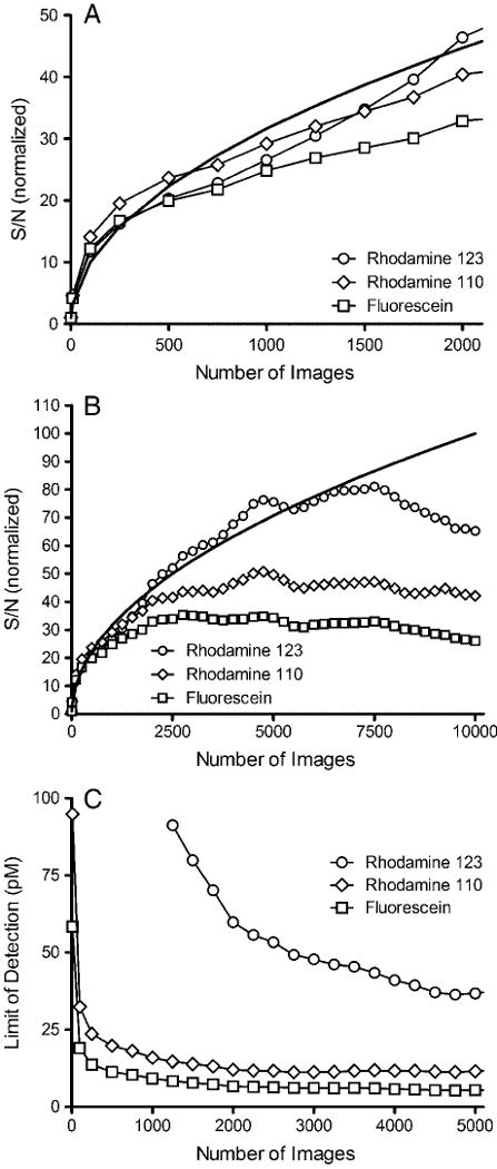
Effect of number of images averaged on the improvement in S/N (A and B) and LOD (C) in a μFFE separation of 2 nM rhodamine 123 (circles), 500 pM rhodamine 110 (diamonds), and 500 pM fluorescein (squares). The data in (A) and (B) have been normalized to the S/N observed in a single image for each analyte. The solid lines in (A) and (B) show the theoretical curves where S/N is proportional to n^1/2.

The effectiveness of signal averaging is ultimately limited by the reproducibility of peak position in repeated images. If the peak position changes between images, broadening and decreased peak height result, effectively eliminating any gains in S/N. Figure 4A shows a stack of 1000 μFFE separations. Peak position is relatively stable over this 4 min time period. This correlates well with the improvement in S/N observed in Fig. 3A. Figure 4B illustrates peak position over 10 000 images (40 min recording time). Peak position is stable up to ∼5000 images (20 min recording time). Beyond this point, peak position becomes erratic. This variation in peak position is likely due to bubble formation over long periods of voltage application. As shown in Fig. 3B, the variation in peak position limits S/N improvements when images are recorded over long periods of time (i.e. >2000 images).

Figure 4.

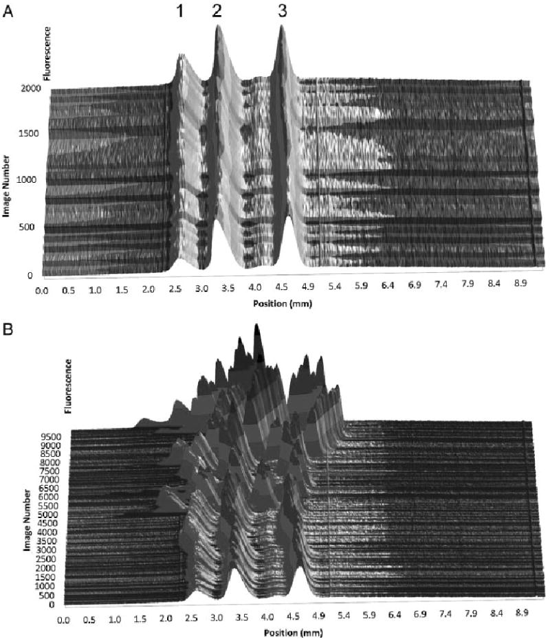
A stacked plot of linescans demonstrating peak position stability over time of a μFFE separation of 50 nM rhodamine 123 (1), rhodamine 110 (2), and fluorescein (3). Sets of 50 subsequent linescans were grouped and averaged before they were plotted to improve S/N. As shown in (A) peak position is stable up to approximately 2000 images (8 min collection time). Over the longer separation times shown in (B) peak position becomes erratic due to formation of electrolysis products at the electrodes.

It should be noted that the improvement in S/N plateaued at different times for each analyte. Rhodamine 123 closely follows the theoretical curve up to 6500 images resulting in an 80-fold improvement in S/N. Rhodamine 110 follows the theoretical curve up to 2000 images before leveling off at a S/N improvement of 45. Fluorescein begins to deviate from the theoretical curve at 500 images before plateauing at 2000 images (S/N improvement of 35). This trend matches the migration distances of the analytes with rodamine 123 being deflected the most and fluorescein the least. Migration distance is a significant contributor to band broadening in μFFE [20]. Analyte streams that are deflected most are the broadest. This is true in the current separations where rhodamine 123 is the broadest peak followed by rhodamine 110 and fluorescein (see Fig. 5). Taking this into consideration it is not surprising that variations in peak position affect fluorescein first. If the bandwidth is narrow, small variations in peak position move the band off of the original image, broadening the peak and negating any benefit from signal averaging. This is confirmed in Fig. 5 where the band for fluorescein exhibits the largest increase in peak width as the separation becomes unstable at recording times greater than 2500 images. Broader bands are more forgiving since the original and shifted peaks may still partially overlap. Again this is confirmed in Fig. 5 where the peak width of rhodamine 123 is not affected as much as that of fluorescein as peak position becomes less stable.

Figure 5.

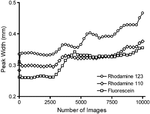
Effect of number of images averaged on peak width in a μFFE separation of rhodamine 123 (circles), rhodamine 110 (diamonds), and fluorescein (squares).

While it is clear that signal averaging is beneficial in improving the concentration LOD, as shown in Fig. 6 there is a trade-off in the mass LOD (MLOD). As described above S/N increases at the theoretical rate proportional to n^1/2 as long as peak position remains stable. Unfortunately the volume, and therefore mass, of analyte introduced into the device is directly proportional to time. The result is that the MLOD increases proportionally to n^1/2. This trend can be observed in Fig. 6A. At higher numbers of images the S/N plateaus as peak position becomes less stable and the MLOD increases linearly (see Fig. 6B). The result is that MLOD of μFFE is much poorer than CE even though similar concentration of LODs can be obtained through signal averaging.

Figure 6.

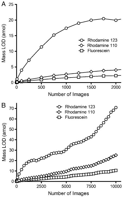
Effect of number of images averaged over periods of 8 minutes (A) and 40 minutes (B) on the mass limit of detection (MLOD) in a μFFE separation of 2 nM rhodamine 123 (circles), 500 pM rhodamine 110 (diamonds) and 500 pM fluorescein (squares).

4 Concluding remarks

The signal measured in μFFE is inherently different than those of more commonly encountered separation techniques. Traditional separations such as chromatography and electrophoresis separate analytes in time. Signal is therefore recorded over time as analytes exit the column. The result is that the detector often spends most of the time measuring the signal between peaks (i.e. baseline). In μFFE analytes are separated in space. If the sample entering the device does not change, a static image is recorded. This opens the door to S/N improvement strategies more commonly applied in spectroscopy and imaging applications. Signal averaging is an excellent example of this. In the current manuscript 20–24-fold improvements in S/N were observed by averaging the signal from 500 images recorded over 2 min; this improved LODs for fluorescein from 500 to 14 pM, rhodamine 110 from 500 to 11 pM and rhodamine 123 from 2 nM to 25 pM. These are impressive concentration LODs considering detection was performed using a simple fluorescence microscope with a relatively low numerical aperture objective (0.21) combined with on-chip LIF operated in a non-confocal arrangement.

The current limitation of signal averaging in μFFE is variation in peak position. S/N generally improved up to 2000 images (8 min collection time). Further improvements in μFFE design to reduce the effect of bubbles generated by electrolysis over long time periods could make signal averaging over even longer periods possible. It should be noted that diminishing improvements in S/N are observed with longer times due to the S/N∝n^1/2 relationship. At some point the improvement in S/N will not justify the time required to collect images. Averaging 500–2000 images, generating a 20–45-fold S/N improvement in 2–8 min would seem to be a good trade-off between sensitivity, time, and peak stability.

Abbreviations

FFE

free-flow electrophoresis

MLOD

mass LOD

μFFE

microfluidic FFE

References

- 1.Wang Y, Hancock WS, Weber G, Eckerskorn C, Palmer-Toy D. J Chromatogr A. 2004;1053:269–278. [PubMed] [Google Scholar]
- 2.Zischka H, Weber G, Weber PJA, Posch A, Braun RJ, Buehringer D, Schneider U, et al. Proteomics. 2003;3:906–916. doi: 10.1002/pmic.200300376. [DOI] [PubMed] [Google Scholar]
- 3.Moller E, Greaves MF, Zuo X, Lee K, Speicher DW. In: Proteome Anal: Interpreting the Genome. Speicher DW, editor. Elsevier; New York: 2004. pp. 93–118. [Google Scholar]
- 4.Graham JM, Wilson RBJ, Patel K. Methodol Surv Biochem Anal. 1987;17:143–152. [Google Scholar]
- 5.Heidrich HG, Hannig K. Methods Enzymol. 1989;171:513–531. doi: 10.1016/s0076-6879(89)71028-4. [DOI] [PubMed] [Google Scholar]
- 6.Hoffstetter-Kuhn S, Kuhn R, Wagner H. Electrophoresis. 1990;11:304–309. doi: 10.1002/elps.1150110406. [DOI] [PubMed] [Google Scholar]
- 7.Hoffstetter-Kuhn S, Wagner H. Electrophoresis. 1990;11:451–456. doi: 10.1002/elps.1150110603. [DOI] [PubMed] [Google Scholar]
- 8.Hoffstetter-Kuhn S, Wagner H. Electrophoresis. 1990;11:457–462. doi: 10.1002/elps.1150110604. [DOI] [PubMed] [Google Scholar]
- 9.Kessler R, Manz HJ. Electrophoresis. 1990;11:979–980. doi: 10.1002/elps.1150111119. [DOI] [PubMed] [Google Scholar]
- 10.Poggel M, Melin T. Electrophoresis. 2001;22:1008–1015. doi: 10.1002/1522-2683()22:6<1008::AID-ELPS1008>3.0.CO;2-A. [DOI] [PubMed] [Google Scholar]
- 11.Raymond DE, Manz A, Widmer HM. Anal Chem. 1994;66:2858–2865. [Google Scholar]
- 12.Kohlheyer D, Eijkel JCT, van den Berg A, Schasfoort RBM. Electrophoresis. 2008;29:977–993. doi: 10.1002/elps.200700725. [DOI] [PubMed] [Google Scholar]
- 13.Zhang CX, Manz A. Anal Chem. 2003;75:5759–5766. doi: 10.1021/ac0345190. [DOI] [PubMed] [Google Scholar]
- 14.Fonslow BR, Bowser MT. Anal Chem. 2005;77:5706–5710. doi: 10.1021/ac050766n. [DOI] [PubMed] [Google Scholar]
- 15.Fonslow BR, Barocas VH, Bowser MT. Anal Chem. 2006;78:5369–5374. doi: 10.1021/ac060290n. [DOI] [PubMed] [Google Scholar]
- 16.Kohlheyer D, Besselink GAJ, Schlautmann S, Schasfoort RBM. Lab Chip. 2006;6:374–380. doi: 10.1039/b514731j. [DOI] [PubMed] [Google Scholar]
- 17.Janasek D, Schilling M, Manz A, Franzke J. Lab Chip. 2006;6:710–713. doi: 10.1039/b602815b. [DOI] [PubMed] [Google Scholar]
- 18.Kobayashi H, Shimamura K, Akaida T, Sakano K, Tajima N, Funazaki J, Suzuki H, Shinohara E. J Chromatogr A. 2003;990:169–178. doi: 10.1016/s0021-9673(02)01964-7. [DOI] [PubMed] [Google Scholar]
- 19.Raymond DE, Manz A, Widmer HM. Anal Chem. 1996;68:2515–2522. doi: 10.1021/ac950766v. [DOI] [PubMed] [Google Scholar]
- 20.Fonslow BR, Bowser MT. Anal Chem. 2006;78:8236–8244. doi: 10.1021/ac0609778. [DOI] [PubMed] [Google Scholar]
- 21.Kohlheyer D, Eijkel JCT, Schlautmann S, van den Berg A, Schasfoort RBM. Anal Chem. 2007;79:8190–8198. doi: 10.1021/ac071419b. [DOI] [PubMed] [Google Scholar]
- 22.Fonslow BR, Bowser MT. Anal Chem. 2008;80:3182–3189. doi: 10.1021/ac702367m. [DOI] [PMC free article] [PubMed] [Google Scholar]
- 23.Jorgenson JW, Lukacs KD. Science. 1983;222:266–272. doi: 10.1126/science.6623076. [DOI] [PubMed] [Google Scholar]
- 24.Chen DY, Dovichi NJ. Anal Chem. 1996;68:690–696. [Google Scholar]
- 25.Fister JC, Jacobson SC, Davis LM, Ramsey MJ. Anal Chem. 1998;70:431–437. doi: 10.1021/ac9707242. [DOI] [PubMed] [Google Scholar]
- 26.Ocvirk G, Tang T, Harrison J. Analyst. 1998;123:1429–1434. [Google Scholar]
- 27.Fang Q, Xu GM, Fang ZL. Anal Chem. 2002;74:1223–1231. doi: 10.1021/ac010925c. [DOI] [PubMed] [Google Scholar]
- 28.Fu JL, Fang Q, Zhang T, Jin XH, Fang ZL. Anal Chem. 2006;78:3827–3834. doi: 10.1021/ac060153q. [DOI] [PubMed] [Google Scholar]
- 29.Sanders JC, Huang Z, Landers JP. Lab Chip. 2001;1:167–172. doi: 10.1039/b107835f. [DOI] [PubMed] [Google Scholar]
- 30.Culbertson CT, Jorgenson JW. Anal Chem. 1998;70:2629–2638. doi: 10.1021/ac970654z. [DOI] [PubMed] [Google Scholar]
- 31.Culbertson CT, Jorgenson JW. J Microcholumn Sep. 1999;11:652–662. [Google Scholar]
- 32.Kaneta T, Yamaguchi Y, Imasaka T. Anal Chem. 1999;71:5444–5446. doi: 10.1021/ac990625j. [DOI] [PubMed] [Google Scholar]
- 33.Kaneta T, Kosai K, Imasaka T. Anal Chem. 2002;74:2257–2260. doi: 10.1021/ac011149b. [DOI] [PubMed] [Google Scholar]
- 34.McReynolds JA, Shippy SA. Anal Chem. 2004;76:3214–3221. doi: 10.1021/ac035404z. [DOI] [PubMed] [Google Scholar]
- 35.Miura K. Electrophoresis. 2001;22:801–813. doi: 10.1002/1522-2683()22:5<801::AID-ELPS801>3.0.CO;2-X. [DOI] [PubMed] [Google Scholar]
- 36.Weidekamm E, Wallach DFH, Flückiger R. Anal Biochem. 1973;54:102–114. doi: 10.1016/0003-2697(73)90252-2. [DOI] [PubMed] [Google Scholar]
- 37.Roberts PL. Anal Biochem. 1985;147:521–524. doi: 10.1016/0003-2697(85)90308-2. [DOI] [PubMed] [Google Scholar]
- 38.Zhang X, Ouyang J, Baeyens WRG, Delanghe JR, Dai Z, Shen S, Huang G. Anal Chim Acta. 2003;497:83–92. [Google Scholar]
- 39.Shackman JG, Watson CJ, Kennedy RT. J Chromatogr A. 2004;1040:273–282. doi: 10.1016/j.chroma.2004.04.004. [DOI] [PubMed] [Google Scholar]