Micro free-flow electrophoresis: theory and applications

Abstract

Free-flow electrophoresis (FFE) is a technique that performs an electrophoretic separation on a continuous stream of analyte as it flows through a planar flow channel. The electric field is applied perpendicularly to the flow to deflect analytes laterally according to their mobility as they flow through the separation channel. Miniaturization of FFE (μFFE) over the past 15 years has allowed analytical and preparative separation of small volume samples. Advances in chip design have improved separations by reducing interference from bubbles generated by electrolysis. Mechanisms of band broadening have been examined theoretically and experimentally to improve resolution in μFFE. Separations using various modes such as zone electrophoresis, isoelectric focusing, isotachophoresis, and field-step electrophoresis have been demonstrated.

Introduction

Electrophoresis is commonly used in biochemistry because of its ability to separate biomolecules such as proteins [1], peptides, DNA [2], and cells [3]. Common techniques such as gel electrophoresis and capillary electrophoresis (CE) are preferred because of their ability to separate biological molecules in a relatively short time without losing the functionality of the molecules. Both techniques rely on an applied electric field to separate molecules on the basis of size and charge as the molecules travel parallel to the electric field. Another less known electrophoresis technique, free-flow electrophoresis (FFE), has been developed and used for almost fifty years [4, 5]. In FFE, pressure is used to drive a sample stream though a planar separation channel (Fig. 1). An electric field is applied perpendicularly to the direction of flow to deflect analytes into distinct streams [6]. Unlike CE, sample injection, separation, and collection can take place continuously because the direction of the separation is different from that of the bulk flow. The continuous nature of the technique provides a high-throughput separation mechanism, making FFE a useful technique for preparative separations of peptides [7], cells [8, 9], cellular components [10], enzymes [11, 12], and proteins [13–15]. Various commercial instruments are available for preparative FFE. Various modes of electrophoresis, for example zone electrophoresis (ZE), isoelectric focusing (IEF), isotachophoresis (ITP), and field-step have been demonstrated using FFE [6, 16].

Fig. 1.

Illustration of separation principles. (a) A separation in capillary electrophoresis. Analytes move through the capillary according to their electrophoretic mobility and electroosmotic flow. (b) A separation in free-flow electrophoresis. Analytes move down the chip by pressure driven buffer flow. Analytes are deflected in sample streams based on their electrophoretic mobility

Although useful for preparative separations, FFE is limited by Joule heating because of the relatively large cross-sectional area and low surface area-to-volume ratios of the separation channel. In addition, resolution in FFE is complicated by a number of broadening mechanisms. In an open tube electroosmotic flow (EOF) generates a flat flow profile. In FFE electrodes are isolated from the separation region by a membrane to prevent electrolysis bubbles from disrupting the sample streams. This creates a closed system which causes electrodynamic distortion [17]. In a closed system, a counter flow is generated in the center of the channel since there is no path for the EOF to exit the channel. This counter flow gives rise to a crescent-shaped flow profile [18]. The parabolic flow profile generated by pressure-driven flow also adds to the broadening, as discussed later. These factors generally make resolution in CE superior to FFE. While research has gone into optimizing FFE [18], most applications of FFE are still limited by resolution.

Recent trends have seen the miniaturization of various devices suggesting that similar improvements could be achieved in FFE [19]. Miniaturization yields higher surface-area-to-volume ratio for faster heat dissipation, decreases residence times, requires less reagents and less sample, and permits integration with other micro-devices [20]. While early attempts were made to miniaturize commercial FFE [6], the first true micro-FFE (μFFE) device was introduced by Raymond et al. in 1994 [21, 22]. This device dramatically reduced Joule heating and also included an online detection system in which the separation could be monitored in real time. Other groups have worked to improve resolving power and fabrication, and to broaden the applications of μFFE. These improvements have moved μFFE from being a large-scale preparative technique to an analytical and micro-preparative tool. Continuous sample separation and detection allows real time monitoring of sample concentration and composition. It has been suggested that μFFE could be used for online quality control of industrial processes, medical applications, and other integrated μTAS systems [20]. This review will give an overview on μFFE, including a discussion of separation fundamentals, methods of fabrication, and applications.

Band broadening and resolution in μFFE

FFE shares many properties with free zone CE that can be used to model separation behavior [23, 24]. Zone electrophoresis separates analytes based on differences in electrophoretic mobility (μ_e) due to differences in their size and charge (q):

$${\mu }_e=\frac{q}{6\pi \eta r}$$ (1)

where r is the ionic radius and η is the viscosity. Electro-osmotic flow is additive to the mobility of an analyte. Thus μ_total is used to describe the mobility of the molecules in the electric field. In capillary zone electrophoresis, separations occur in time as each analyte migrates the length of the capillary (Fig. 1a). The velocity (v) of each analyte is given by the equation:

$$v={\mu }_{\text{total}}\text{E}$$ (2)

where E is the applied electric field. The position of an analyte (d) along the length of the capillary at a given time (t) can be determined by:

$$d={\mu }_{\text{total}}\text{Et}$$ (3)

Eq. 3 also describes the distance d that an analyte migrates in the lateral direction in μFFE (Fig. 1b). The time an analyte spends in the electric field is dependent on the linear velocity of the separation buffer (v_b) and the length of the separation channel (L):

$$\text{Et}=\text{EL}/v_b$$ (4)

Et has been defined as the separation power in FFE, since it incorporates the two major variables that affect the separation—electric field and buffer velocity [21, 22]. Therefore, both the electric field and the buffer velocity can be modified to adjust the position of an analyte stream in μFFE.

Band broadening in free-flow electrophoresis

A number of sources of band broadening have been cited in FFE, including injection volume (σ_inj), diffusion (σ_D), hydrodynamic broadening (σ_HD), electrodynamic broadening (σ_ED), electrohydrodynamic broadening (σ_EHD), and Joule heating (σ_JH) [6]:

$${\sigma }_{\mathit{total}}^2={\sigma }_{\mathit{inj}}^2+{\sigma }_D^2+{\sigma }_{HD}^2+{\sigma }_{ED}^2+{\sigma }_{\mathit{EHD}}^2+{\sigma }_{JH}^2$$ (5)

The width of the sample stream as it enters the separation channel ultimately limits the minimum width of the analyte stream. Diffusion will cause broadening that increases with the transit time of the analyte through the separation channel [25]:

$${\sigma }_D^2=2Dt$$ (6)

where D is the diffusion coefficient and t is time. Hydrodynamic broadening is a result of a parabolic flow caused by pressure-driven flow. Analytes near the center of the separation channel travel faster in the parabolic flow profile and therefore experience the electric field for a shorter period of time, migrating a shorter distance than an analyte near the wall of the channel (Fig. 2). Hydrodynamic broadening gives rise to a crescent-shaped distribution [18]. Electrodynamic broadening in closed systems, as described above, also creates a crescent-shaped distribution that contributes to broadening. Electrohydrodynamic distortion is observed when the conductivity of the sample buffer is higher than that of the separation buffer [6]. This difference in conductivity gives rise to a difference in electric field in the initial sample stream and the surrounding separation buffer, which in turn gives rise to a mobility difference as the analytes migrate into the separation buffer.

Fig. 2.

A graphical representation of hydrodynamic and diffusion broadening in free-flow electrophoresis. When the analyte has no net mobility in the electric field (μ=0) diffusion will broaden the peak as it moves though the channel. If the analyte is deflected by the electric field (μ ≠ 0), hydrodynamic broadening effects will occur. Hydrodynamic broadening is caused by the velocity difference created by parabolic flow profile in pressure-driven flow. Analytes near the walls of the channel will flow more slowly and experience the electric field longer and thus migrate further than analytes near the center of the channel. Reprinted with permission from Fonslow et al. (2006) Anal. Chem. Copyright 2006 American Chemical Society

Band broadening in micro free-flow electrophoresis

While the broadening mechanisms of FFE are a good starting point for understanding those that occur in μFFE, differences between the systems require some parameters to be excluded or modified. Raymond et al. found when applying FFE broadening mechanisms to μFFE, not all observed behavior agreed with theory [22]. Most μFFE devices, with a few exceptions, have been open systems where there is no physical barrier between the electrodes and separation channel [26, 27]. Removing the barrier between the separation channel and the electrode eliminates electrodynamic broadening effects, since fluid flow generated by the EOF is not directed back into the separation channel. Thus far, the effect of electrodynamic broadening in closed-electrode μFFE designs have not been studied. It therefore remains unclear if there is a minimum channel depth below which electrodynamic effects do not occur. Electrohydrodynamic broadening can be avoided in most devices by choosing buffers with matching conductivity. Effects of Joule heating are greatly reduced or eliminated in μFFE, due to the increased heat dissipation of microscale devices [21, 28]. Band broadening in open-channel μFFE devices is therefore governed by diffusion broadening, injection bandwidth, and hydrodynamic broadening [29]:

$${\sigma }_{\mathit{total}}^2={\sigma }_{\mathit{inj}}^2+{\sigma }_D^2+{\sigma }_{HD}^2$$ (7)

Fonslow et al. incorporated these sources of band broadening to derive an overall equation for broadening in μFFE [29]:

$${\sigma }_{\mathit{total}}^2=\frac{w_{\mathit{inj}}^2}{12}+\frac{2DL}{v}+\frac{h^2{d}^{2}v}{105DL}$$ (8)

where w is the width of the sample inlet, D is the diffusion coefficient, L is the length to the detector, v is the linear velocity of the buffer, and h is the height of the channel. From this equation a few key observations can be made. Clearly, decreasing the height of the channel decreases broadening. In addition to the minimizing Joule heating effects, miniaturization of FFE also reduces the effect of hydrodynamic dispersion. Second, Fonslow et al. demonstrated that the broadening equation for μFFE is analogous to the van Deemter [30] equation used to optimize mobile phase velocity in chromatography [29]. Much like chromatography, flow rate affects band broadening both positively and negatively. An optimum flow rate arises that balances the effect of diffusion with hydrodynamic broadening. Fonslow et al. were able to demonstrate this experimentally [29]. As a result of those experiments, the following equation for resolution in μFFE was proposed:

$$\begin{array}{l}{R}_s=\frac{d_1-d_2}{(w_1+w_2)/2}\\ =\frac{({\mu }_{{\mathit{total}}_{r}1}-{\mu }_{{\mathit{total}}_{r}2})Et}{2\left(\sqrt{\frac{w_{\mathit{inj}}^2}{12}+\frac{2D_{1}L}{v}+\frac{h^2{d}_1^{2}v}{105D_{1}L}}+\sqrt{\frac{w_{\mathit{inj}}^2}{12}+\frac{2D_{2}L}{v}+\frac{h^2{d}_2^{2}v}{105D_{2}L}}\right)}\end{array}$$ (9)

To simplify optimization of separation conditions, cases where each source of broadening dominated were considered. Conditions where injection size was the dominant source of band broadening were not experimentally observed, but Eq. 9 predicts that resolution increases linearly with separation power. At lower buffer velocities resolution is determined by diffusion giving rise to the following simplification of Eq. 9:

$$R_s\approx \mathrm{\Delta }\mu E\sqrt{\frac{L}{32Dv}}$$ (10)

When diffusion dominates resolution increases linearly with electric field and decreases with the root of linear velocity.

At high buffer linear velocities hydrodynamic broadening is dominant and resolution is inversely dependent on the height of channel and the square root of linear velocity.

$$R_s\approx \frac{\mathrm{\Delta }\mu }{4h\mu }\sqrt{\frac{105L}{v}}$$ (11)

Interestingly, it was demonstrated that resolution under conditions where hydrodynamic broadening dominates is independent of electric field and separation power. Fonslow et al. suggested the best strategy for maximizing resolution in μFFE was to choose a separation power (Eq. 4) that spreads the analytes across the full width of the separation channel and then adjust the buffer velocity to optimize band width. Note that electric field must be adjusted as the buffer velocity is optimized so that the separation power, Et, and therefore peak position, remain constant. Additionally, it was found that EOF made no contribution to resolving the analytes but did contribute to hydrodynamic broadening by increasing the migration distance of some analytes. It was observed that analytes with longer migration distances, experience greater band broadening. By modifying the EOF with buffer additives, Fonslow et al. were able to adjust the position and bandwidth of selected sample streams [29]. By carefully selecting buffers to control EOF, key analytes in a mixture can be isolated and separated.

μFFE fabrication

μFFE devices have been fabricated in a variety of materials commonly used in μTAS including glass [27, 28, 31–33], silicon [21, 22], poly(dimethylsiloxane) (PDMS) [34–37], and other materials including Plexiglas [38] and Mylar [39]. Glass, silicon, and PDMS are common substrates used in μTAS fabrication and methods for preparing devices in these materials are detailed elsewhere [40–42]. This review will therefore highlight details of fabrication methods and materials of particular interest to μFFE.

The first μFFE devices were constructed in silicon because it is a rigid material that is compatible with many commonly used micromachining techniques. While silicon is widely used in microelectronics it is not a favored material for μFFE. Silicon has a low breakdown voltage that limits the voltage that can be applied in μFFE devices fabricated in this material [21, 22]. After the introduction of the first μFFE device by Raymond et al., silicon has been abandoned in favor of other materials. Glass is also a rigid material but can withstand much higher voltages [31, 32]. Fabrication methods in glass involve standard photolithography and wet etching techniques, as described in the literature (Fig. 3) [19, 21, 32]. Metal electrodes are deposited and defined using similar processes. The patterned wafer is then bonded to a glass wafer to form a sealed channel. Glass-to-glass bonding can be performed using thermal or anodic bonding procedures. Anodic bonding was initially preferred in μFFE devices to prevent sagging in the separation channel as the glass approached its annealing temperature [32]. In anodic bonding a thin amorphous silicon layer is deposited on to one of the glass wafers. When a high voltage is applied, migration of sodium ions generates a depletion layer near the wafer interface. The two wafers are pulled together tightly by an electrostatic interaction and oxidation of the amorphous silicon into silica covalently bonds the two together. Thermal fusion bonding has also been successfully applied to chip designs with similar separation regions [27, 43]. In this bonding method, glass wafers are pressed together and heated to just below the annealing temperature (approximately 600°C) for a few hours.

Fig. 3.

Schematic diagram of multi-depth glass etching chip fabrication. (1) Deposit masking layers of amorphous silica (aSi) and photoresist. (2) Photolithography. (3) Dry etch aSi. (4) Wet etch glass with HF (5) Photolithography, etch aSi. (6) Etch with HF. (7) Remove masking layers. (8) Deposit titanium, gold, and photoresist. (9) Photolithography, wet etch metals. (10) Machine drill holes in top wafer. (11) Deposit aSi. (12) Anodic bonding

Another common material in microfluidic chip fabrication is the soft formable polymer, PDMS. Device fabrication in PDMS is typically faster and cheaper than in glass or silicon. The material has many advantages including: it is insulating, transparent to light above 280 nm, non-toxic, and can reversibly bond to itself or glass [40]. The surface chemistry of PDMS is normally hydrophobic but can be made hydrophilic by introduction of Si–OH surface groups, thus inducing EOF [40]. One drawback of μFFE fabrication using PDMS is the elasticity of the material, which necessitates the introduction of support pillars into the separation channel to prevent sagging [34]. To fabricate a PDMS microchip, a positive relief master mold is patterned using the negative photoresist SU-8. Light projected though a mask polymerizes the SU-8 into a rigid material suitable for molding. Uncured PDMS is poured over the master and allowed to cure at approximately 60°C for an hour. The cured PDMS is peeled from the master, which can be reused to make multiple copies of the PDMS substrate. The substrate is then bonded to a rigid support such as a glass wafer.

Although not as common, other methods for μFFE fabrication have been described in the literature. Mazereeuw et al. machined Plexiglas to form compartments for electrodes, buffer inlet, and outlet chambers [38]. A top cover was drilled to allow sample introduction. The top and bottom Plexiglas plates were separated by a 100-μm spacer to form the separation channel while the plates were held together with nuts and bolts. While this fabrication method may be less complicated than other methods, the channel size is limited by the spacer thickness. Stone et al. presented a μFFITP chip fabricated in injection-molded polystyrene. This fabrication method was presented as a way to quickly make multiple devices at low cost [44] although channel dimensions were limited by mold machining. Another fabrication method purported to be a fast and easier alternative to standard glass and PDMS is a microchip using laser-printer toner as a structural material. The device is made by transferring a printed pattern on to a glass slide [45]. The chip is then sealed with another glass slide.

μFFE design

One of the most challenging issues with the miniaturization of free-flow electrophoresis is isolating the electrolysis bubbles formed by the application of an electric field. Bubbles within the separation channel interfere with the separation by distorting both the analyte stream position and the electric field. Macro-scale free-flow electrophoresis devices use ion-exchange membranes to physically isolate the electrodes from the separation region. These devices use the membrane as a spacer between two parallel plates to define the separation region. The thickness of the membrane, as little as 100 μm in some cases [38], often determined the height of the FFE separation channel. Although this method was successful for larger apparatuses, the small channel height of μFFE devices makes integration of these membranes much more challenging. Various methods for controlling electrolysis bubbles will be discussed in this section.

Figure 4 summarizes some of the strategies used to mediate the effect of electrolysis bubbles. The earliest μFFE devices used membrane-like arrays of channels patterned into the device in an attempt to isolate the separation channel from the electrodes [21, 22, 32, 34, 37]. This design feature created high fluidic resistance to prevent bubbles from entering the separation channel but also created a high electrical resistance, resulting in low voltage efficiency [34]. It was estimated that as little as 5% of the applied electric field was experienced in the separation channel. A straightforward solution to this problem would seem to be to increase the applied voltage, but this generates an increased current and more bubble formation. Additionally, when establishing a pH gradient using ampholytes in IEF, because most of the voltage drop occurred in the side channels 95% of the pH gradient was “wasted” in the side channels and did not contribute to the separation. Other early devices were fabricated with electrodes with no isolation from the separation channel, requiring low voltages to prevent bubble formation. Lu et al. used electrodes in direct contact with the separation channel to perform μFFIEF [46]. They limited the applied separation voltage to less than 2 V. This prevented bubble formation but also made separation times much longer than previously reported for other μFFIEF devices [27, 37]. Macounova et al. used a similar approach in their μFFIEF device [39], but found using palladium electrodes reduced bubble formation [47]. The next generation of μFFE devices began to integrate ion-exchange membranes to prevent gas bubbles. Albrecht et al. made a device from PDMS and filled the separation region with a polyacrylamide gel [36]. The electrodes were not sealed within the chip but instead were electrically connected through a buffer within the gel. In this device, electric fields as high as 500 V cm⁻¹ were used in the separation, but active cooling was needed to mitigate the effects of Joule heating. Kohlheyer et al. presented an all-glass device with photo-patterned ion-exchange membranes (Fig. 5) [27] After the glass features of the device were fabricated and sealed, the chip was filled with photo-polymerizing polyacrylamide. The membrane regions where defined by flood exposure though a mask to polymerize the gel. Bubbles escaped from around the electrodes though openings located on the top of the chip. This device had an estimated field efficiency of 40–60%, but the membranes suffered from stability problems. Membrane stability of this device was later improved by adding glass support pillars within membranes [48]. DeJesus et al. presented a glass μFFE device patterned with laser printer toner [45]. They used side reservoirs filled with polyacrylamide gel to isolate the separation channel. The electrodes were contained in a “module for separated electrolysis” (MSE) filled with an electrolytic solution connected via polyethylene tubing to the side reservoirs (Fig. 6). Electrolysis bubbles were trapped in the electrode modules and did not affect the separation. It was reported that 69% of the applied electric field was generated in the separation channel. No electrolysis problems were reported during 3-h continuous operation of the device at 500 V. In general, devices using polyacrylamide gel to isolate electrodes offered a much higher field efficiency and effective control of electrolysis bubbles.

Fig. 4.

Various design features to prevent electrolysis bubbles from interfering with the separation. (a) Micro channel arrays. Reprinted in part with permission from Raymond et al. (1994) Anal. Chem. Copyright 1994 American Chemical Society. (b) Deep-etched electrode channels. (c) Ion-permeable membranes with open-air electrodes. (d) Electrostatic induction of charge

Fig. 5.

Fabrication process of photo-patterned ion-exchange membranes. Kohlheyer et al. (2006) Lab Chip. Reproduced by permission of The Royal Society of Chemistry

Fig. 6.

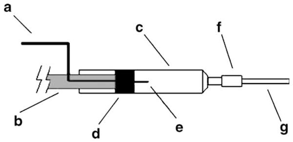
Schematic diagram of a module for separated electrophoresis (MSE). (a) voltage source cable; (b) syringe plunger; (c) 1-mL syringe barrel; (d) syringe plunger rubber; (e) platinum wire; (f) silicone tube bushing; and (g) polyethylene tube. deJesus et al. (2006) Electrophoresis Copyright Wiley-VCH Verlag GmbH & Co. KGaA. Reproduced with permission

Fonslow et al. minimized the problem of electrolysis bubbles by using channel depth to isolate the electrodes from the separation channel [28]. The electrodes were fabricated in a region four times deeper than the separation channel. Using lubrication theory and velocimetry data, the authors showed that the linear velocity of the buffer in the electrode channel was 16 times faster than that in the separation channel. The increased buffer flow over the electrodes carried bubbles out of the device without interfering with the separation. An electric field as high as 589 V cm⁻¹ could be applied before Joule heating became the limiting factor. Most of the electrical resistance was concentrated within the separation channel, resulting in approximately 91% of the applied voltage being localized in the separation channel. This chip design required additional fabrication steps and a more complex buffer-pumping scheme. The device was later redesigned to allow the separation buffer to be introduced through a single access hole [49]. A recent study using this device showed peak positions within the separation channel were stable for approximately 20 min during continuous operation at 50 V cm⁻¹ [50]. Kobayashi et al. used narrow banks fabricated 1 mm wide×20 μm thick to create isolation between the electrode and separation region [51]. While they reported applied voltages of 2 kV, the authors do not discuss the efficiency of bubble removal in their device.

Electrostatic charge induction is another method for applying bubble-free μFFE. This device uses an insulating wall to segregate the electrode from the separation channel. When a charge is applied to the electrode, the adjoining insulator wall will form a dipole with the opposite charge aligned toward the electrode (Fig. 7). This transfers charge from the electrode to the inside wall of the insulator. Continuous buffer flow through the chip prevents charged species in the buffer from neutralizing the insulator’s surface charge. Electrical current and bubble formation were not detected during an isotachophoretic focusing experiment. It was reported that a breakthrough voltage limited the maximum electric field to about 180 V cm⁻¹.

Fig. 7.

Depiction of electrostatic induction. A voltage is applied to a metal electrode in contact with an insulator. The resulting induced dipole of the insulator causes an electrostatic charge in the separation channel. Lower panel: Equivalent circuit diagram. Janasek et al. (2006) Lab Chip. Reproduced by permission of The Royal Society of Chemistry

Suppression of bubble formation through electrochemical means was demonstrated by Kohlheyer et al. [43]. The oxidation–reduction of hydroquinone and p-benzoquinone (HQ) was used to replace the electrolysis of water near the electrodes. Peak stability between experiments with and without HQ showed a 2.5-fold resolution improvement. Data suggested that the maximum applied electric field was 215 V cm⁻¹ before electrolysis bubbles begin to form. It is also noted that oxidation–reduction of HQ produces substantial pH changes within the separation channel near the electrodes. This limited the effective region of the separation channel.

The various design features and methods for suppressing bubble formation have greatly improved voltage efficiency and separation resolution in μFFE. However, these methods also have their limitations. Continuous bubble-free operation of a μFFE device for long periods of time (greater than 1 h) at high fields (greater than 200 V cm⁻¹) has yet to be reported. To utilize the full potential of μFFE, the device must operate continuously, without interference of the sample separation. The integration of μFFE with other μTAS devices has yet to be achieved, in part due to ineffective long-term bubble suppression. Electrochemical suppression of electrolysis seems promising for long-term operation of μFFE, but limited voltages and pH variations are discouraging. A combined approach using electrochemical suppression and channel depth may provide better results.

μFFE detection

Detection of analytes is paramount to the success of any analytical technique. As μFFE finds applications as an analytical system, low limits of detection are critical. Most FFE systems monitor analytes via UV detection after fractionation [6], although some examples of online detection schemes have been reported [38, 52]. Analyte detection in all microfluidic devices is limited by small sample volumes and short path-lengths. In addition, on-chip detection in μFFE requires sensing across the entire width of the separation channel. Unlike detectors in HPLC or CE, where an analyte is detected as it passes a fixed point at a given time, detection must take place over a wider area because the separation in μFFE occurs in the space, not time. On-chip detection systems for μFFE devices have been developed using either a movable scanning point-source detector [21, 22, 38], or continuously imaging a broader area using a microscope and camera [26, 28, 32, 33, 36, 39, 43, 45, 46, 48] (Fig. 8). Microscope imaging is usually preferred because it requires no moving parts and allows all sample streams to be detected simultaneously. Fluorescence, electrochemical, surface enhanced Raman scattering, Fourier transform infrared, and other detection methods have been used on various μTAS systems [19]. Thus far, most μFFE devices have used fluorescence detection because of its high sensitivity and selectivity. Fluorescence excitation has been performed using excitation light from a lamp passed through the microscope, or laser-induced fluorescence. Excitation using a lamp in an epi-fluorescence arrangement is easily performed on most microscopes, making this source common for most detection systems. To improve limits of detection, some μFFE detection systems have included laser-induced fluorescence (LIF) (Fig. 9) [21, 22, 38, 49, 50]. Although providing greater excitation power, LIF setups are more complex, as they must expand the beam to illuminate a line across the separation region or provide a method for scanning the width of the chip. In addition, the laser beam must intersect the chip at a low angle to accommodate space for the detector. A few groups have avoided fluorescence detection instrumentation by limiting their studies to visible dyes [44, 45]. To date, most μFFE studies have focused on improving separation resolution and introducing new operating modes, while detection limits and methods have been largely ignored. Recently, a study of detection limits using LIF and signal averaging in μFFE has demonstrated detection limits as low as 15 pmol L⁻¹ for fluorescein [50]. To achieve this limit of detection up to 2000 sequential μFFE images were collected and averaged in less than 5 min. The continuous nature of μFFE separations allowed so many data points to be collected in such a short time. Using traditional separation methods, signal averaging of multiple of separations is impractical, due to the time required to perform multiple separations and the reproducibility required between separations.

Fig. 8.

On-chip fluorescent detection systems for μFFE. (a) A laser line is projected across the width of the separation channel for excitation. Fluorescent signal is imaged by microscope and recorded by a CCD camera. (b) Similar setup to (a), but excitation is done by light projected though the microscope optics. (c) A laser dot on the chip excites a small portion of the separation channel. Fluorescent signal is recorded using a photomultiplier tube. A translating stage scans the chip through the detection window to acquire data across the width of the separation channel

Fig. 9.

μFFE Separation of three fluorescent dyes rhodamine 123 (1), rhodamine 110 (2), and fluorescein (3). (a) On-chip LIF imaging of dyes at the detection zone. (b) A linescan of the same μFFE separation. Turgeon and Bowser (2009) Electrophoresis Copyright Wiley-VCH Verlag GmbH & Co. KGaA. Reproduced with permission

Detection methods other than fluorescence have been suggested. In a recent review, Kohlheyer et al. proposed surface plasmon resonance (SPR) detection [53] but thus far no data have been published in the literature. Janasek et al. have suggested the use of a two-dimensional contactless conductivity detector to avoid fluorescence labeling and nonfluorescent spacers in their μFFITP devices [33]. To date, the use of conductivity detectors has not been reported.

Applications

Continuous sample separation and detection gives μFFE unique advantages over conventional separation techniques such as HPLC or CE. μFFE has been proposed for sample pre-treatment in μTAS devices [22]. The use of online detection also makes this device ideal for real time monitoring of chemical processes [22]. As with other electrophoresis methods, various modes of operation for μFFE have been developed, including zone electrophoresis (ZE), isoelectric focusing (IEF), and isotachophoresis (ITP). Most μFFE studies to date have been proof-of-concept experiments to show improvements in chip design, peak resolution, and chip fabrication but applications of this technique are beginning to emerge.

Micro free-flow zone electrophoresis (μFFZE)

A variety of different zone electrophoresis separations using μFFE devices have been described in the literature. The first μFFE chips separated fluorescently labeled amino acids by zone electrophoresis [21]. A following study using the same device showed μFFE was capable of separating large biomolecules such as bradykinin, ribonuclease A, and human serum albumin [22]. This device was limited to an electric field of 50 V cm⁻¹, with an estimated 2.5 V cm⁻¹ in the separation channel. The reported peak capacity was eight peaks cm⁻¹. Later, Kobayashi et al. separated two proteins, cytochrome C and myoglobin [51], in an all-glass chip with a large separation channel (56.5 mm wide× 35 mm long×30 mm deep). Electric fields as high as 285 V cm⁻¹ were applied to achieve continuous separation. The first PDMS μFFE chip separated the fluorescent dyes fluorescein and rhodamine 110 and labeled amino acids [34]. The device achieved separation in 72 ms with a reported electric field strength of 137 V cm⁻¹ in the separation channel. Fonslow et al. separated a mixture of the fluorescent dyes fluorescein, rhodamine 110, and rhodamine 123 to show the feasibility of their multiple-depth chip design and study the effect of separation conditions [28, 29, 32]. Their first all-glass device had a maximum electric field in the separation channel of 283 V cm⁻¹ [32]. While this device was limited by electrolysis bubbles, a later design featuring deeply etched electrode regions reached fields of 586 V cm⁻¹ in the separation channel [28]. Kohlheyer et al. also used fluorescent dyes to validate their μFFE device [27]. Fluorescein and rhodamine B were separated and stream positions within the chip were controlled by changing the flow rates at the buffer inlets.

Micro free-flow isoelectric focusing (μFFIEF)

Isoelectric focusing is another common mode of separation common in CE and FFE that has been demonstrated in μFFE. IEF separates molecules on the basis of their isoelectric point (pI). A pH gradient is established within the separation chamber as the electric field is applied. Electrolysis of water at the electrodes and ampholyte buffer mixtures are used to create the pH gradient [37, 46]. Charged analytes migrate through the pH gradient until they reach a pH zone equal to their pI (Figs. 9 and 10). Any deviation from this position causes the molecule to become charged and refocus. This focusing limits the effects of diffusional brand broadening in IEF. μFFIEF was first introduced by Xu et al. [37] using a device previously reported for μFFE [34]. Miniaturization is beneficial to IEF because it reduces the distances molecules must travel to focus. Xu showed that miniaturization scaling laws applied to μFFIEF reducing the focusing time of their devices. According to the scaling laws for molecular mass transport, with a tenfold decrease in size, separation should occur 100 times faster [20]. Compared with conventional FFIEF, samples were concentrated 400 times faster than previously reported [37].

Fig. 10.

High-resolution isoelectric focusing of seven fluorescent pH markers using a μFFE chip. A gradient from 4 to 10 pH units was established using preseparated ampholytes. The fluorescent marker had pIs of 4, 5.1, 6.2, 7.2, 8.1, 9, and 10.3. Reprinted in part with permission from Kohlheyer et al. (2007) Anal. Chem. Copyright 2007 American Chemical Society

A number of notable separations have been achieved using μFFIEF. The first μFFIEF device focused fluorescent dyes and labeled angiotensins I and II [37]. Lu et al. separated subcellular organelles at low voltages but required long focusing times of about 6 min [46]. Song et al. presented a μFFIEF device in which no external electric field was applied [54]. The device created a diffusion potential by placing the sample between two high ionic-strength buffers. Using this device they were able to separate a mixture of peptides and proteins. Kohlheyer et al. used their device for μFFIEF to separate fluorescent markers of different pI [27]. In an improved version of this device, ampholyte buffer was introduced pre-separated in order to reduce focusing time of the analytes [48]. They achieved separation resolution of analytes with pI differences of 0.4 pH units. The separation occurred within 2.5 s and an electric field of 200 V cm⁻¹. They estimated that the devices to had a peak capacity of 16 peaks cm⁻¹. Albrecht and Jensen presented a μFFIEF device with a functionalized gel within the separation channel. The functionalized gels provided pH buffering and prevented electrolysis bubbles from entering the separation channel [36]. In a subsequent paper, Albrecht and Jensen presented the first micro free-flow device in which inline back-to-back separations were performed [35]. The first μFFIEF separation occurred using a steep pH gradient to achieve a low-resolution separation. Separated analytes flowed from one of three outlets into one of three identical separation chambers operating in parallel. In the second separation, a shallow pH gradient was used to achieve high-resolution IEF separations. This device allowed for high resolution while still utilizing a fast focusing time. The separation approach used in this device could be used in other μFFE devices to more quickly achieve high-resolution separations. A number of different proteins were separated using this device.

Micro free-flow isotachophoresis (μFFITP)

Isotachophoresis is used to separate and concentrate large volumes of sample by placing the sample between electrolyte buffers with differing mobilities. It has been used extensively in capillary electrophoresis and in free-flow [6, 55] and μFFE [33]. In these experiments, the electric field within the buffer is inversely proportional to the conductivity of the buffer. The leading electrolyte is chosen to have a mobility faster than the analyte while the terminating buffer has a slower mobility. The analytes stack into zones between the leading and terminating buffers. The analytes concentrate so that the conductivity of the zones match those of the leading and trailing electrolytes. FFITP can be used to continuously concentrate a sample stream. μFFITP is presented as a method for pre-concentrating small sample volumes while utilizing the advantages of continuous flow for possible integration with other μTAS devices [33]. Mathematical modeling has been performed for optimization of FFITP [56], but to date the validity of these models with regard to μFFITP has not been confirmed experimentally.

Only a few separations using μFFITP have been reported in the literature. Janasek et al. first demonstrated μFFITP by focusing fluorescein, acetylsalicylic acid, and eosin G (Fig. 11) [33]. The applied electric field strength was 525 V cm⁻¹ with a residence time in the chamber of 50 s. With a second μFFITP device using electrostatic induction, a maximum electric field of 180 V cm⁻¹ was achieved in the separation chamber [26].

Fig. 11.

Separation of fluoresce-in and eosin G using μFFE isotachophoresis. TE and LE are abbreviations for terminating and leading electrolytes, respectively. Reprinted with permission from Janasek et al. (2006) Anal. Chem. Copyright 2006 American Chemical Society

Micro free-flow field-step electrophoresis (μFFFSE)

The final mode of separation in FFE is field-step electrophoresis. In field-step electrophoresis, high conductivity buffers are used along the edges of the separation chamber. This creates a “wall” in which the mobility of the sample will decrease, thus causing the band to focus in a manner similar to that in ITP [6]. The first use of μFFFSE was briefly reported by Kohlheyer et al. in a recent review [53]. The authors reported the separation and focusing of fluorescein from rhodamine B, but at the time of this manuscript, no further data has been published.

Dynamic μFFE separations

Although the separations described above represent progress in μFFE design, none seek to capitalize on the continuous flow advantages of μFFE. Fonslow and Bowser presented the first application of μFFE which truly relies on continuous flow [49]. They used μFFE to continuously monitor a free zone separation as the buffer conditions of the separation were varied over time. This allowed the effect of a range of separation conditions to be observed over a period of several minutes. Huh et al. used μFFE for continuous removal of urea from a protein sample [57]. The objectives of integrating μFFE with other μTAS devices or real-time monitoring of separated analytes using μFFE have yet to be realized, but these recent trends in μFFE show the devices beginning to move from proof of concept to real-world devices.

Conclusion

The strength of FFE separation devices is the ability to continuously introduce, separate, and detect a given analyte. Miniaturization of FFE has improved separation capacities by eliminating Joule heating. Miniaturization has made μFFE suitable for integration with other μTAS devices. Improvements in device design have increased the effective separation power and improved resolution. Various methods for suppressing the effects of electrolysis bubbles have also improved separation resolution. Research to date has provided enough improvements to allow research into applications for which μFFE is uniquely suited. The implementation of μFFE in bioanalytical assays and sample pre-treatment integrated with other microfluidic devices is on the near horizon.

Biography

Michael T. Bowser is currently an Associate Professor at the University of Minnesota where he has been a faculty member in the Department of Chemistry since 2000. Michael was the 2005 recipient of the ACS Award for Young Investigators in Separation Science. His research interests include microfluidic devices, high-speed neurotransmitter measurements and techniques for isolating high-affinity aptamers.

References

- 1.Dolnik V. Electrophoresis. 2008;29:143–156. doi: 10.1002/elps.200700584. [DOI] [PubMed] [Google Scholar]
- 2.Heller C. Electrophoresis. 2001;22:629–643. doi: 10.1002/1522-2683(200102)22:4<629::AID-ELPS629>3.0.CO;2-S. [DOI] [PubMed] [Google Scholar]
- 3.Kostal V, Arriaga E. Electrophoresis. 2008;29:2578–2586. doi: 10.1002/elps.200700917. [DOI] [PMC free article] [PubMed] [Google Scholar]
- 4.Barrolier VJ, Watzke E, Gibian HZ. Naturforschung. 1958;13B:754. [PubMed] [Google Scholar]
- 5.Hannig K. Z Anal Chem. 1961;181:244–254. [Google Scholar]
- 6.Roman MC, Brown PR. Anal Chem. 1994;66:86–94. [Google Scholar]
- 7.Pruski Z, Kasicka V, Mudra P, Stepanek J, Smekal O, Hlavack J. Electrophoresis. 1990;11:932–986. doi: 10.1002/elps.1150111109. [DOI] [PubMed] [Google Scholar]
- 8.Zeiller K, Loser R, Pascher G, Hannig K. Hoppe-Syler’s Z Physiol Chem. 1975;356:1225–1244. doi: 10.1515/bchm2.1975.356.2.1225. [DOI] [PubMed] [Google Scholar]
- 9.Rodkey LS. Appl Theor Electrophor. 1990;1:243–247. [PubMed] [Google Scholar]
- 10.Kessler R, Manz H-J. Electrophoresis. 1990;11:979–980. doi: 10.1002/elps.1150111119. [DOI] [PubMed] [Google Scholar]
- 11.Hoffstetter-Kuhn S, Wagner H. Electrophoresis. 1990;11:451–456. doi: 10.1002/elps.1150110603. [DOI] [PubMed] [Google Scholar]
- 12.Nath S, Schutte H, Weber G, Hustedt H, Deckwer W-D. Electrophoresis. 1990;11:937–941. doi: 10.1002/elps.1150111110. [DOI] [PubMed] [Google Scholar]
- 13.Knisley KA, Rodkey LS. Electrophoresis. 1990;11:927–931. doi: 10.1002/elps.1150111108. [DOI] [PubMed] [Google Scholar]
- 14.Clifton MJ, Jouve N, de Balmann H, Sanchez V. Electrophoresis. 1990;11:913–919. doi: 10.1002/elps.1150111106. [DOI] [PubMed] [Google Scholar]
- 15.Poggel M, Melin T. Electrophoresis. 2001;22:1008–1015. doi: 10.1002/1522-2683()22:6<1008::AID-ELPS1008>3.0.CO;2-A. [DOI] [PubMed] [Google Scholar]
- 16.Krivankova L, Bocek P. Electrophoresis. 1998;19:1064–1074. doi: 10.1002/elps.1150190704. [DOI] [PubMed] [Google Scholar]
- 17.Rhodes PH, Snyder RS. Electrophoresis. 1986;7:113. [Google Scholar]
- 18.Hannig K, Wirth H, Meyer B-H, Zeiller K. Hoppe-Seyler’s Z Physiol Chem. 1975;356:1209–1223. doi: 10.1515/bchm2.1975.356.2.1209. [DOI] [PubMed] [Google Scholar]
- 19.Dittrich PS, Tachikawa K, Manz A. Anal Chem. 2006;78:3887–3907. doi: 10.1021/ac0605602. [DOI] [PubMed] [Google Scholar]
- 20.Manz A, Eijkel JCT. Pure Appl Chem. 2001;73:1555–1561. [Google Scholar]
- 21.Raymond D, Manz A, Widmer HM. Anal Chem. 1994;66:2858–2865. [Google Scholar]
- 22.Raymond D, Manz A, Widmer HM. Anal Chem. 1996;68:2515–2522. doi: 10.1021/ac950766v. [DOI] [PubMed] [Google Scholar]
- 23.Kasicka V, Prusik Z, Pospisek J. J Chromatogr. 1992;608:13–22. [Google Scholar]
- 24.Kasicka V, Prusik Z, Sazelova P, Jiri J, Barth T. J Chromatogr A. 1998;796:211–220. doi: 10.1016/s0021-9673(97)01114-x. [DOI] [PubMed] [Google Scholar]
- 25.Giddings JC. Unified separation science. Wiley; New York: 1991. [Google Scholar]
- 26.Janasek D, Schilling M, Manz A, Franzke J. Lab Chip. 2006;6:710–713. doi: 10.1039/b602815b. [DOI] [PubMed] [Google Scholar]
- 27.Kohlheyer D, Besselink GAJ, Schlautmann S, Schasfoort RBM. Lab Chip. 2006;6:374–380. doi: 10.1039/b514731j. [DOI] [PubMed] [Google Scholar]
- 28.Fonslow BR, Barocas VH, Bowser MT. Anal Chem. 2006;78:5369–5374. doi: 10.1021/ac060290n. [DOI] [PubMed] [Google Scholar]
- 29.Fonslow BR, Bowser MT. Anal Chem. 2006;78:8236–8244. doi: 10.1021/ac0609778. [DOI] [PubMed] [Google Scholar]
- 30.Van Deemter JJ, Zuiderweg FJ, Flinkenberg A. Chem Eng Sci. 1956;5:271–289. [Google Scholar]
- 31.Shinohara E, Tajima N, Suzuki H, Funazaki J. Anal Sci Suppl. 2001;17:i441. [Google Scholar]
- 32.Fonslow BR, Bowser MT. Anal Chem. 2005;77:5706–5710. doi: 10.1021/ac050766n. [DOI] [PubMed] [Google Scholar]
- 33.Janasek D, Schilling M, Franzke J, Manz A. Anal Chem. 2006;78:3815–3819. doi: 10.1021/ac060063l. [DOI] [PubMed] [Google Scholar]
- 34.Zhang C-X, Manz A. Anal Chem. 2003;75:5759–5766. doi: 10.1021/ac0345190. [DOI] [PubMed] [Google Scholar]
- 35.Albrecht JW, El-Ali J, Jensen KF. Anal Chem. 2007;79:9364–9371. doi: 10.1021/ac071574q. [DOI] [PMC free article] [PubMed] [Google Scholar]
- 36.Albrecht JW, Jensen KF. Electrophoresis. 2006;27:4960–4969. doi: 10.1002/elps.200600436. [DOI] [PubMed] [Google Scholar]
- 37.Xu Y, Zhang C-X, Janasek D, Manz A. Lab Chip. 2003;3:224–227. doi: 10.1039/b308476k. [DOI] [PubMed] [Google Scholar]
- 38.Mazereeuw M, de Best CM, Tjaden UR, Irth H, van der Greef J. Anal Chem. 2000;72:3881–3886. doi: 10.1021/ac991202k. [DOI] [PubMed] [Google Scholar]
- 39.Macounova K, Cabrera CR, Holl MR, Yager P. Anal Chem. 2000;72:3745–3751. doi: 10.1021/ac000237d. [DOI] [PubMed] [Google Scholar]
- 40.McDonald JC, Duffy DC, Anderson JR, Chiu DT, Wu H, Schueller OJA, Whitesides GM. Electrophoresis. 2000;21:27–40. doi: 10.1002/(SICI)1522-2683(20000101)21:1<27::AID-ELPS27>3.0.CO;2-C. [DOI] [PubMed] [Google Scholar]
- 41.Sia SWG. Electrophoresis. 2003;24:3563–3576. doi: 10.1002/elps.200305584. [DOI] [PubMed] [Google Scholar]
- 42.McCreedy T. Trends Anal Chem. 2000;19:396–401. [Google Scholar]
- 43.Kohlheyer D, Eijkel JCT, Schlautmann S, van den Berg A, Schasfoort RBM. Anal Chem. 2008;80:4111–4118. doi: 10.1021/ac800275c. [DOI] [PubMed] [Google Scholar]
- 44.Stone VN, Jaldock SJ, Croasdell LA, Dillon LA, Fielden PR, Goddard NJ, Thomas CLP, Brown BJT. J Chromatogr A. 2007;1155:199–205. doi: 10.1016/j.chroma.2006.12.031. [DOI] [PubMed] [Google Scholar]
- 45.deJesus DP, Blanes L, doLago CL. Electrophoresis. 2006;27:4935–4942. doi: 10.1002/elps.200600137. [DOI] [PubMed] [Google Scholar]
- 46.Lu H, Gaudet S, Schmidt MA, Jensen KF. Anal Chem. 2004;76:5705–5712. doi: 10.1021/ac049794g. [DOI] [PubMed] [Google Scholar]
- 47.Macounova K, Cabrera CR, Yager P. Anal Chem. 2001;73:1627–1633. doi: 10.1021/ac001013y. [DOI] [PubMed] [Google Scholar]
- 48.Kohlheyer D, Eijkel JCT, Schlautmann S, van den Berg A, Schasfoort RBM. Anal Chem. 2007;79:8190–8198. doi: 10.1021/ac071419b. [DOI] [PubMed] [Google Scholar]
- 49.Fonslow BR, Bowser MT. Anal Chem. 2008;80:3182–3189. doi: 10.1021/ac702367m. [DOI] [PMC free article] [PubMed] [Google Scholar]
- 50.Turgeon RT, Bowser MT. Electrophoresis. 2009 (in press) [Google Scholar]
- 51.Kobayashi H, Shimamura K, Akaida T, Sakano K, Tajima N, Funazaki J, Suzuki H, Shinohara E. J Chromatogr A. 2003;990:169–178. doi: 10.1016/s0021-9673(02)01964-7. [DOI] [PubMed] [Google Scholar]
- 52.Hannig K, Wirth H, Schindler RK, Spiegel K. Hoppe-Seyler’s Z Physiol Chem. 1977;358:753–763. doi: 10.1515/bchm2.1977.358.2.753. [DOI] [PubMed] [Google Scholar]
- 53.Kohlheyer D, Eijkel JCT, van den Berg A, Schasfoort RBM. Electrophoresis. 2008;29:977–993. doi: 10.1002/elps.200700725. [DOI] [PubMed] [Google Scholar]
- 54.Song Y-A, Hsu S, Stevens AL, Han J. Anal Chem. 2006;78:3528–3536. doi: 10.1021/ac052156t. [DOI] [PubMed] [Google Scholar]
- 55.Hoffstetter-Kuhn S, Kuhn R, Wagner H. Electrophoresis. 1990;11:304–309. doi: 10.1002/elps.1150110406. [DOI] [PubMed] [Google Scholar]
- 56.Kasicka V, Prusik Z. J Chromatogr A. 1987;390:27–37. [Google Scholar]
- 57.Huh YS, Park TJ, Yang K, Lee EZ, Hong YK, Lee SY, Kim DH, Hong WH. Ultramicroscopy. 2008;108:1365–1370. doi: 10.1016/j.ultramic.2008.04.085. [DOI] [PubMed] [Google Scholar]