Automated Brain Tumor Segmentation Using Spatial Accuracy-Weighted Hidden Markov Random Field

Abstract

A variety of algorithms have been proposed for brain tumor segmentation from multi-channel sequences, however, most of them require isotropic or pseudo-isotropic resolution of the MR images. Although co-registration and interpolation of low-resolution sequences, such as T2-weighted images, onto the space of the high-resolution image, such as T1-weighted image, can be performed prior to the segmentation, the results are usually limited by partial volume effects due to interpolation of low resolution images. To improve the quality of tumor segmentation in clinical applications where low-resolution sequences are commonly used together with high-resolution images, we propose the algorithm based on Spatial accuracy-weighted Hidden Markov random field and Expectation maximization (SHE) approach for both automated tumor and enhanced-tumor segmentation. SHE incorporates the spatial interpolation accuracy of low-resolution images into the optimization procedure of the Hidden Markov Random Field (HMRF) to segment tumor using multi-channel MR images with different resolutions, e.g., high-resolution T1-weighted and low-resolution T2-weighted images. In experiments, we evaluated this algorithm using a set of simulated multi-channel brain MR images with known ground-truth tissue segmentation and also applied it to a dataset of MR images obtained during clinical trials of brain tumor chemotherapy. The results show that more accurate tumor segmentation results can be obtained by comparing with conventional multi-channel segmentation algorithms.

1. Introduction

Malignant glioma is one of the common types of primary brain tumor, with an annual incidence of approximately five cases per 100,000 people per year [2,3]. Over 15,000 new cases are diagnosed in the United States annually [2]. Although relatively uncommon than other major diseases, they account for a disproportionate amount of cancer-related mortality. Despite considerable ongoing research and advances made in surgical and radiosurgical techniques and chemotherapy, the overall prognosis of malignant glioma remains poor: many new chemotherapy regimens work well in a small number of patients only. This is probably related to the extreme genetic, molecular, and tissue-level heterogeneity of brain tumors. Since different genetic mutations are likely responsible for different pathophysiologies, the treatments that exist work well in only a small fraction of patients. The importance of this problem is expected to increase with the increasing number of available chemotherapeutic agents, and hence early evaluation of patients’ responses to therapy is extremely important.

Reliable and sensitive methods of assessing the effectiveness of various therapies in brain tumor patients are important for guiding treatment decisions in individual patient, for determining optimal therapy for specific patient groups, and for evaluating new therapies. Brain tumor segmentation from Magnetic Resonance Imaging (MRI) data is becoming increasingly common in clinical evaluation of tumor response to such treatments [4, 5, 6, 7, 8]. In particular, when robust and reproducible methods are used, tumor volume and shape measures have been reported to be the most significant predictor of patient outcome to treatment [6, 7, 8, 9, 10, 11]. Manual segmentation of brain-tumor images for volume measurement has been a common practice in clinics, but it is time-consuming, labor intensive, and subject to considerable variation in intra- and inter-operator performance [12]. A consistent, accurate, automated segmentation method for clinical brain tumor segmentation and measurement is much needed.

Because brain tumors vary greatly in size and shape, automated tumor segmentation remains challenging. Since some tumors are best differentiated from adjacent normal tissue on gadolinium enhanced sequences, and others on T2-weighted, FLAIR, diffusion weighted or perfusion weighted sequences [13], multi-channel segmentation methods that incorporate several different acquisition protocols/sequences and image contrasts have been widely adopted.

A great variety of tumor segmentation methods have been proposed in the literature, and they can be briefly classified into two groups: model-based methods [14, 15, 16, 17, 18, 19] and deformation-based methods [20, 21, 22]. Multi-spectral histogram analysis of T1- and T2-weighted MRI images was first adopted for tumor labeling in [19]. In this technique, the distributions of normal tissue, tumor, and edema are estimated from the T1 and T2-weighted image channels by applying an expectation-maximization (EM) scheme [14]. A variation of the method segments tissue volumes into normal and abnormal, where abnormal tissues include both tumor and edema while normal tissues consist of white and gray matters [15]. The algorithm constrains the normal tissue distribution within certain geometric and spatial boundaries and identifies the remaining tissue as the abnormal region (tumor and edema). A graph-based approach has been proposed in [16]. In this method, a Bayesian integration model is applied to minimize the cost of graph cuts that segment tumor and edema. Alternative methods involving the iterative procedure of first applying a statistical tissue classification and then performing a nonlinear registration to an anatomic atlas have been reported in [17]. Another proposed framework uses voxel intensities, neighborhood coherences, intra-structure properties, inter-structure relationships, and user inputs as the basis of tumor segmentation [18]. On the other hand, deformable methods employing morphological operations [23], region growing [20], and level set deformations [21, 22] have also been proposed for the identification of the boundaries of tumor volumes. It is worth noting that most of the deformable tumor segmentation methods are semi-automated, since the generation of initial points or surfaces is still difficult to automate.

Despite the advances in computational methods of brain tumor segmentation, a significant issue remaining is that, due to financial cost and scanning-time constraints, clinical MRI examinations typically consist of a high-resolution structural T1-weighted images combined with a couple of low-resolution images of other weighted sequences to allow accurate visual tumor diagnosis and evaluation via multi-channel images. While this is adequate for visual qualitative clinical interpretation, automated segmentation of tumor from such data is a challenge since the images acquired are of different resolutions, especially when some sequences are of low-resolutions. Direct alignment and re-sampling of these low-resolution images to match the structural T1-weighted image will cause considerable misalignment and significant partial volume effects for low-resolution images. Directly extending the segmentation produced from the high resolution data [24] to the multi-channel images will also decrease the segmentation accuracy [25].

To deal with these problems, we propose a Spatial accuracy-weighted Hidden Markov random field and Expectation maximization algorithm, called SHE for short. In this algorithm, a spatial accuracy, representing the spatial-resample accuracy of each voxel of the re-sampled low resolution images, is introduced and used in the model updating and classification. Multi-channel brain tumor image segmentation is achieved by first aligning the low-resolution images such as T2-weighted and FLAIR images onto the T1-weighted images and then applying the SHE algorithm to segment the tumor using the EM algorithm by introducing the spatial accuracy-weighted Hidden Markov Random Field (HMRF). More weights are given to the voxels with high interpolation accuracy and vise versa. In this way, the tumor segmentation results are more accurate than treating the voxels equally. We evaluated and validated this algorithm using a set of simulated multi-channel brain MR images with known ground-truth tissue segmentation and also applied it to a dataset of MR images obtained during clinical trials of brain tumor chemotherapy. The results show that more accurate tumor segmentation results can be obtained compared with the conventional multi-channel segmentation algorithm by using the spatial accuracy-weighted HMRF algorithm.

2. Methods

The Hidden Markov Random Field (HMRF) has been widely adopted in image segmentation and has been shown to be superior to other methods of single-channel human brain MR image segmentation [25]. But when HMRF is applied to multi-channel MR image segmentation, the performance has been demonstrated to be inferior [25]. The reason is that the registration accuracy and spatial re-sampling of multi-channel images (especially the re-sampling of low resolution channels) strongly affects segmentation results. In this section, we propose to improve the performance of the HMRF model by considering the spatial accuracy of each voxel in the HMRF optimization using EM algorithm.

2.1 Spatial Accuracy Vector

A typical brain tumor MRI scan, as performed at our institution, may generate one high-resolution T1-weighted image (less than 1.5mm thickness) plus several low resolution or thick section datasets with other weightings, such as T2-weighted and fluid-attenuated inversion recovery (FLAIR) images of 6 mm slice thickness. Figure 1 shows the example images of T2-weighted and FLAIR images, and such images normally have low resolutions in z-direction.

Figure 1.

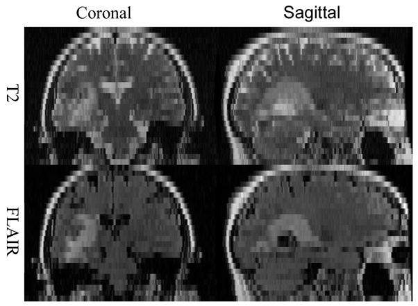
T2-weighted and FLAIR images are generally with low resolution in z-direction.

Alignment of these low-resolution images to the high-resolution T1-weighted image set, as is often done prior to multi-channel segmentation, can result in voxel misalignment and interpolation errors regardless of which of the methods is used. The process of voxel misalignment can be illustrated as follows: assuming that the task is to align an image I from one space onto another space S′, we first globally rotate and scale the image so that the transformed image I′ matches image I according to some image similarity strategy. For different modality images, mutual information is commonly used. However, as shown in Figure 2, after transformation we must interpolate image I′ according to the grids defined in S′ using linear or Spline-based methods. If the voxel is far away from its neighboring grid points, it is called a low-confidence voxel. In this situation the interpolated intensity for voxel i could be inaccurate, as represented by voxel B in Figure 2. Thus if a voxel is far away from grids it is a low-confidence voxel, and vise versa. Treating low-confidence voxels equally with high-confidence voxels could cause inaccurate model updating and poor segmentation. For example, in Figure 2, voxel A is closer to the grids of S than voxel B, it should be given higher weights when updating the class mean and variance values during segmentation than voxel B, and vise versa. For multi-channel tumor image segmentation, a similar situation applies to all the images of a given data-channel type: treating images from all channels equally could also be undesirable.

Figure 2.

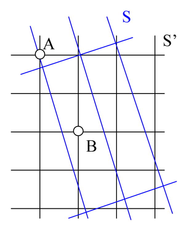
Re-sampling of a low-resolution image (S) with large slice thickness onto the space of the high-resolution image (S′). S represents the globally aligned image grids overlapping on image S′, and the traditional re-sampling methods will interpolate the intensity of S according to the grid of S′. It can be seen that the corresponding voxel A in S′ is close to the grid points of S and is of high-confidence level, however, the point of voxel B in S is far from the grid points and is of low-confidence level.

To deal with these issues, an accuracy vector for each voxel i is defined as

$${\mathbf{a}}_i={[a_{i1},\cdots ,a_{im}]}^T,$$ (1)

where m (m >1) is the number of image channels used, and the spatial accuracy level of voxel i for channel j (j=1,…, m), a_ij is defined as,

$$a_{ij}=e^{-\lambda ·\sqrt[N_i]{\prod _{k=1}^{N_i}{d}_{ij}(k)}},$$ (2)

where d_ij (k) is the Euclidean distance from voxel i to its neighboring grid point k in the low resolution image j, N_i is the number of voxels within the neighborhood of voxel i, from which the interpolated intensity value of i is obtained, and λ (λ ≥ 0) is the weighting parameter that controls the strength of spatial accuracy vector. The spatial accuracy vector can be normalized by,

$${\overline{\mathbf{a}}}_i={\mathbf{a}}_i/\sqrt[m]{\prod _{j=1}^m{a}_{ij}}.$$ (3)

2.2 Spatial Accuracy-Weighted HMRF

Zhang et al. [24] proposed the HMRF-EM method of MRI segmentation. This method has been successfully applied to tissue segmentation of multi-channel normal-brain MRI images, especially for T1- and T2-weighted images. In this paper, we report improvement of this method by using spatial accuracy weighting for multi-channel brain image segmentation in order to deal with the problems mentioned in Section 2.1. In the proposed SHE algorithm, integration of the spatial accuracy of each registered voxel improves the update of the model parameters and thus improves the final tissue classification. Suppose that y_i = [y_i1,⋯, y_im]^T is the feature vector describing each voxel i in an image in terms of the component data types, where m is the number of data channels (number of MR images), x_i ∈ L (L ∈{1, 2, ⋯, l_max}) is the class label for each voxel, and L is the class label set, according to the Maximum a Posteriori (MAP) criterion [24], the segmentation problem can be achieved by determining an estimate x̂ of the true class label x*[x₁, ⋯, x_n]^T, (n is the number of voxels), which satisfies,

$$\widehat{\mathbf{x}}=\underset{\mathbf{x}}{argmax}\{P(\mathbf{y}\mid \mathbf{x})P(\mathbf{x})\},$$ (4)

where P(x) is the prior distribution of the classification, and P(y | x) is the conditional probability of the feature vectors y of all the voxel of the images given the class label x. We assume that, for a given class label x_i = l, voxel i’s feature vector y_i follows a Gaussian distribution with parameter θ= {μ_l, Σ_l}. Thus, the Gaussian Hidden Markov Random Field (GHMRF) model [24] can be written as,

$$P({\mathbf{y}}_i\mid \mathbf{x})=P\left({\mathbf{y}}_i\mid X_{N_i},\mathbf{\theta }\right)=\sum _{l\in L}\text{g}({\mathbf{y}}_i;{\mathbf{\theta }}_l)P(l\mid X_{N_i}),$$ (5)

where X_Ni represents the class labels of the neighboring voxels of voxel i, and N_i means the neighboring voxels. P(l | X_Ni) models the conditional probability of label l given the labels of the neighboring voxels, similar to [24], and g(y_i; θ_l) is the m -dimensional Gaussian function,

$$\text{g}({\mathbf{y}}_i;{\theta }_l)=\frac{1}{\sqrt{2\pi \mid {\mathbf{\sum }}_l\mid }}{e}^{-\frac{1}{2}({\mathbf{y}}_i-{\mathbf{\mu }}_l){\mathbf{\sum }}_l^{-1}{({\mathbf{y}}_i-{\mathbf{\mu }}_l)}^T}.$$ (6)

According to [26], the prior distribution of the labels can equivalently be described by a Gibbs distribution,

$$P(\mathbf{x})=Z^{-1}exp(-U(\mathbf{x})),$$ (7)

where Z is a normalizing constant and U (X) is the energy function,

$$U(\mathbf{x})=\sum _{c\in C}{V}_c(\mathbf{x}),$$ (8)

where V_c(x) is one clique potential, and C represents all possible cliques. Here, a clique is defined as a voxel pair in which the voxels are neighbors. A homogeneous and isotropic MRF model was adopted in the GHMRF to generate the prior distribution with clique potential [27]. In our method, we use a spatial accuracy-weighted clique potential function,

$$V_c(\mathbf{x})=-\delta (x_i-x_j)\prod _{k=1}^m{a}_{ik}{a}_{jk},$$ (9)

where i and j are a pair of voxel neighbors of a clique c, and the products of accuracy levels are calculated over all the image channels m. The clique-potential is weighted by the accuracy of each data-channel’s contribution to the neighbor-pair in order to reduce the influence of a potentially-inaccurate neighborhood voxel on the current voxel. If there were no re-sampling estimation in the registration, V_c (x) becomes the original clique potential function δ(x_i − x_j).

An EM algorithm [28] is used to determine the model parameter θ for each voxel and to solve the class label x. This EM algorithm consists of two iterative steps: estimate the unobservable data needed to form a complete data set and then maximize the expected likelihood function for this complete data set. The whole SHE algorithm can be summarized as follows:

1. Initialize the segmentation/labeling x⁽⁰⁾ and the model parameter θ⁽⁰⁾.

2. M-step: maximize the expected log-likelihood using Equation (4),

   $${\mathbf{x}}^{(t)}=arg\underset{\mathbf{x}}{max}\left\{logP\left(\mathbf{y}\mid \mathbf{x},{\mathbf{\theta }}^{(t)}\right)+logP(\mathbf{x})\right\},$$ (10)

   where P(y | x, θ^(t)) and P(x) are described in Equations (5) and (7). Since solving this maximization problem directly is computationally infeasible [24], the Iterated Conditional Modes (ICM) algorithm [29] is adopted. The basic idea of the ICM algorithm is to use the “greedy”’ strategy in the iterative local maximization, i.e., given the images and the current labels of other voxels, the algorithm sequentially updates the label of each voxel by assuming that this label is dependent on the local neighborhood. Thus in this step, we iterate through all the voxels and each time update the labels of one voxel. Notice that the newly updated labels are not immediately used to calculate the labels of the subsequent voxels, and the labels are updated after all the image voxels are iterated.
3. E-step: estimate the model parameter θ^(t+1) by calculating,

   $${\mathbf{\mu }}_l^{(t+1)}={\left[\frac{{\sum }_{i\in S^{\prime }}{P}^{(t)}(l\mid {\mathbf{y}}_i)(a_{ik}{y}_{ik})}{{\sum }_{i\in S^{\prime }}{P}^{(t)}(l\mid {\mathbf{y}}_i)a_{ik}}\right]}_k,k=1,\dots ,m;l\in L$$ (11)

   and

   $${\mathbf{\sum }}_l^{(t+1)}={\left[\frac{{\sum }_{i\in S^{\prime }}{P}^{(t)}(l\mid {\mathbf{y}}_i)(a_{ik}(y_{ik}-u_{ik}))\left(a_{ij}(y_{ij}-u_{ij})\right)}{{\sum }_{i\in S^{\prime }}{P}^{(t)}(l\mid {\mathbf{y}}_i)(a_{ik}{a}_{ij})}\right]}_{kj},k,j=1,\dots ,m;l\in L,$$ (12)

   where P^(t) (l | y_i) is the posterior distribution for voxel i,

   $$P^{(t)}(l\mid {\mathbf{y}}_i)=\frac{P^{(t)}({\mathbf{y}}_i\mid l,\mathbf{\theta })P^{(t)}(l\mid X_{N_i})}{P({\mathbf{y}}_i)}.$$ (13)

   It can be seen that in this EM formulation, the parameters ${\mathbf{\mu }}_l^{(t+1)}$ and ${\mathbf{\sum }}_l^{(t+1)}$ are calculated using the accuracy weighting vector a in the M step, and more weights are given to the voxels with high-confidence, and vice versa.

4. Let t = t + 1 and repeat steps 2 and 3 until convergence, i.e. the label change in two consequent iterations is smaller than a prescribed threshold, or the maximal number of iterations has been reached.

Notice that the potential bias field has been removed before performing SHE, by applying the bias-field correction method [30] in order to deal with the intensity inhomogeneity that commonly exists in MRI images. In case that lack prior information, the widely-used discriminate-measure threshold method [31] would be used to estimate the initial segmentation. In this paper, we use a similar initial-segmentation method that maximizes the inter-class variances while minimizing the intra-class variances as used in [24].

3. SHE for Brain Tumor Segmentation

3.1 Brain Tumor Segmentation

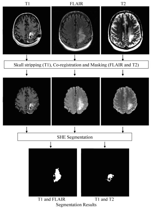
The computational framework of SHE for brain tumor segmentation is outlined in Figure 3. In this framework, the FLAIR and T2-weighted images are first co-registered onto the space of the T1-weighted high resolution images, and the accuracy weightings are calculated after the co-registration. In the co-registration, more than 80% of the voxels in the transformed images have to be interpolated from neighboring voxels that were more than 1mm away. After co-registration, skull-stripping is performed on the T1-weighted images [32].

Figure 3.

The framework of SHE segmentation of MR brain images for tumor segmentation.

By using the skull-stripped T1-weighted image as the mask, the skull is removed from the T2-weighted and FLAIR images. As shown in Figure 3, the SHE algorithm is then applied to the multiple channels for tumor segmentation. In our experiments, we used T1- and T2-weighted images to segment the non-enhanced tumor, and used T1-weighted and FLAIR images to segment the FLAIR enhanced tumor. Similar procedures introduced in Section 2.2 were applied in these two steps.

In the experiment, we evaluated the performance of SHE in segmenting brain glioma from T1-weighted, T2-weighted, and FLAIR images. Next subsection briefly summarize the datasets and evaluation methods.

3.2 Evaluation of SHE Using Simulated and Real MRI Datasets

Simulated datasets: to validate the proposed SHE algorithm, MRI images with ground-truth tissue labels were obtained from the BrainWeb [1], including T1-weighted normal brain images with 1mm slice thickness, 5% noise and 20% intensity non-uniformity. Axial, sagittal, and coronal images, with 10mm slice thickness were then extracted from the isotropic T1-weighted image set by down-sampling the data in corresponding directions. Although the low-resolution channels are simulated by down-sampling the T1-weighted images and there are no tumors in the images, the simulated data is sufficient to test the performance using spatial accuracy-weighted HMRF in image segmentation.

Real datasets

MRI data from 15 patients with brain gliomas were used in this study. The dataset consisted of high resolution T1-weighted images acquired either pre or post-contrast with 0.94mm × 0.94mm × 1.5mm voxel resolution and T2-weighted and FLAIR images of 0.47mm × 0.47mm × 6mm voxel resolution. Contrast-enhanced T1-weighting provides high signal intensity in the tumor region but poor contrast between the enhanced tumor and the gray matter. The regions of high signal intensity in the FLAIR images (corresponding to the “FLAIR volume” in [14]) include both non-enhancing and enhancing tumor. The volume of abnormal high intensity in the T2-weighted images is similar, but FLAIR images provide higher contrast between the abnormal volume and the GM.

In addition to visual evaluation, quantitative measures are also used to compare the segmentation results. There are several similarity methods for quantitatively comparing binary segmentations, including Jaccard [34], Tanimoto [35], Simple Matching [36], Volume Similarity [37], and Russel and Rao (RR) [38]. In this work, we compared the segmentation results by measuring their Jaccard Similarities and their Volume Similarities. These two similarity measurement methods can be understood by considering two binary segmentations I₁ and I₂, which have been registered to the same grid space S. Let A = {a ∈ S, I₁(a) =1} and B = {b ∈ S, I₂ (b) =1} represent the foregrounds of the two segmentations. Consequently, A̅ and B̅ are the backgrounds of I₁ and I₂. In this study, the tumor and enhanced-tumor volumes are relatively small. That is, |A̅| ≫ |A| and |B̅| ≫ |B|, where |.| represents the volume of the segmented tumors or the background (non-tumor regions). The Jaccard Similarity (JC)

$$JC=\frac{\mid A\cap B\mid }{\mid A\cup B\mid }$$ (15)

measures the overlay of two segmentations while Volume Similarity (VS)

$$VS=1-\frac{\mid \mid A\mid -\mid B\mid \mid }{\mid A\mid +\mid B\mid }$$ (16)

compares the volumes of each segmentation without considering their positions.

4. Results

4.1 Validation Results Using Simulated MR Brain Images

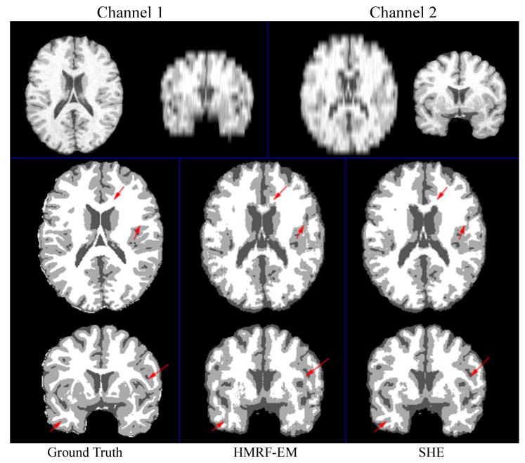
Both the original HMRF-EM method in [24] and the proposed SHE method were applied to axial and coronal images for two-channel image segmentation. Figure 4 (top row) shows such simulated low-resolution images in two channels. The first channel is the images down-sampled in z-direction, and the second channel shows the image down-sampled in y-direction. The results are shown in Figure 4 (second and third rows). Compared to the original HMRF-EM method, the SHE method generated a better segmentation. The red arrows in Figure 4 illustrate the improvement in tissue-segmentation in white matter. The sensitivity and specificity of these two segmentation methods are shown in Table 1. It can be seen that SHE increased the sensitivity of gray matter (GM) segmentation from 65.4% to 72.6% and slightly improved the sensitivities of in cerebral-spinal fluid (CSF) and white matter (WM) segmentation.

Figure 4.

Normal brain tissue segmentation results using two channels. Channel 1 and 2 are axial and coronal T1 images with 10mm slice thickness, respectively.

Table 1.

Normal brain tissue segmentation using two channels.

Tissue	HMRF-EM		SHE
	Sensitivity	Specificity	Sensitivity	Specificity
CSF	0.804	0.861	0.837	0.867
GM	0.654	0.827	0.726	0.844
WM	0.812	0.858	0.824	0.915
Average	0.757	0.849	0.796	0.875

We also segmented the three channels, i.e., down sampled images in x, y, and z directions. The result is shown in Table 2: the sensitivity of WM segmentation increased from 75.7% to 87.2% after the integration of the spatial accuracy vector. These results demonstrate that the proposed spatial accuracy weighting scheme significantly improves the results of the SHE algorithm in brain tissue segmentation. The underlying reason is that potential higher weights are given to the voxels with high interpolation confidence across all the channels and spatial relationship has been modeled effectively using the HMRF model. In this way, the SHE algorithm reduces the side effect caused by the blurry interpolated low-resolution images, and thus yields more accurate segmentation results than HMRF-EM algorithm.

Table 2.

Normal brain tissue segmentation using three channels.

Tissue	HMRF-EM		SHE
	Sensitivity	Specificity	Sensitivity	Specificity
CSF	0.843	0.858	0.867	0.878
GM	0.703	0.802	0.711	0.891
WM	0.757	0.932	0.872	0.912
Average	0.768	0.864	0.817	0.894

4.2 Brain Tumor Segmentation

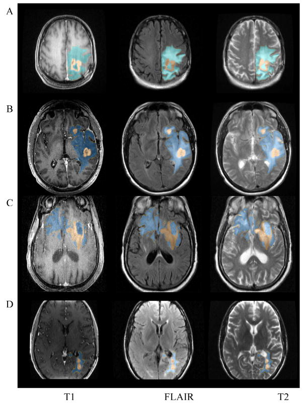
We applied the proposed algorithm on the dataset of 15 patients, and Figure 5 shows typical segmentation results from four of them (referred to as subject A, B, C, and D respectively). The segmentation results have been overlaid on the original MRI images. High resolution T1-weighted images of subjects A and C were acquired pre-Gadolinium and those of subjects B and D were acquired post-Gadolinium. Although the non-enhancing and enhancing tumor volumes vary significantly in size, shape, and position, SHE successfully segmented both the non-enhancing and enhancing-tumor volumes in both cases.

Figure 5.

An example of the brain tumor and enhancement segmentation results. Blue: edema; Brown: tumor.

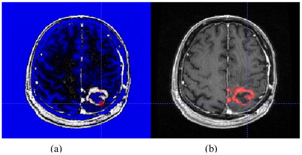
To evaluate SHE algorithm, we compared its automated segmentation results with the results of semi-automated manual segmentation performed under expert supervision. The semi-automated segmentation was performed by two experts using ITKSnap software [33]. As it is difficult for raters to distinguish abnormal FLAIR volume from CSF on the T2-weighted images, the raters segmented enhancing tumor volumes from post-Gadolinium T1-weighted images and non-enhancing tumor volumes from FLAIR images. On each image set, the raters drew several 3D spots inside the volume of abnormality and used ITKSnap to create a boundary which was then revised as needed. This is illustrated in Figure 6. Segmentation of each FLAIR and post-Gadolinium T1-weighted images took approximately 20 minutes per subject.

Figure 6.

Semi-automatic tumor segmentation using ITKSnap. (a) Preprocessing with selection of initial spots; (b) final segmentation result.

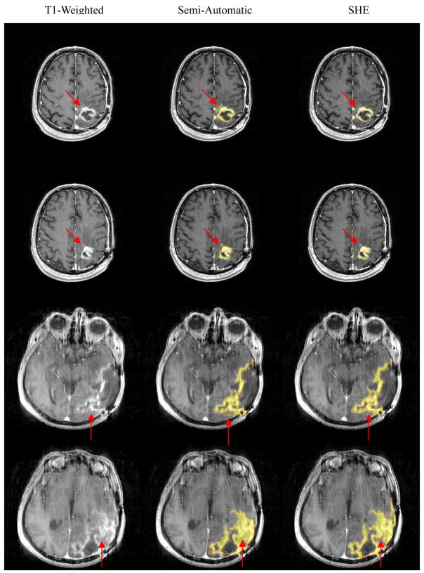
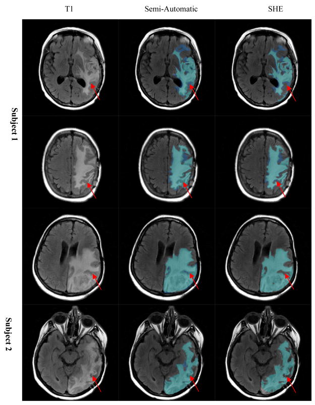
Examples of semi-automated segmentation results and SHE segmentation results are shown in Figures 7 and 8. Figure 7 shows the segmentation results using T1-weighted and T2-weighted images, and Figure 8 shows the segmentation results using contrast-enhanced T1 images and FLAIR images. The SHE segmentation results correspond more closely to the boundaries of abnormality on the source images than the semiautomated segmentation results as illustrated by the red arrows in Figures 7 and 8, possibly due to operator fatigue during manual segmentation. For example, the SHE results match the intensities of T1-weighted or contrast-enhanced T1 images better than the semi-automated results, and also there are some artificial lines/effect in the semi-automated results, which might be caused by some manual assignment of voxels to tumor regions.

Figure 7.

Brain tumor segmentation results: visual comparison between manual (semi-automatic) and automatic methods.

Figure 8.

Enhancement segmentation result: visual comparison between manual (semi-automatic) and automatic (SHE) methods.

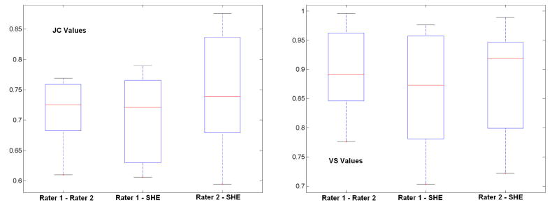
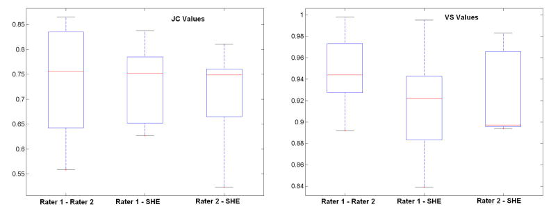
Quantitative comparisons between the semi-automated segmentation results by rater 1 and rater 2, and the automated SHE segmentations of both non-enhancing and enhancing tumor are shown in Figure 9 and 10, respectively. For semi-automated segmentation, two raters manually mark the tumor with assistant of the ITKSnap software, and automated segmentation is achieved by applying the SHE algorithm. The high volume-similarity (over 0.90) between the automated and semi-automated results for both tumor and enhanced-tumor segmentation indicates that the automated segmentation method is comparable to semi-automated segmentation. Semiautomated segmentation provides reliable and consistent segmentation results between raters, as indicated by the high volume similarity between raters. The JC value between the semi-automated and automated (SHE) results is comparable to the JC value between the two semi-automated segmentation expert operators. In summary, the automated SHE segmentation provide comparable segmentation results as the semi-automated ones by raters, and it provides a highly automated tool for tumor segmentation using multi-channel images for clinical evaluation of tumor response to treatment.

Figure 9.

Similarity of segmentation results between semi-automated results by different raters and the automated results for non-enhanced tumor. “Rater 1 – Rater 2” represents the similarity between two semi-automated results of two raters, “Rater 1 - SHE” represents the similarity between semi-automated results by rater 1 and automated results; “Rater 2 - SHE” is the similarity between semi-automated results by rater 2 and the automated results.

Figure 10.

Similarity of segmentation results between semi-automated results by raters and automated results for enhancing tumor. “Rater 1 – Rater 2” represents the similarity between two semi-automated results of two raters, “Rater 1 - SHE” represents the similarity between semi-automated results by rater 1 and automated result s; “Rater 2 - SHE” is the similarity between semi-automated results by rater 2 and the automated results.

5. Discussion and Conclusion

In this paper, we proposed to use the spatial accuracy-weighted hidden Markov random field and expectation maximization for brain image segmentation from multi-channel images. The algorithm is an important improvement over the powerful HMRF-EM segmentation algorithm in dealing with multi-channel images with different resolutions, and it is especially useful to clinical MRI datasets containing a combination of low and high resolution images. Using the simulated datasets with known ground-truth, we have demonstrated that the proposed SHE algorithm yields more accurate segmentation results than HMRF-EM. Moreover, the automated segmentation results from clinical MRI data obtained during a clinical trial demonstrate robust results comparable to those obtained by manual assisted segmentation methods.

We are integrating the SHE method into a computerized system to aid the diagnosis and follow-up of glioblastoma multiforme patients. Although this method does not completely eliminate the problem of inaccuracy resulting from registration of low-resolution image data to high-resolution data, the algorithm presented suggests a promising research direction for automated segmentation of clinical brain tumor images.

Currently, it takes similar amount of time for the SHE method to segment tumor on a P4 3.0GHz 2GB memory PC (20–25 minutes). However, since the image process pipeline is fully automated, and the human operation time is greatly reduced (less than one minute per dataset), and this frees the human operators for other activities. Furthermore, with the rapid advance of parallel computing techniques and multi-core PC systems, as well as the optimization of the software, the computation time of SHE will be reduced significantly in the near future.

Finally, certain conditions affecting the results of SHE were encountered in the current study. For example, the touching of tumor voxels with the skull would cause the failure of automated skull strip step (the FSL BET software). On the other hand, intensity inhomogeneity in MR images would sometimes reduce the accuracy of segmentation as some parameters of the skull stripping and inhomogeneity correction software need to be adjusted based on individual image. In our current implementation, the skull stripping images and the inhomogeneity corrected images are displayed automatically after the preprocessing, and the SHE algorithm is called only when the users are satisfied with the preprocessing results. In our future work, we plan to address such conditions in the SHE software to prevent from sinking into the skull areas and to handle intensity inhomogeneity in the algorithm.

References

- 1.Cocosco CA, Kollokian V, Kwan RKS, et al. BrainWeb: online interface to a 3D MRI simulated brain database. NeuroImage. 1997;5(4):S425–27. [Google Scholar]
- 2.Reardon DA, Wen PY. Therapeutic Advances in the Treatment of Glioblastoma: Rationale and Potential Role of Targeted Agents. Oncologist. 2006;11:152–164. doi: 10.1634/theoncologist.11-2-152. [DOI] [PubMed] [Google Scholar]
- 3.Brandes AA. State-of-the-art treatment of high-grade brain tumors. Semin Oncol. 2003;30:4–9. doi: 10.1053/j.seminoncol.2003.11.028. [DOI] [PubMed] [Google Scholar]
- 4.Ross DA, Sandler HM, Balter JM, et al. Imaging changes after stereotactic radiosurgery of primary and secondary malignant brain tumors. Journal of Neuro-Oncology. 2002;56(2):175–181. doi: 10.1023/a:1014571900854. [DOI] [PubMed] [Google Scholar]
- 5.Samnick S, Bader JB, Hellwig D, et al. Clinical value of iodine-123- alpha-methyl- L-tyrosine single-photon emission tomography in the differential diagnosis of recurrent brain tumor in patients pretreated for glioma at follow-up. J Clin Oncol. 2002;20:396–404. doi: 10.1200/JCO.2002.20.2.396. [DOI] [PubMed] [Google Scholar]
- 6.Schlemmer HP, Bachert P, Henze M, et al. Differentiation of radiation necrosis from tumor progression using proton magnetic resonance spectroscopy. Neuroradiology. 2002;44:216–222. doi: 10.1007/s002340100703. [DOI] [PubMed] [Google Scholar]
- 7.Kumar AJ, Leeds NE, Fuller GN, et al. Malignant gliomas: MR imaging spectrum of radiation therapy– and chemotherapy-induced necrosis of the brain after treatment. Radiology. 2000;217:377–384. doi: 10.1148/radiology.217.2.r00nv36377. [DOI] [PubMed] [Google Scholar]
- 8.Vaidynathan M, Clarke LP, Hall LO, et al. Monitoring brain tumor response to therapy using MRI segmentation. Magn Reson Imaging. 1997;15:323–334. doi: 10.1016/s0730-725x(96)00386-4. [DOI] [PubMed] [Google Scholar]
- 9.Pan DH, Guo WY, Chung WY, et al. Early effects of Gamma Knife surgery on malignant and benign intracranial tumors. Stereotact Funct Neurosurg. 1995;64:19–31. doi: 10.1159/000098761. [DOI] [PubMed] [Google Scholar]
- 10.Black PM, Moriarty T, Alexander E, et al. Development and implementation of intraoperative magnetic resonance imaging and its neurosurgical applications. Neurosurgery. 1997;41:831–845. doi: 10.1097/00006123-199710000-00013. [DOI] [PubMed] [Google Scholar]
- 11.Jannin P, Morandi X. Surgical models for computer assisted neurosurgery. Neuroimage. 2007;37:783–791. doi: 10.1016/j.neuroimage.2007.05.034. [DOI] [PubMed] [Google Scholar]
- 12.Joe BN, Fukui MB, Meltzer CC, et al. Brain tumor volume measurement: comparison of manual and semiautomated methods. Radiology. 1999;212:811–816. doi: 10.1148/radiology.212.3.r99se22811. [DOI] [PubMed] [Google Scholar]
- 13.Just M, Higer HP, Schwarz M, et al. Tissue characterization of benign tumors: use of NMR-tissue parameters. Magn Reson Imaging. 1988;6:463–472. doi: 10.1016/0730-725x(88)90482-1. [DOI] [PubMed] [Google Scholar]
- 14.Prastawa M, Bullitt E, Moon N, et al. Automatic brain tumor segmentation by subject specific modification of atlas priors. Academic Radiology. 2003;10:1341–1348. doi: 10.1016/s1076-6332(03)00506-3. [DOI] [PMC free article] [PubMed] [Google Scholar]
- 15.Prastawa M, Bullitt E, Ho S, et al. Robust estimation for brain tumor segmentation. MICCAI. 2003:530–537. [Google Scholar]
- 16.Corso JJ, Sharon E, Yuille A. Multilevel segmentation and integrated Bayesian model classification with an application to brain tumor segmentation. MICCAI. 2006:790–798. doi: 10.1007/11866763_97. [DOI] [PubMed] [Google Scholar]
- 17.Kaus MR, Warfield SK, Nabavi Arya, et al. Automated segmentation of MR images of brain tumors. Radiology. 2001;218(2):586–591. doi: 10.1148/radiology.218.2.r01fe44586. [DOI] [PubMed] [Google Scholar]
- 18.Gering DT, Grimson WEL, Kikinis R. Recognizing deviations from normalcy for brain tumor segmentation. MICCAI. 2002:388–395. [Google Scholar]
- 19.Clark MC, Hall LO, Goldgof DB, et al. Automatic tumor segmentation using knowledge-based techniques. IEEE Transactions on Medical Imaging. 1998;17:238–251. doi: 10.1109/42.700731. [DOI] [PubMed] [Google Scholar]
- 20.Moonis G, Liu J, Udupa JK, et al. Estimation of tumor volume with fuzzy-connectedness segmentation of MR images. Am J Neuroradiol. 2002;23:356–363. [PMC free article] [PubMed] [Google Scholar]
- 21.Ho S, Bullitt E, Gerig G. Level set evolution with region competition: automatic 3-D segmentation of brain tumors. In Proc. 16 Int Conf on Pattern Recogntion ICPR; 2002. pp. 532–535. [Google Scholar]
- 22.Xie K, Yang J, Zhang ZG, Zhu YM. Semi-automated brain tumor and edema segmentation using MRI. European Journal of Radiology. 2005;56:12–19. doi: 10.1016/j.ejrad.2005.03.028. [DOI] [PubMed] [Google Scholar]
- 23.Zhu Y, Yan H. Computerized tumor boundary detection using a hopfield neural network. IEEE Transactions on Medical Imaging. 1997;16:55–67. doi: 10.1109/42.552055. [DOI] [PubMed] [Google Scholar]
- 24.Zhang Y, Brady M, Smith S. Segmentation of brain MR images through a hidden Markov random field model and the expectation-maximization algorithm. IEEE Trans Medical Imaging. 2001;20:45–57. doi: 10.1109/42.906424. [DOI] [PubMed] [Google Scholar]
- 25.Bouix S, Martin-Fernandez M, Ungar L, et al. On evaluating brain tissue classifiers without a ground truth. NeuroImage. 2007;36:1207–1224. doi: 10.1016/j.neuroimage.2007.04.031. [DOI] [PMC free article] [PubMed] [Google Scholar]
- 26.Besag J. Spatial interaction and statistical analysis of lattice systems. J Roy Stat Soc. 1974;36:192–326. ser. B. [Google Scholar]
- 27.Geman S, Geman D. Stochastic relaxation, Gibbs distributions, and the Bayesian restoration of images. IEEE Trans Pattern Anal Machine Intell. 1984;6:721–741. doi: 10.1109/tpami.1984.4767596. [DOI] [PubMed] [Google Scholar]
- 28.Dempster AP, Laird NM, Bubin DB. Maximum likelihood from incomplete data via EM algorithm. J Roy Stat Soc. 1977;39:1–38. ser. B. [Google Scholar]
- 29.Besag J. On the statistical analysis of dirty pictures. J of Royal Statist Soc. 1986;48:259–302. ser. B. [Google Scholar]
- 30.Wells WM, Grimson EL, Kikinis R, et al. Adaptive segmentation of MRI data. IEEE Trans Med Imag. 1996;15:429–442. doi: 10.1109/42.511747. [DOI] [PubMed] [Google Scholar]
- 31.Otsu N. A threshold selection method from gray-level histogram. IEEE Trans Syst Man Cybern. 1979;9:62–66. [Google Scholar]
- 32.Smith SM. Fast robust automated brain extraction. Human Brain Mapping. 2002;17(3):143–155. doi: 10.1002/hbm.10062. [DOI] [PMC free article] [PubMed] [Google Scholar]
- 33.Yushkevich PA, Piven J, Cody H, et al. User-guided level set segmentation of anatomical structures with ITK-SNAP. Insight Jounral, Special Issue on ISC/NA-MIC/MICCAI Workshop on Open-Source Software; 2005. [Google Scholar]
- 34.Jaccard P. Étude comparative de la distribuition florale dans une portion desalpes et de jura. Bulletin de la Societé Voudoise des Sciences Naturelles. 1901;37:547–579. [Google Scholar]
- 35.Rogers JS, Tanimoto TT. A computer program for classifying plants. Science. 1960;132:1115–1118. doi: 10.1126/science.132.3434.1115. [DOI] [PubMed] [Google Scholar]
- 36.Sokal RR, Michener CD. A statistical method for evaluating systematic relationships. Univ Kans Sci Bull. 1958;38:1409–1438. [Google Scholar]
- 37.Fernandez MM, Bouix S, Ungar L, et al. Two methods for validating brain tissue classififiers. MICCAI. 2005;LNCS 3749:515–522. doi: 10.1007/11566465_64. [DOI] [PMC free article] [PubMed] [Google Scholar]
- 38.Russel PF, Rao TR. On habitat and association of species of anophelinae larvae in south-eastern Madras. J Malaria Inst India. 1940;3:153–178. [Google Scholar]