Toward Realistic and Practical Ideal Observer (IO) Estimation for the Optimization of Medical Imaging Systems

Abstract

The ideal observer (IO) employs complete knowledge of the available data statistics and sets an upper limit on observer performance on a binary classification task. However, the IO test statistic cannot be calculated analytically, except for cases where object statistics are extremely simple. Kupinski et al. have developed a Markov chain Monte Carlo (MCMC) based technique to compute the IO test statistic for, in principle, arbitrarily complex objects and imaging systems. In this work, we applied MCMC to estimate the IO test statistic in the context of myocardial perfusion SPECT (MPS). We modeled the imaging system using an analytic SPECT projector with attenuation, distant-dependent detector-response modeling and Poisson noise statistics. The object is a family of parameterized torso phantoms with variable geometric and organ uptake parameters. To accelerate the imaging simulation process and thus enable the MCMC IO estimation, we used discretized anatomic parameters and continuous uptake parameters in defining the objects. The imaging process simulation was modeled by precomputing projections for each organ for a finite number of discretely-parameterized anatomic parameters and taking linear combinations of the organ projections based on continuous sampling of the organ uptake parameters. The proposed method greatly reduces the computational burden and allows MCMC IO estimation for a realistic MPS imaging simulation. We validated the proposed IO estimation technique by estimating IO test statistics for a large number of input objects. The properties of the first- and second-order statistics of the IO test statistics estimated using the MCMC IO estimation technique agreed well with theoretical predictions. Further, as expected, the IO had better performance, as measured by the receiver operating characteristic (ROC) curve, than the Hotelling observer. This method is developed for SPECT imaging. However, it can be adapted to any linear imaging system.

The ideal observer (IO) employs complete knowledge of the object statistics and sets an upper limit on observer performance for a binary classification task. Thus, the IO provides a powerful theoretical tool for assessing imaging system performance using raw data. Its performance provides a measure that is independent of subsequent processing, display, or interpretation steps in the sense that these steps cannot provide higher performance. In other words, IO performance reflects the amount of information presented in the measured data. The independence of IO performance on subsequent steps is often desirable in system design and optimization because including these steps in the optimization vastly increases the number of parameters that would have to be optimized.

However, analytic computation of IO performance is limited to cases where object statistics are extremely simple (e.g., a uniform background), and where the imaging system is simple and well characterized (e.g., spatially invariant Gaussian blurring with Gaussian or Poisson noise). Kupinski et al. have developed a Markov chain Monte Carlo (MCMC) based technique to compute the IO test statistic [1]. With known parameterization and the ability to compute the background-known-exactly (BKE) likelihood ratio, the MCMC technique allows modeling of, in principle, arbitrarily complicated object statistics and imaging systems at the expenses of significantly longer computational time. In practice, due to the extremely long computation time, application of this method has been limited to relatively simple object models, such as statistically-defined lumpy background [2], and relatively simple imaging system models, i.e., spatially invariant Gaussian blurring with Gaussian or Poisson noise [1]. Gross et al. used MCMC for IO calculations with a pinhole single photon emission computed tomography (SPECT) system model and lumpy backgrounds [3], [4]. In this study, a system with non-Gaussian blur and spatially varying blur was modeled. However, the method has not been applied to cases that include spatially varying effects in the object.

In the work presented here, we applied MCMC to estimate the IO test statistic in the context of myocardial perfusion SPECT (MPS) using a realistic analytic projector, modeling of Poisson noise statistics, and a parameterized torso phantom. To speed up the MCMC IO estimation, we have developed a method that uses a precomputed set of organ projections for a finite number of anatomic parameters. The object sampling for the MCMC estimation was discrete for the anatomic parameters and continuous for organ uptake parameters. We validated the proposed technique by investigating the properties of the resulting IO test statistics and comparing IO performance with that of a Hotelling observer.

The purpose of this work is to demonstrate and validate the MCMC IO technique as applied to MPS. While we used an analytic projector and a relatively simple phantom in this work, the technique could be easily extended to a more realistic system model (e.g., Monte Carlo simulation) and phantom. This method is developed for SPECT imaging. However, it can be adapted to any linear imaging system.

I. METHODS

A. Kupinski’s MCMC IO Estimation Method [1]

The IO uses likelihood ratio (LR), Λ(g⃑), as the decision variable

$$\mathrm{\Lambda }(\stackrel{\rightharpoonup }{g})=\frac{\text{pr}(\stackrel{\rightharpoonup }{g}|H_1)}{\text{pr}(\stackrel{\rightharpoonup }{g}|H_0)}$$ (1)

where g⃑ is the image vector and H_i is the ith hypothesis. Kupinski formulated Λ(g⃑) as an integral of the background-known-exactly (BKE) LR over the background, $\stackrel{\rightharpoonup }{b}=b(\stackrel{\rightharpoonup }{\theta })$, parameterized by θ⃑, given the image data g⃑ under hypothesis H₀ [1]. In this formulation

$$\mathrm{\Lambda }(\stackrel{\rightharpoonup }{g})={\displaystyle \int {\mathrm{\Lambda }}_{\text{BKE}}(\stackrel{\rightharpoonup }{g}|\stackrel{\rightharpoonup }{b})\text{pr}(\stackrel{\rightharpoonup }{b}|\stackrel{\rightharpoonup }{g},H_0)d\stackrel{\rightharpoonup }{b}.}$$ (2)

Kupinski has shown that, if the function b(θ⃑) is one-to-one, (2) can be expressed as an integral over θ⃑ instead of b⃑, i.e.,

$$\mathrm{\Lambda }(\stackrel{\rightharpoonup }{g})={\displaystyle \int {\mathrm{\Lambda }}_{\text{BKE}}(\stackrel{\rightharpoonup }{g}|b(\stackrel{\rightharpoonup }{\theta }))}\text{pr}(\stackrel{\rightharpoonup }{\theta }|\stackrel{\rightharpoonup }{g},H_0)d\stackrel{\rightharpoonup }{\theta }.$$ (3)

The integral in (3) can then be estimated by Monte Carlo integration, i.e.,

$$\widehat{\mathrm{\Lambda }}(\stackrel{\rightharpoonup }{g})=\frac{1}{J}{\displaystyle \sum _{j=1}^J{\mathrm{\Lambda }}_{\text{BKE}}^{(j)}}$$ (4)

where

$${\mathrm{\Lambda }}_{\text{BKE}}^{(j)}={\mathrm{\Lambda }}_{\text{BKE}}\left(\stackrel{\rightharpoonup }{g}|b\left({\stackrel{\rightharpoonup }{\theta }}^{(j)}\right)\right).$$ (5)

In (4) and (5), each θ⃑^(j) is a sample from the distribution $\text{pr}(\stackrel{\rightharpoonup }{\theta }|\stackrel{\rightharpoonup }{g},H_0)$. Therefore, the key to estimating Λ(g⃑) is generating a series of θ⃑^(j) from $\text{pr}(\stackrel{\rightharpoonup }{\theta }|\stackrel{\rightharpoonup }{g},H_0)$, then computing and averaging Λ_BKE using (4). Kupinski then proposed a Markov chain method with $\text{pr}(\stackrel{\rightharpoonup }{\theta }|\stackrel{\rightharpoonup }{g},H_0)$ as the stationary density. In this method, the resulting Markov chain is the desired series of sets of object parameters θ⃑^(j).

To obtain this Markov chain, an iterative approach is used beginning with an initial estimate θ⃑⁽⁰⁾ and a proposal function, $q(\widetilde{\stackrel{\rightharpoonup }{\theta }}|{\stackrel{\rightharpoonup }{\theta }}^{(j)})$. For each θ⃑^(j), a $\widetilde{\stackrel{\rightharpoonup }{\theta }}$ is proposed by sampling the proposal function, and is accepted by the Markov chain with a probability [5]

$$\alpha \left(\widetilde{\stackrel{\rightharpoonup }{\theta ,}}{\stackrel{\rightharpoonup }{\theta }}^{(j)}\right)=\text{min}\left[1,\frac{\text{pr}(\stackrel{\rightharpoonup }{g}|\widetilde{\stackrel{\rightharpoonup }{\theta }},H_0)\text{pr}(\widetilde{\stackrel{\rightharpoonup }{\theta })}q\left(\widetilde{\stackrel{\rightharpoonup }{\theta }|}{\stackrel{\rightharpoonup }{\theta }}^{(j)}\right)}{\text{pr}(\stackrel{\rightharpoonup }{g}|{\stackrel{\rightharpoonup }{\theta }}^{(j)},H_0)\text{pr}({\stackrel{\rightharpoonup }{\theta }}^{(j)})q\left({\stackrel{\rightharpoonup }{\theta }}^{(j)}|\widetilde{\stackrel{\rightharpoonup }{\theta }}\right)}\right].$$ (6)

Equation (6) is also known as Metropolis–Hastings algorithm [2]. In this paper, as well as in [1], a more specialized Metropolis algorithm, which considers only symmetric proposal densities is used . In this case, the proposal density in (6) cancels out, i.e., $q(\widetilde{\stackrel{\rightharpoonup }{\theta }}|{\stackrel{\rightharpoonup }{\theta }}^{(j)})/q({\stackrel{\rightharpoonup }{\theta }}^{(j)}|\widetilde{\stackrel{\rightharpoonup }{\theta }})=1$. Note that, in principle, this method can be applied to any object that can be parameterized by a statistically defined set of parameters for which the BKE likelihood ratio can be computed. In [1], this method was applied to a lumpy background object model for the case where full knowledge of the imaging system characteristics and noise properties were known.

B. Difficulties of Implementing MCMC IO Estimation in Cardiac SPECT Imaging for a Parameterized Phantom

In principle, the MCMC IO estimation can be adapted to any parameterized phantom and simulated imaging system, as shown in Fig. 1. Since we are interested in cardiac SPECT imaging, the procedure shown in Fig. 1 can be described as follows.

• Step 1)

  Propose an initial estimate of the phantom parameters, which is considered the current parameter, and generate the phantom and simulate the imaging process to obtain a background image (or signal-free projection image) b(θ⃑⁽⁰⁾) based on the current parameters. The simulation can be done using either analytical or Monte Carlo simulation.

• Step 2)

  Output the current parameter θ⃑^(j) into the Markov chain.

• Step 3)

  Propose a new set of parameters $\widetilde{\stackrel{\rightharpoonup }{\theta }}$ using the proposal function, $q(\widetilde{\stackrel{\rightharpoonup }{\theta }}|{\stackrel{\rightharpoonup }{\theta }}^{(j)})$, and simulate the corresponding phantom and background image (or signal-free projection image) $b(\widetilde{\stackrel{\rightharpoonup }{\theta )}}$.

• Step 4)

  Using Metropolis-Hastings algorithm in (6) to determine the acceptance of the new set of parameters, $\widetilde{\stackrel{\rightharpoonup }{\theta }}$. In case of acceptance, update the current parameters and the current background. In case of rejection, the current parameters and current background remain unchanged.

• Step 5)

  Repeat Steps 2–4 a large number of times to obtain a series of θ⃑⁽⁰⁾,θ⃑⁽¹⁾,θ⃑⁽²⁾ … θ⃑^(j) …

In practice, the procedure in Fig. 1 is so computationally demanding that it is practically impossible to apply. To be specific, MCMC IO estimation is an iterative approach, which requires hundreds of thousands of iterations to obtain one $\widehat{\mathrm{\Lambda }}(\stackrel{\rightharpoonup }{g)}$. For example, Kupinski used 150 000 iterations in [1]. In each iteration, in order to calculate the background b(θ⃑) the simulation of the imaging process given the phantom, parameterized by object parameters θ⃑, must be performed in Step 3. This may take seconds, using an analytical SPECT projector, or hours using a Monte Carlo SPECT projection model. Furthermore, obtaining a receiver operating characteristic (ROC) curve requires at least 50 pairs of $\widehat{\mathrm{\Lambda }}(\stackrel{\rightharpoonup }{g)}$ values. This makes MCMC IO estimation computationally impossible in such situations.

Fig. 1.

Applying the MCMC IO estimation technique in the case where a parameterized phantom and simulated system are used.

C. MCMC IO Estimation Using a Parameterized Phantom and a Precalculated Dataset for Cardiac SPECT Imaging

To make IO estimation possible for cardiac SPECT imaging, acceleration of Step 3 is required. To accomplish this, we used a parameterized torso phantom and a precalculated database of organ projections for each phantom. In what follows, we will describe the four key elements of the proposed method.

Phantom (or Object)

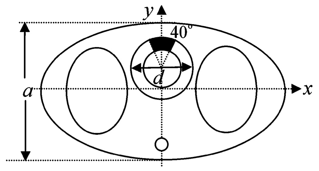
For the purpose of demonstrating the feasibility of applying MCMC IO estimation to cardiac SPECT imaging, we used a parameterized 3-D torso phantom whose central slice is shown in Fig. 2. In the phantom, we modeled heart, which is the target organ in cardiac SPECT imaging. We also modeled the body and lung, which provide the attenuation environment for the heart. A spinal cord was added at the posterior position of the torso. The kidney was omitted for simplicity. An anterior perfusion defect was also modeled that spans 40° of the myocardial wall and has a defect contrast of 1.0.

Fig. 2.

Parameterized torso phantom.

To describe the phantom, we specified two anatomic parameters, the heart size d and the body thickness a. All other anatomic parameters are determined by d and a. For example, the long axis of the lung, defined by the number of pixels, in the y direction is defined as

$$a_{\text{lung}}=a+0.75d-5$$

and the short axis of the lung in the x direction is defined as

$$b_{\text{lung}}=a\ast \text{sqrt}\left(1-\frac{{(a-0.75d)}^2}{4a^2}\right)-5.$$

Additional constraints were added to ensure that the organs are within the boundary of the body. Note that the method could be extended to a more realistic phantom described by a larger number of discrete parameters. In addition to the geometric parameters, there are three tracer uptake parameters representing the activity concentration in the body (A_body), lung (A_lung), and heart (A_heart). A 40° circumferential defect was modeled in the anterior wall. Thus, the phantom is parameterized by θ⃑₀, expressed as

$$\stackrel{\rightharpoonup }{{\theta }_0}=[da{A}_{\text{body}}{A}_{\text{lung}}{A}_{\text{heart}}].$$ (7)

Note that, since the five parameters are independent of each other, for any θ⃑₀, there exists a unique phantom.

A Precalculated Database

We first obtained N heart sizes within a certain range with equal spacing over the range, e.g., N = 50 heart sizes over the range 3–6 cm was used in the subsequent experiments. Using a similar approach, we obtained M body sizes (e.g., in this study M = 50 and body sizes range from 22 to 26 cm). The ranges for heart and body sizes are determined by that of the patient data. Since the anatomy was completely determined by d and a, this produced N × M different anatomies in the precalculated database. We used n and m to index the heart size and body thickness in the anatomical database. Thus, the parameters to describe the object become

$$\stackrel{\rightharpoonup }{\theta }=[nm{A}_{\text{body}}{A}_{\text{lung}}{A}_{\text{heart}}].$$ (8)

Compared with the parameter definition in (7), the definition in (8) replaces some of the continuous parameters with a finite number of discrete ones. Note that in the database, the heart sizes are equally spaced. In real patient data, however, the heart sizes are roughly Gaussian distributed truncated to a certain range. It should be pointed out that the distribution of the parameters in the database does not necessarily to be identical to that in the testing dataset.

In this application, the measured data are in the projection domain, and thus the database is generated in the projection domain. For each anatomy, indexed with m and n, we first separately generate projections of the heart, body, defect and lung filled with unit activity, using the attenuation map that is uniquely defined by n and m. This library of projection data is then stored. Note that in the database, all images are noise free.

MCMC IO Estimation

As discussed previously, the major difficulty in implementing MCMC IO estimation is the computational burden in simulating the projection data from a phantom parameterized by θ⃑. Using the precalculated database, this simulation process can be dramatically accelerated. For a given parameter θ⃑, we locate the corresponding anatomy using the indexes n and m, and the background image can be generated by scaling and summing the three organ projections together according to the values of A_body, A_lung, and A_heart. As a result, we can write the projection for the whole phantom as a linear combination of the projections of the lungs, body, and organs as

$$\text{prj}(\stackrel{\rightharpoonup }{\theta )}=A_{\text{body}}{\text{prj}}^{\text{body}}+A_{\text{lung}}{\text{prj}}^{\text{lung}}+A_{\text{heart}}{\text{prj}}^{\text{heart}}$$ (9)

where prj(θ⃑) is the projection data for the entire object given the parameter vector θ⃑, prj^body, prj^lung, and prj^heart are the projections with unit activities for the body, lungs, and heart, respectively. These projections are retrieved from the particular anatomy indexed with m and n. By doing so, more than 50 000 backgrounds can be generated in less than 1 s using phantoms of dimension 64 × 64 × 20.

Proposal Function

The proposal function, $q(\widetilde{\stackrel{\rightharpoonup }{\theta }}|{\stackrel{\rightharpoonup }{\theta }}^{(i)})$ in (10), was designed as a symmetric variable-at-a-time function (i.e., in each iteration, the proposal function randomly choses one parameter to propose)

$$\begin{array}{cc}q\left(\widetilde{\stackrel{\rightharpoonup }{\theta }}|{\stackrel{\rightharpoonup }{\theta }}^{(j)}\right)=\hfill & {\displaystyle \sum _i\{\frac{1}{5}{G}_i\left(A_i^{(j)}-{\tilde{A}}_i\right){\displaystyle \prod _{k\ne i}\delta \left(A_k^{(j)}-{\tilde{A}}_k\right)}}\hfill \\ \hfill & \hfill \times \delta \left(\tilde{n}-n^{(j)}\right)\delta \left(\tilde{m}-m^{(j)}\right)\}\hfill \\ \hfill & +\frac{1}{5}{P}_{\text{heart}}\left(\tilde{n}-n^{(j)}\right)\hfill \\ \hfill & \times {\displaystyle \prod _i\delta \left(A_i^{(j)}-{\tilde{A}}_i\right)\delta \left(\tilde{m}-m^{(j)}\right)}\hfill \\ \hfill & +\frac{1}{5}{P}_{\text{body}}\left(\tilde{m}-m^{(j)}\right)\hfill \\ \hfill & \times {\displaystyle \prod _i\delta \left(A_i^{(j)}-{\tilde{A}}_i\right)\delta \left(\tilde{n}-n^{(j)}\right)}\hfill \end{array}$$ (10)

where i can be heart, body, or lung, $A_i^{(j)}$ is the current activity concentration parameter for the ith organ, Ã_i is the proposed activity concentration parameter in the ith organ, and the function G_i() represents the probability density for proposing new activity concentrations for the three organs, which are assumed to follow Gaussian distributions. The discrete probability distributions P_heart and P_body were used to propose new anatomic parameters, where n and m are the current anatomy indexes and ñ and m̃ represent the proposed anatomy indexes. The discrete distribution is defined by discretizing a Gaussian distribution and sampling it at the discrete values of m. An example of the definition of P_body(m̃ − m) is shown in Fig. 3 for a Gaussian distribution with a standard deviation 1.0. P_heart(n − ñ) has a similar definition. If the proposed parameter exceeds the ranges that define the database, e.g., m is greater than M or less than 1, the proposal function has a value 0, and the proposed parameter is rejected according to the Metropolis–Hastings algorithm shown in (5).

Fig. 3.

An example of the definition of P_body (m̃−m).

D. Experiment Design

The purpose of this study was to implement and validate MCMC IO estimation for a realistic imaging system model and a parameterized phantom. We thus used the phantom shown in Fig. 2 and an analytical SPECT projector for simplicity. The proposed method, however, could be extended to more realistic phantom designs and more realistic (e.g., Monte Carlo simulated) SPECT projectors.

We began with the design of the phantom database. The two anatomic parameters to be used are equally spaced within the maximum and minimum shown in Table I. We generated a 50× 50 database, where the 50 heart sizes range from 3.0 to 6.0 cm in 0.06 cm increment, and the 50 body thickness values range from 22.0 to 26.0 cm in 0.08 cm increment. The parameters are shown in Table I. The definition of the parameters and the generation of the phantoms as described previously prevent the heart from sticking out of the body. Three activity distributions were used, assuming Gaussian distributions truncated to the maximum and minimum values, as shown in Table II. Note that one attenuation map was generated for each of the 50× 50 anatomies. The phantoms were all stored in voxelized 3-D images, 64 × 64 × 20 in dimension.

TABLE I.

Anatomic Parameters

	Maximum	Minimum
Heart diameter (cm)	6.0	3.0
Body thickness (cm)	26.0	22.0

TABLE II.

Activity Parameters

	Mean	Standard deviation	Max	Min
Heart Activity (pixel value)	140	20	180	100
Body Activity (pixel value)	30	12	54	6
Lung Activity (pixel value)	30	20	40	20

For each anatomy in the 50 × 50 database, we generated noise-free raw projection data of the heart, body, and lungs separately assuming unit activity in each organ. The projection data contained only the anterior view, for simplicity, and were 64× 20 in size. A realistic analytical SPECT projector with attenuation and distant-dependent detector response effects was used. We modeled an LEHR collimator, an emission energy of 140 keV, and a pixel size of 0.6 cm in the simulation.

To generate a projection image for the observer study, we first sampled the discrete anatomic parameters and the continuous activity parameters. The anatomical parameters were randomly sampled assuming uniform distributions, while the activity distributions were assumed to be normally distributed with parameters specified in Table II. We formed the raw projection data by selecting the appropriate projection dataset from the database and scaling the organ projections as described above. The data were then scaled to a realistic count-level and Poisson noise was simulated. To perform an IO study, we generated a total of 2000 pairs of these noisy defect-present and -absent projection images.

For each of the 2000 pairs of projection images g⃑ the MCMC IO algorithm was applied to obtain one estimated LR, $\widehat{\mathrm{\Lambda }}(\stackrel{\rightharpoonup }{g)}$. Instead of using the whole image to compute the LR, we used a region-of-interest (ROI) of the image that contains the defect (or on the corresponding position of defect-absent image). The ROI used was a horizontal profile through the projection image 44 pixels long that crossed the center of the defect.

The purpose of this study was to demonstrate the feasibility of the proposed MCMC approach using a parameterized phantom and a realistic image formation model. In order to study the convergence properties of the Markov chain, we generated chains with a large number of iterations. In order to make this computationally tractable, it was desirable to perform all the computations in memory. We thus chose to use an object described by a small number of parameters, narrow ranges of parameter values, and a relatively small number of discretized anatomies in the database. Second, in the following we validate the MCMC approach by testing the statistical properties of the LR. Due to the nonsymmetric nature of the LR, a large number of defect-present/absent pairs are needed to compute the mean and variance of the LR distributions (as described in Section II). Using the relatively simple phantom parameterization reduced the computational requirements and enabled this line of validation. Third, we would like to compare Hotelling observer and IO performance. When a large image matrix is involved, it is almost impossible to compute the Hotelling test statistic using ensemble methods, due to the difficulty of estimating and inverting the required large covariance matrix. As a result, we computed the LR for a linear 44 pixel region perpendicular to the rotation axis instead of the entire image. However, we modeled the image formation into the entire projection image and thus included contributions from voxels in the image that did not project geometrically to this region.

II. EXPERIMENTS AND RESULTS

As described previously, we generated an ensemble of 2000 pairs of defect-present and -absent projection images. In the following, we describe and present the results from two kinds of experiments performed using these data. In Section II-A, we demonstrated the convergence properties of the MCMC method by computing the Markov chain for one particular defect-present projection image; in Sections II-B–II-D, we investigated the statistical properties of the LRs from the ensemble estimated using the proposed method.

A. Computing One Markov Chain

Segment of One Markov Chain

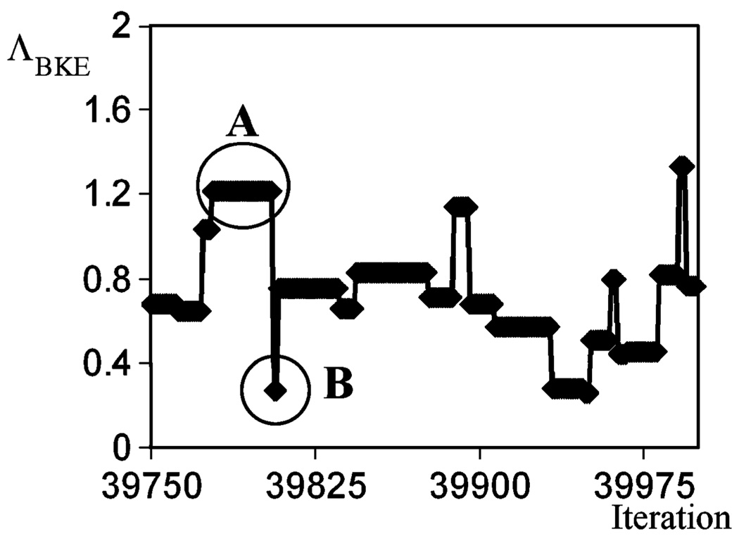
We generated one Markov Chain for a particular input projection image, g⃑, calculating the LR values over the region described above. As illustrated in Fig. 1, the output of the Markov chain is a series of θ⃑^(j) sampled from the posterior probability $\text{pr}(\stackrel{\rightharpoonup }{\theta }|\stackrel{\rightharpoonup }{g},H_0)$. Each θ⃑^(j) results in one corresponding ${\mathrm{\Lambda }}_{\text{BKE}}^{(j)}$. Fig. 4 shows the outputs ${\mathrm{\Lambda }}_{\text{BKE}}^{(j)}$ from a segment of the Markov chain corresponding to iterations, j = 39 750–40 000. In Fig. 4 we see that the plot of Λ_BKE versus iteration number has plateaus, such as the region A. The plateaus are the results of rejected proposals, where ${\mathrm{\Lambda }}_{\text{BKE}}^{(j)}$ remains unchanged. On the other hand, there are also sudden changes in the plot, e.g., region B. This corresponds to accepted proposals where the proposed background was accepted in the Markov chain, resulting in changes in the value of ${\mathrm{\Lambda }}_{\text{BKE}}^{(j)}$.

Fig. 4.

Segment of the Markov chain.

Burn-In Iterations

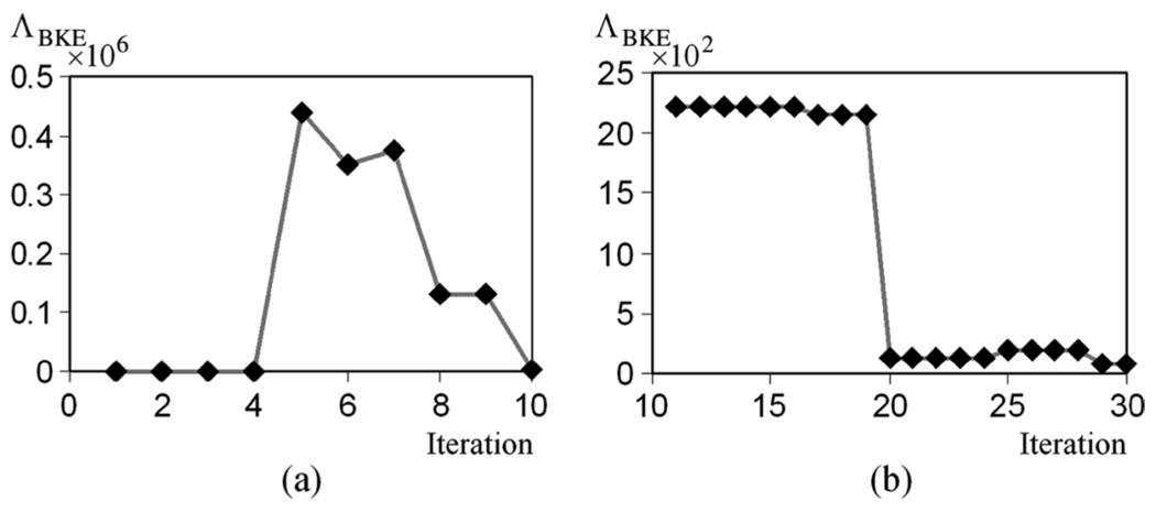
To start the Markov chain, an initial sample is required, as illustrated in Fig. 1. We chose to use the mean of each parameter, whose range is defined in Table I and Table II, to be the initial sample of this parameter. The choice of the initial sample biases the subsequent LRs, and the amount of bias decreases with iteration. An example of this phenomenon is shown in Fig. 5. This figure shows the Λ_BKE values obtained from [Fig. 5(a)] the first 10 iterations and (Fig. 5) 11–30 iterations of a Markov chain. Note that the vertical scales in these two graphs are quite different, suggesting the fluctuation of the unstabilized Markov chain.

Fig. 5.

Λ_BKE obtained (a) from the first 10 iterations, and (b) from the 11th to 30th iterations. Note that vertical scale is different for (a) and (b).

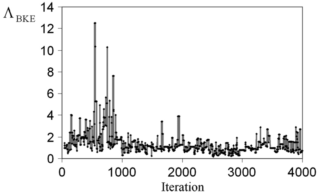
As a result of the bias, the early outputs of the chain are often discarded and not included in the sum of (4). These discarded iterations are referred to as burn-in iterations in the MCMC literature. Fig. 6 shows Λ_BKE values obtained from the 40–4000 iterations. It appears that, after 1000 iterations, the Markov chain obtained for this particular projection data stabilizes. To guarantee the stabilization of each Markov chain for the computation of Λ̂ for each projection data, we used 4 × 10⁵ burn-in iterations.

Fig. 6.

Λ_BKE evaluated at 40–4000 iterations. It can be seen that the Markov chain stabilizes after 1000 iterations.

Convergence of Λ̂ = Λ̂(g⃑)

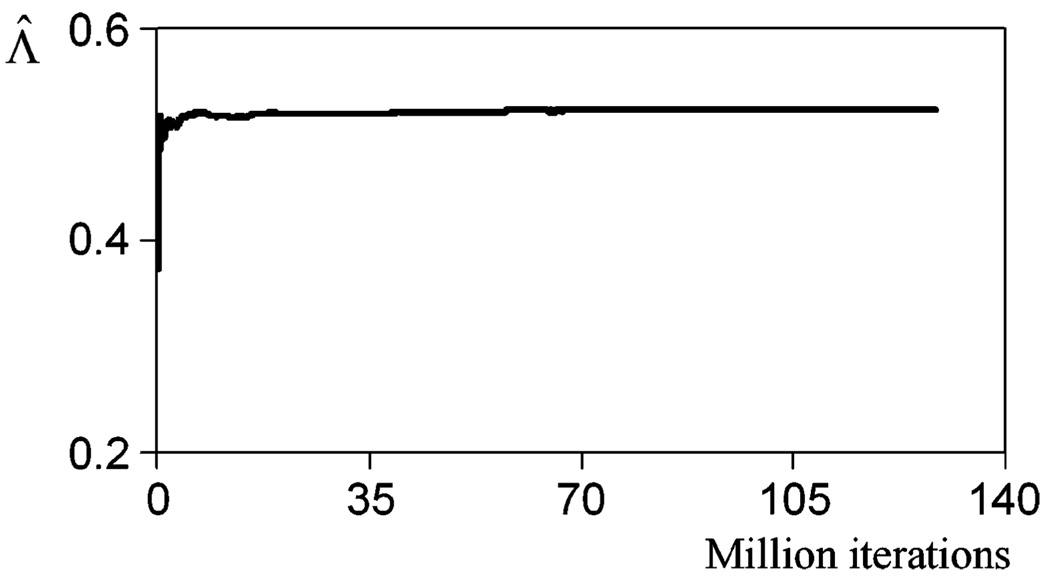
We plotted the estimated LR for this particular projection image Λ̂ versus iteration number, or the length of the Markov chain, as shown in Fig. 7, to demonstrate the convergence of Λ̂. A Markov chain of a total of 1.28 × 10⁸ iterations was generated. It can be seen in Fig. 7 that after 0.4 × 10⁸ iterations, Λ̂(g⃑) stabilizes. In the subsequent studies, we used 1.0 × 10⁸ iterations to compute Λ̂ for each projection image to ensure the convergence of the Markov chain. It took around 3 h to compute the Markov chain for each projection data to obtain one Λ̂, while without using this method, it would take around six years to generate one Λ̂.

Fig. 7.

Convergence of Λ̂ for a particular data vector g⃑.

Distribution of the Output of One Markov Chain

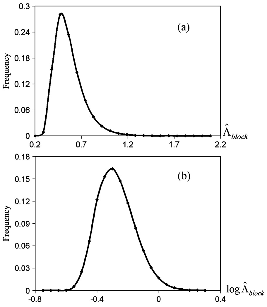
In MCMC, each output LR in the chain ${\mathrm{\Lambda }}_{\text{BKE}}^{(j)}$ is dependent on the previous ${\mathrm{\Lambda }}_{\text{BKE}}^{(j-1)}$. Thus, the outputs in the Markov chain are not independent and identically-distributed (i.i.d.). We divided the output into blocks; each block had 4000 iterations. We calculated the average LR in each block, denoted by Λ̅_block. The average LR of the ith block is expressed as Λ̅_block−i where i is the block number. It can be shown that breaking Markov chains into blocks is an effective technique for approximating i.i.d. variables, and allows for the computation of standard deviations [6]. Fig. 8(a) shows the histogram of Λ̅_block for this particular Markov chain, which resembles a log normal distribution, and Fig. 8(b) shows a histogram of the log Λ̅_block, which was approximately Gaussian distributed.

Fig. 8.

Histogram of (a) Λ̅_block and (b) log Λ̅_block.

B. Validating the MCMC IO Estimation Method Using the Properties of LR

Theoretically, the LR has the following properties for an ensemble of binary objects [7], e.g., the defect-present/absent images in our study

$$\begin{array}{cc}\langle \mathrm{\Lambda }|H_0\rangle \hfill & ={\displaystyle \underset{\infty }{\int }f(\stackrel{\rightharpoonup }{g}|H_0)\frac{f(\stackrel{\rightharpoonup }{g}|H_1)}{f(\stackrel{\rightharpoonup }{g}|H_0)}{d}^M\stackrel{\rightharpoonup }{g}}\hfill \\ \hfill & ={\displaystyle \underset{\infty }{\int }f(\stackrel{\rightharpoonup }{g}|H_1)d^M\stackrel{\rightharpoonup }{g}}\hfill \\ \hfill & =1\hfill \end{array}$$ (11)

and

$$\langle \mathrm{\Lambda }|H_1\rangle -\mathit{\text{Var}}(\mathrm{\Lambda }|H_0)=1$$ (12)

where (11) suggests the mean of Λ under the hypothesis is H₀ is 1, and (12) suggests the mean of Λ under hypothesis H₁ minus the variance of Λ under H₀ hypothesis is 1. Using these two properties, we can validate the IO estimation algorithm using a large number of samples.

The LR of an ROI can be viewed as the product of LR of each pixel in the ROI. According to the central limit theorem, LR is thus approximately log-normal distributed. Log-normal distribution is asymmetric. In this case, the theoretical mean of the LR under H₀ is 1.0. A LR estimate for a particular projection image Λ̂ that is close to zero might have the same probability as a LR that is large. In averaging the Λ̂ obtained from different projections images, a Λ̂ that is close to zero does not change the mean value much, while an Λ̂ that is large might significantly affect the mean value. Thus, a large number of samples are needed to demonstrate the properties in (11) and (12). In the presented study, 2000 pairs of images were used.

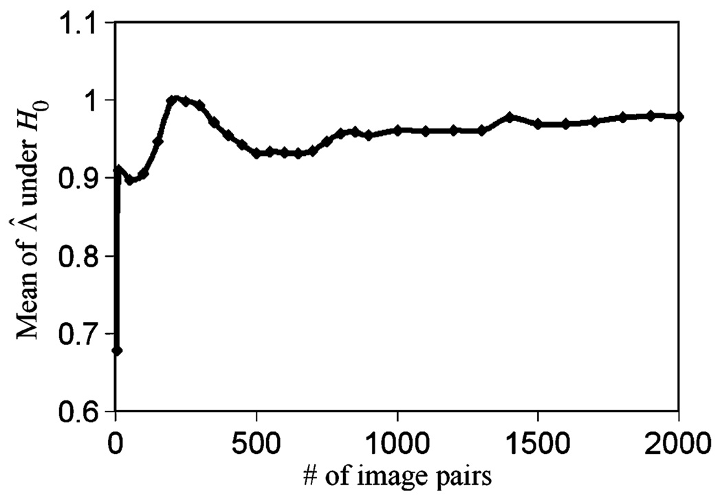
We first tested (11). Fig. 9 shows the convergence of 〈Λ̂|H₀〉 as a function of the number of sample projection pairs used. When the sample size was 2000 pairs, 〈Λ̂|H₀〉= 0.979, which is close to 1.0.

Fig. 9.

The convergence of 〈Λ̂|H₀〉.

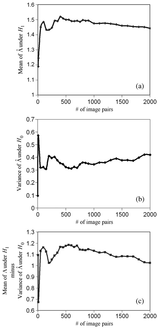
We then tested (12). Fig. 12(a) shows the convergence of 〈Λ̂|H₁〉, Fig. 12(b) shows the convergence of Var(Λ̂|H₀), and Fig. 12(c) shows the convergence of the estimation of 〈Λ̂|H₁〉 − Var(Λ̂|H₀). When the sample number reaches 2000 pairs, 〈Λ̂|H₁〉 − Var(Λ̂|H₀) converges to 1.026, which is very close to 1 as predicted theoretically in (10).

Fig. 12.

The convergence of 〈Λ̂|H₁〉 − Var(Λ̂|H₀).

C. Comparing IO and Hotelling Observer (HO) Performance

The purpose of this experiment was to compare the performance of IO obtained using the MCMC technique and that of the HO. Theoretically, IO outperforms HO in general. When the data follow multivariate Gaussian distribution with equal covariance, IO performance is identical to that of the HO.

Due to the difficulty in computing IO, the optimal linear observer HO is conventionally considered as an alternative in system optimization. The HO, however, is also very hard to compute. This is because the computation of HO requires the inversion of a covariance matrix. For an ensemble of images that has K elements each, the resulting covariance matrix has a dimension of K × K. In order to obtain an invertible covariance matrix, at least (K × K) + 1 images are required, and the inversion of a large matrix is usually inaccurate due to numerical errors [8]. For example, if the image dimension is 32 × 32, the inversion of a covariance matrix of 1024 × 1024 is needed to compute HO. In this work, we used a line ROI that has 44 pixels. The small data vector dimension results in a covariance matrix of 44 × 44 that can be easily inverted for HO calculation.

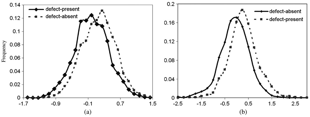
We first investigated the IO performance. Fig. 10 shows the histogram of Λ̂ of the 2000 pairs of images. Fig. 10(b) shows a magnification of Fig. 10(a) when the values of Λ̂ are less than 2.0. On Fig. 10, we see that the distribution of Λ̂ is asymmetric and is approaching a log-normal distribution.

Fig. 10.

The histogram of ideal observer likelihood ratios. The plot on the right expands the region indicated on the left by using 10 histogram bins (as opposed to two). In these plots, the points indicate the location of the histogram bin and the lines only represent a smooth curve drawn through the points.

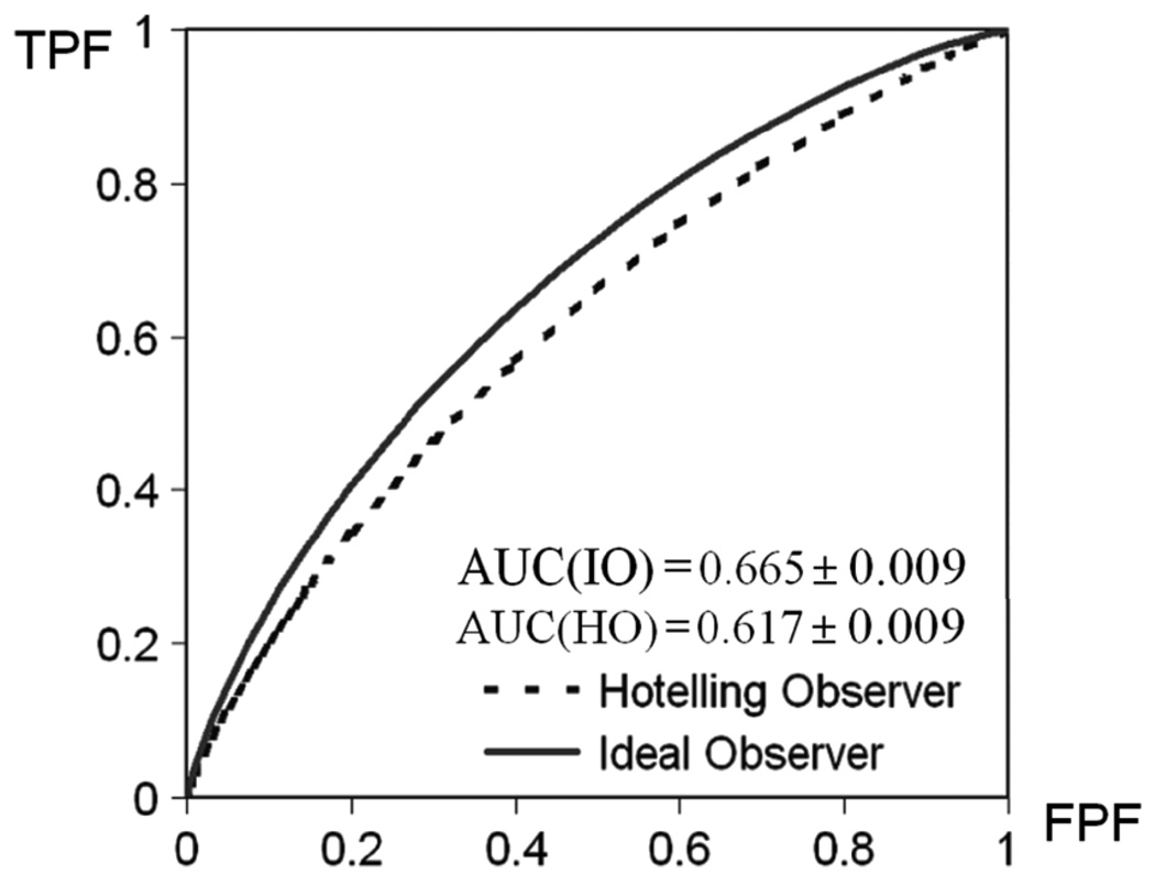
Fig. 11(b) shows the histogram of log Λ̂. It can be seen that the histograms of the defect-present and defect-absent distributions are overlapped, the shape of the distributions are approximately Gaussian. The ROC curve of the IO is shown in Fig. 13.

Fig. 11.

(a) Histograms of Hotelling observer test statistics. (b) Histograms of IO test statistic, log Λ̂, of the two classes.

Fig. 13.

ROC curves of the two observers. The ROC curve of IO is uniformly better than that of the HO.

Theoretically, IO uses LR as the optimal decision variable. LR has been proved to be the optimal decision variable that provides the highest area under the curve (AUC) value. In Fig. 13, the IO achieves a uniformly higher ROC curve than the Hotelling observer, as predicted. In particular, the AUC value for the IO was 0.665 ± 0.009, and that for the HO was AUC = 0.617 ± 0.009. The ROC curves and the AUC values were obtained using software LABROC4 [9] which do not assume that the input test statistics are normally distributed.

D. Properties of the Moment Generating Function and AUC Value Estimated Using the Likelihood Generating Function

The moment-generating function for λ under hypothesis H₀ is given in [10] and expressed as

$$M_0(\beta )={\displaystyle \underset{0}{\overset{\infty }{\int }}}{\mathrm{\Lambda }}^{\beta }\text{pr}(\mathrm{\Lambda }|H_0)d\mathrm{\Lambda }={\langle {\mathrm{\Lambda }}^{\beta }\rangle }_0$$ (13)

where β is any real constant. Reference [10] also gives the likelihood generating function, G(β), given by

$$M_0(\beta )=\text{exp}[\beta (\beta -1)G(\beta -0.5)].$$ (14)

The IO AUC can be estimated from G(0)

$$2(1-{\mathit{\text{AUC}}}_{\mathrm{\Lambda }})\approx 1-\text{erf}\left\{{\left[\frac{1}{2}G(0)\right]}^{\frac{1}{2}}\right\}.$$ (15)

A number of references have shown the accuracy of (15) in estimating the AUC value [10], [11].

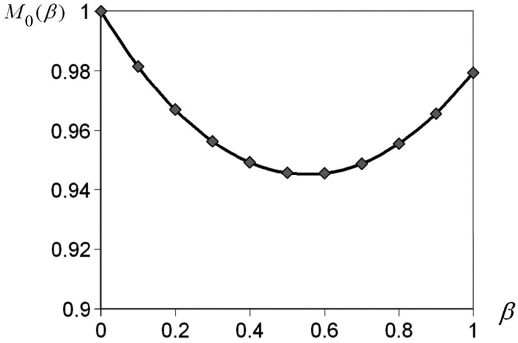
From (14), we see that the theoretical prediction of M₀(β) is a quadratic function of β. We thus computed M₀(β) using (13) and plotted it as a function of β to test whether the experimentally obtained moments agreed with theoretical predictions. The results are shown in Fig. 14. It can be seen that the curve has the expected quadratic shape and is very close to (1.0,1.0) at the right endpoint.

Fig. 14.

Plot of M₀(β) as a function of β. The curve has the expected quadratic shape and passes very close to the point (1.0, 1.0) at the right endpoint.

We also checked the approximation in (15) to see if it holds in this experiment.We substituted the experimental value for G(0) into (15), and the resulting AUC value was 0.682, which is close to the AUC value obtained in Section II-C, 0.665.

III. DISSCUSSION

In this study we demonstrated the feasibility of the application of MCMC to IO estimation for a realistic SPECT projector and a parameterized phantom. To perform a comprehensive IO evaluation and optimization study for cardiac SPECT, a number of practical issues need to be addressed to achieve an appropriate compromise between computation time and realism. We briefly discuss these issues in the following.

Number of Anatomic Parameters and Their Discretization

In this study, we used two anatomic parameters to define the phantom. For a more realistic evaluation study, more anatomic parameters are needed. Increasing the number of anatomic parameters will dramatically increase the size of the database after parameter discretization. For example, for a phantom where three parameters are used to define the sizes of the heart, body and lung, the discretization will result M in hearts, N bodies, and K lungs. Thus the total number of anatomies in the database will be M × N × K, resulting in a database that is K times larger than the two-parameter database. When performing the MCMC IO estimation, having a database of phantom projections that can be loaded into main memory dramatically increases the speed of MCMC IO estimation. As a result, a larger database requires either more computer memory or moving the database to disk and accepting the resulting reduction in the speed of MCMC IO estimation.

Another important issue regarding the anatomic parameter discretization is the number of samples to be used in the database, e.g., the number of heart sizes M and the number of body sizes N. We chose M = N = 50 in this work with the purpose of maintaining a small database for this is a feasibility study. Increasing the number of samples would provide a better approximation of the true continuous distribution. As a result, the estimated LR should approach that obtained from continuous anatomic parameter distributions as we increase the number of discretized samples. However, increasing the number of samples also increases the size of the database. An important issue is how many samples are sufficient. Our hypothesis is that increasing the number of (or decreasing the spacing between the) samples will result in estimated LRs that are the same as those from the continuous distribution when the spacing is significantly smaller than that of the system resolution. An investigation of this is an important topic for future work.

Burn-In Iterations and Stopping Criterion for the Markov Chain

Both the number of burn-in iterations and the stopping criterion affect the accuracy of the IO performance estimate. In this study, we first identified empirical values for the number of burn-in iterations and the total number of iterations, and then used more than enough burn-in and stopping iterations to ensure the convergence of Markov chain. Developing an adaptive criterion to identify the number of burn-in and total iterations adaptively, for example based on a threshold on an estimate of the variance of the Markov chain output of the Markov chain, would improve the efficiency of the method.

Ideal Observer and Hotelling Observer Performance

This paper describes a new method to allow faster estimation of IO performance based on a fast implementation of MCMC techniques. Even using the proposed method, the computational requirements are still large. In many cases where only the rankings of methods are needed, other observers, such as the HO, may be sufficient. However, before using these observers, it is desirable to demonstrate that rankings produced by them and the IO are consistent. In some cases, theoretical considerations may be sufficient; in other cases, the proposed method may allow empirical demonstration that this is the case.

IV. CONCLUSION AND FUTURE WORK

We applied Kupinski’s MCMC IO estimation technique to estimate the IO test statistic in cardiac SPECT imaging using a parameterized torso phantom and a realistic analytical SPECT projector. We then validated the proposed IO estimation technique by computing values of the IO test statistic for a large number of input images. The properties of these test statistics agreed well with the theoretical predictions and the ROC curve for the IO is everywhere higher than the ROC curve for the HO. This method is developed for SPECT imaging. However, it can be adapted to any linear imaging system.

In the future, we will apply this method to investigate several aspects of MPS imaging. First, variations in perfusion defects, i.e., signal variability [12], will be investigated. Second, a more realistic phantom model, e.g., the 4-D NCAT phantom [13], will be employed. Third, more realistic SPECT simulation tools, e.g., a fast MC-based simulation code, will be used to generate the organ projections. In addition, we will incorporate the MCMC IO estimation technique and the newly developed three-class ROC methodology [14]–[16] to develop three-class IO estimation techniques for the optimization of energy windows in simultaneous acquisition dual-isotope MPS imaging.

REFERENCES

- 1.Kupinski MA, Hoppin JW, Clarkson E, Barrett HH. Ideal-observer computation in medical imaging with use of Markov-chain Monte Carlo techniques. J. Optical Soc. Amer. A, Opt. Image Sci. Vis. 2003;vol. 20:430–438. doi: 10.1364/josaa.20.000430. [DOI] [PMC free article] [PubMed] [Google Scholar]
- 2.Rolland JP, Barrett HH. Effect of random background inhomogeneity on observer detection performance. J. Opt. Soc. Amer. A, Opt. Image Sci. Vis. 1992;vol. 9:649–658. doi: 10.1364/josaa.9.000649. [DOI] [PubMed] [Google Scholar]
- 3.Gross KA, Kupinski MA, Hesterman JY. A fast model of a multiple-pinhole SPECT imaging system. presented at the SPIE Med. Imag. Conf.; San Diego, CA. 2005. [Google Scholar]
- 4.Gross KA, Kupinski MA, Peterson TE, Clarkson E. Optimizing a multiple-pinhole SPECT system using the ideal observer. presented at the SPIE Med. Imag.; San Diego, CA. 2003. [Google Scholar]
- 5.Metropolis N, Rosenbluth AW, Rosenbluth MN, Teller AH, Teller E. Equation of state calculations by fast computing machines. J. Chem. Phys. 1953;vol. 21:1087–1092. [Google Scholar]
- 6.Jones GL, Haran M, Caffo BS, Neath R. Fixed-width output analysis for Markov chain Monte Carlo. J. Amer. Stat. Assoc. 2006;vol. 101:1537–1547. [Google Scholar]
- 7.Barrett HH, Myers KJ. Foundations of Image Science. New York: Wiley; 2003. [Google Scholar]
- 8.Fukunaga K, Hayes RR. Effects of sample-size in classifier design. IEEE Trans. Pattern Anal. Mach. Intell. 1989 Aug;vol. 11(no. 8):873–885. [Google Scholar]
- 9.Metz CE. LABROC4. Chicago, IL: Univ. Chicago; 1993. [Google Scholar]
- 10.Clarkson E, Kupinski MA, Hoppin JW. Assessing the accuracy of estimates of the likelihood ratio. presented at the SPIE Med. Imag.; San Diego, CA. 2003. [Google Scholar]
- 11.Clarkson E, Barrett HH. Approximations to ideal-observer performance on signal-detection tasks. Appl. Opt. 2000;vol. 39:1783–1793. doi: 10.1364/ao.39.001783. [DOI] [PubMed] [Google Scholar]
- 12.Park S, Kupinski MA, Clarkson E, Barrett HH. Ideal-observer performance under signal and background uncertainty. Proc. Inf. Process. Med. Imag. 2003;vol. 2732:342–353. doi: 10.1007/978-3-540-45087-0_29. [DOI] [PubMed] [Google Scholar]
- 13.Segars WP, Tsui BM, Lalush DS, Frey EC, King MA, Manocha D. Development and application of the new dynamic Nurbs-based Cardiac-Torso (NCAT) phantom. J. Nucl. Med. 2001;vol. 42:7. [Google Scholar]
- 14.He X, Frey EC. An optimal three-class linear observer derived from decision theory. IEEE Trans. Med Imag. 2007 Jan;vol. 26(no. 1):77–83. doi: 10.1109/TMI.2006.885335. [DOI] [PubMed] [Google Scholar]
- 15.He X, Metz CE, Tsui BMW, Links JM, Frey EC. Three-class ROC analysis—A decision theoretic approach under the ideal observer framework. IEEE Trans. Med. Imag. 2006 May;vol. 25(no. 5):571–581. doi: 10.1109/tmi.2006.871416. [DOI] [PubMed] [Google Scholar]
- 16.He X, Frey EC. Three-class ROC analysis—The equal error utility assumption and the optimality of three-class ROC surface using the ideal observer. IEEE Trans. Med. Imag. 2006;vol. 25:979–986. doi: 10.1109/tmi.2006.877090. [DOI] [PubMed] [Google Scholar]