The automatic detection of the optic disc location in retinal images using optic disc location regression

Abstract

The automatic detection of the position of the optic disc is an important step in the automatic analysis of retinal images. A method to detect the approximate position of the optic disc using kNN regression is presented. The method starts by building a regression model of the optic disc position. Using a prior vessel segmentation all vessel pixels are searched for those which are inside the optic disc according to the regression model. The regression output is blurred to handle noise. The point which is closest to the middle of the optic disc is chosen. The method was tested on 1000 screening images and was able to find the correct position in 99.9% of all cases.

I. INTRODUCTION

Diabetic retinopathy is the primary cause of visual loss and blindness in the working population in the United States and Europe. Early diagnosis and treatment has been shown to prevent this. Computer diagnosis is called for to allow detection of early signs of diabetic retinopathy in 18 million patients with diabetes every year[1][6]. In programs for early diagnosis, less than 10more than 90

Disc localization is an important aspect of computer diagnosis for determining whether the images are from a left or right eye, and for determining the relevance of potential lesions. Previous algorithms on disc localization have been published [3]. An elegant unsupervised solution was recently proposed by Foracchia et al., based on the shape of the vessel arch [4]. These algorithms were tested on the ‘Hoover set’[3] a test sets with pathology based on images used in the clinic. The advantage of these approaches and the test set used is that the robustness of the algorithm with respect to image perturbations by hemorraghes, exudates and other lesions can be established. However, in early diagnosis images with pathology would be rejected anyway, and for the purpose of early diagnosis in large image sets, validity of the algorithm on large datasets may be more important than robustness[2]. In this paper, we have developed a simple and elegant supervised method to detect the location of the optic disc in retinal images with few or no abnormalities. The vessels and the pixel intensities are used as the parameters for a distance regression model.

The vessel orientation, width and density in a local area on the retina provide information about our position on the retina. In general, the closer one comes to the optic disc the wider and denser the vessels become. Foracchia et al. used the global orientation of the vasculature to find the position of the optical disc. Locally, the orientation of the vasculature also gives information concerning the position on the retina.

In the approach presented in this work we use kNN regression to find the relationship between the dependent variable d, the distance to the optic disc center, and a feature vector measured under and around a circular template. We propose a set of features which could possibly be useful to do the regression.

II. MATERIALS

A total of 1100 retinal images were used in this research. All images were anonimized and the study was performed according to the guidelines set forth in the Declaration of Helsinki. No personalized Health Information was accessible to the researchers. The training images, 100 in total, and the test images, 1000 in total, were acquired from screening programs in the Netherlands[1]. Primary care patients with diabetes for diabetic retinopathy are screened in family care physician’s offices or family physician laboratories. The images, all JPEG compressed, were obtained at twenty different sites. Each of the images was resized such that their circular Field of View (FOV) had the same diameter, 540 pixels in diameter. Three different camera types were used: the Topcon NW 100 and NW 200 (Topcon, Tokyo, Japan) and the Canon CR5-45NM (Canon, Tokyo, Japan). The second author marked all optic disc center locations in every image in the training set, supervised by the first author, a retinal specialist. Two independent observers indicated the optic disc center location and the optic disc border for all images in the test set. In this case, the first observer was selected as the reference standard.

III. METHODS

A. The Optic Disc Distance Regression Model

We want to find the position in the image which is located in the middle of the optic disc. To accomplish this we will use kNN regression [5] to find the relationship between the dependent variable d, representing the distance to the optic disc center, and a feature vector measured around a circular template. The template is circular because the optic disc is approximately circular itself. The circular template is placed at various locations in the image and measure the features around the template. Based on the feature vector the distance between the center of the template and the center of the optic disc is estimated. The template itself is divided into 4 sections (see Figure 1). The template radius r is a free parameter which should be set during training. We measure a number of features at each piece as well as some features for the entire template. These features consist of:

1. Number of vessels.

2. Average vessel width.

3. Standard Deviation of the Vessel width.

4. Average vessel orientation.

5. Standard Deviation of the vessel orientation.

6. Maximum vessel width.

7. Maximum width vessel orientation.

8. Average intensity (green plane) under the template.

9. Standard deviation of the intensity (green plane) under the template.

10. Average Vessel width under the template.

11. Number of vessel pixels under the template.

Features 1-7 are measured for each template piece and features 8-11 are measured once for the entire template. The entire measured feature vector thus consists of 32 features.

Fig. 1.

The circular template, divided into 4 equal quadrants. The dot on the template border is the point where feature measurement starts. The radius r of the template is a free parameter.

B. Vessel segmentation and analysis

In order to measure some of the features around the template we need a segmentation and analysis of the vasculature. To accomplish this, a previously presented pixel classification based approach was used [6]. This supervised approach was trained using a set of images in which all vasculature had been segmented, the DRIVE database [7]. A posterior probability map was produced which indicates, for each pixel in the field of view, the probability that a pixel is a vessel pixel. By thresholding this map a binary vessel segmentation was produced. To measure the orientation of the vasculature the vessel centerlines are determined by thinning the binary segmentation [8]. Next, individual vessel segments were found by removing all vessel bifurcations and crossings. This was necessary as the vessel orientation and width is not well defined in these points. Bifurcations and vessel crossings were removed by removing all pixels from the thinned image which have more than two neighbors.

First the local orientation of each vessel segment was determined by selecting, in turn, each centerline pixel and its 3 neighbors to both sides (if available) and applying Principal Component Analysis on their coordinates. The direction of the largest eigenvector of the covariance matrix is the local orientation.

To measure the width of the vasculature for each centerline pixel, the local orientation was used. Perpendicular to this orientation, the distance from the centerline pixel to the edge of the vessel in the posterior probability map as produced by the vessel segmentation was measured.

C. Feature Measurement

Once the segmentation and analysis of the vasculature has been completed we can measure the previously mentioned features everywhere in the image. To measure features 1-7 we traversed the circular template starting at the position marked with the dot in Figure 1 and proceed along the template border in a clockwise fashion. When a centerline pixel is encountered, which is not part of a vessel segment previously encountered, this is counted as one vessel found in a certain quadrant. The vessel width and orientation were recorded as well. After a quadrant was completed, the vessel widths and orientations were averaged and their standard deviation was calculated. Finally, the width and orientation of the widest vessel for this quadrant was stored. When this was done for all quadrants the average pixel intensity of the green image plane under the template and the standard deviation of the pixel intensities was measured. The average vessel width was determined by dividing the total number of vessel pixels under the template by the number of centerline pixels.

D. Training the System

Training the system was done by applying the vessel segmentation and analysis to all images in the training set. Then, every tenth pixel in a rectangular grid centered on the optic disc center and of size 2r squared was sampled. This was implemented by centering the circular template on a certain pixel and extracting the features. Each feature vector was stored together with a value d, the distance to the optic disc center. After the entire grid was sampled a number (for the present system, 200) of randomly selected different locations in the image are also sampled. The maximum distance d to the optic disc center was limited to the value of r as it is unlikely the system is able to estimate a distance much larger than r. The complete set of samples for all training images formed the training dataset. Before the training set can be used all features were normalized to unit standard deviation. The training set can then be used in the final system to estimate the distance from any location in the image to the optic disc center.

To estimate the distance d to the optic disc center given a feature vector, the k=11 nearest neighbors in the feature space are found and the values d of these nearest neighbors are averaged. This average value is returned as the estimate of d. The value of k=11 was empirically determined using the training set.

E. Feature Selection

The complete set of features is not necessarily the optimal set of features to give the best regression results. By applying a feature selection method overall system performance can be improved. A supervised feature selection method was applied, called Sequential Floating Feature Selection [9]. The algorithm employs a “plus 1, take away i” strategy. In other words, the algorithm adds features to an empty feature set and removes features if that improves the overall performance. In this way “nested” groups of good features can be found. Performance in this case was measured as the minimum average regression distance. As the feature selection is supervised the training set was randomly divided into a feature selection training and test set.

After feature selection the following features were selected. The number of vessels, as well as the orientation of the widest vessel, were selected in every quadrant, resulting in 8 features. For the whole template, the average and standard deviation of the image intensity under the template as well as the average vessel width and number of vessel pixels was selected. The total number of features used in the system was 12.

F. Applying the System

To find the optic disc center we searched all pixels that are part of a vessel as indicated by the vessel segmentation. For every vessel pixel the distance d to the optic disc center was determined. Because the highest value returned by the regression is r, the distances for all pixels, not part of a vessel, are set to r. Next the image is blurred, with a Gaussian kernel with σ = 15. This value was determined empirically, but does not have a large influence on the final result of the method. Finally we found the pixel with the lowest value in the image and selected that pixel as the optic disc center location. See also Figure 2,3,4 and 5.

Fig. 2.

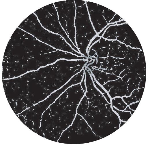
The intensities of the vessel pixels in this image indicate the distance from the optic disc center. As the maximum distance is equal to radius r of the circular template, pixels further than r pixels away from the optic disc have the same value.

Fig. 3.

Here all background pixels have been given the value r. The pixels with lower values, i.e. close to the optic disc center, stand out.

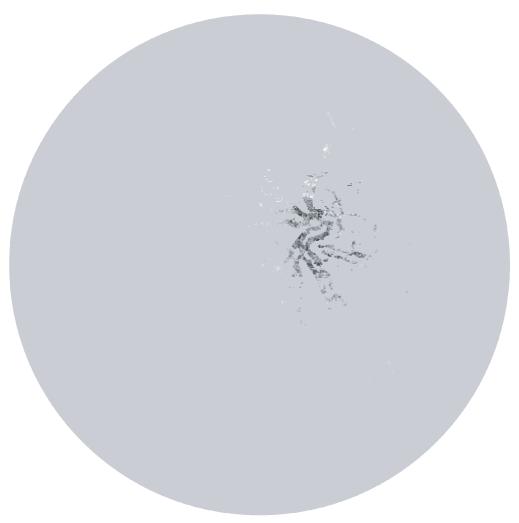
Fig. 4.

After blurring, a dark spot on top of the optic disc remains. The lowest value in this spot is selected as the optic disc center.

Fig. 5.

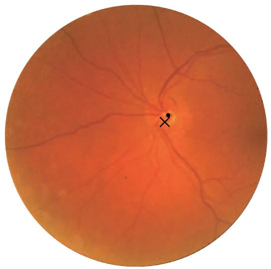
An example result; the cross indicates the optic disc center found by the system and the dot indicates the center indicated in the reference standard.

IV. EXPERIMENTS AND RESULTS

The system was applied to all 1000 images in the test set. Parameter r was chosen as 50 pixels, which makes the template a little larger than the average optic disc diameter of around 80. The system was able to find the correct position, i.e. a position within the optic disc border as indicated by the reference standard, in 99.9% of all cases. The average distance of the found optic disc center to the real optic disc center was 9.75 pixels with a standard deviation of 16.14 pixels. The second human observer was able to find the optic disc center in 100% of all cases. Average time was 1 minute, 30 seconds for the vessel segmentation and 30 seconds for the analysis.

V. CONCLUSION

The results indicate that a simple and elegant supervised algorithm, optic disc location regression, is valid. It is capable of finding the correct location, based on the reference standard, of the optic disc in over 999 out of 1000 retinal images, with pathology in 10% of them. These results indicate that this novel approach has the potential to detect the location of the optic disc in retinal images with few or no abnormalities. In the images where it failed, it failed because of a failedg vessel segmentation, usually due to low contrast. Compared to the approaches by Hoover and Foracchia[3][4], which are more robust, this algorithm has the advantage that it is fast (30s) and easier to optimize. Remember that for computer diagnosis of these images, vessel segmentation is a first step, so that the time needed to segment the vessels can be discounted[2]. In addition, a failure of the algorithm may be one of the criteria that helps to decide that that image is not suitable for computer diagnosis. In summary, we propose optic disc location regression as an interesting approach for fast optic disc location in fundus color images that are obtained in early diagnosis and screening projects.

REFERENCES

- [1].Abràmoff MD, Suttorp M. Web-based screening for diabetic retinopathy in a primary care population: the Eye Check project. Telemedicine and e-Health. 2005;11(6) doi: 10.1089/tmj.2005.11.668. [DOI] [PubMed] [Google Scholar]
- [2].Niemeijer M, van Ginneken B, Staal JJ, Suttorp-Schulten MSA, Abràmoff MD. Automatic Detection of Red Lesions in Digital Color Fundus Photographs. IEEE Transactions on Medical Imaging. 2005;24:584–592. doi: 10.1109/TMI.2005.843738. [DOI] [PubMed] [Google Scholar]
- [3].Hoover A, Goldbaum M. Locating the Optic Nerve in a Retinal Image Using the Fuzzy Convergence of the Blood Vessels. IEEE Transactions on Medical Imaging. 2003;22:951–958. doi: 10.1109/TMI.2003.815900. [DOI] [PubMed] [Google Scholar]
- [4].Foracchia M, Grisan E, Ruggeri A. Detection of Optic Disk in Retinal Images by Means of a Geometrical Model of Vessel Structure. IEEE Transactions on Medical Imaging. 2004;23:1189–1195. doi: 10.1109/TMI.2004.829331. [DOI] [PubMed] [Google Scholar]
- [5].Duda R, Hart P, Stork D. Pattern classification. John Wiley and Sons; New York: 2001. [Google Scholar]
- [6].Niemeijer M, Staal J, van Ginneken B, Loog M, Abràmoff M. Comparative study of retinal vessel segmentation methods on a new publicly available database. SPIE Medical Imaging. 2004;5370:648–656. [Google Scholar]
- [7].Staal J, Abràmoff M, Niemeijer M, Viergever M, van Ginneken B. Ridge based vessel segmentation in color image of the retina. IEEE Transactions on Medical Imaging. 2004;23(4):501–509. doi: 10.1109/TMI.2004.825627. [DOI] [PubMed] [Google Scholar]
- [8].Eberly D. Skeletonization of 2d binary images. 2001 http://www.magic-software.com/Documentation/Skeletons.pdf.
- [9].Pudil P, Novovicova J, Kittler J. Floating search methods in feature selection. Pattern Recognition Letters. 1994;15(11):1119–1125. [Google Scholar]