Cluster Mass Inference via Random Field Theory

Abstract

Cluster extent and voxel intensity are two widely used statistics in neuroimaging inference. Cluster extent is sensitive to spatially extended signals while voxel intensity is better for intense but focal signals. In order to leverage strength from both statistics, several nonparametric permutation methods have been proposed to combine the two methods. Simulation studies have shown that of the different cluster permutation methods, the cluster mass statistic is generally the best. However, to date, there is no parametric cluster mass inference method available. In this paper, we propose a cluster mass inference method based on random field theory (RFT). We develop this method for Gaussian images, evaluate it on Gaussian and Gaussianized t-statistic images and investigate its statistical properties via simulation studies and real data. Simulation results show that the method is valid under the null hypothesis and demonstrate that it can be more powerful than the cluster extent inference method. Further, analyses with a single-subject and a group fMRI dataset demonstrate better power than traditional cluster extent inference, and good accuracy relative to a gold-standard permutation test.

1 Introduction

Cluster extent and voxel intensity are two widely used statistics in neuroimaging inference. Cluster extent is sensitive to spatially extended signals [7, 23], while voxel intensity is sensitive to focal, intense signals [6, 25]. Both can suffer from a lack of power for signals of moderate extent and intensity [11]. Furthermore, one does not generally know, a priori, whether the generated signal is large in extent, intensity or both. While some practitioners simply select the statistic that gives the most statistically significant test, this embodies a multiple testing problem and will result in inflated false positive error rates. An ideal test statistic would combine spatial extent and peak height intensity and would be sensitive to both without increasing the number of tests considered.

Poline et al. [23] (henceforth referred to as PWEF) developed a method which combines extent and intensity based on Gaussian random field theory (RFT). They derived the joint distribution of cluster extent and voxel-wise peak height intensity and made inference on minimum P value of a cluster extent test and a local maximum intensity test. However, their method is only applicable to Gaussian or approximately Gaussian images (e.g. a very large group analysis, or a single subject fMRI analysis).

Cluster mass, the integral of suprathreshold intensities within a cluster, naturally combines both signal extent and signal intensity. Initially suggested by Holmes [13], he only provided the mean of cluster mass to the power 2/(D+2) for Gaussian field, where D is dimension. In addition, Bullmore et al. [2] used permutation to obtain cluster mass P values. Currently the cluster mass is the default test statistic in the BAMM¹ and CAMBA² software, and is implemented in FSL’s randomise³ tool and in the SnPM⁴ toolbox for SPM⁵.

Hayasaka & Nichols [11] studied the statistical properties of cluster mass along with a variety of other “combining methods” in the permutation testing framework. Among the combining methods they considered were Tippet’s method [16, 22] (minimum P values, used by PWEF) and Fisher’s method (−2 × sum of ln P values). Through simulation studies and analyses of real data they concluded that the nonparametric cluster mass method is generally more powerful than other methods they investigated.

A strength of nonparametric inference methods is that they rely on fewer assumptions about the distributional form of the data. However, they require additional computational effort and are not very flexible. For example, the precise permutation scheme used depends on the experimental design and cannot be trivially determined from a design matrix. Nuisance covariates cannot be accommodated in general, as they induce null-hypothesis structure which violates exchangeability. Also, nonparametric methods cannot be used directly for single subject data analysis as a parametric autocorrelation model or wavelet transformation is needed to whiten the data. For all of these reasons, a parametric cluster mass inference method that can operate with a general linear model and deal with single subject analyses would be of great value.

In this paper we develop a theoretical distribution for the cluster mass statistic via Gaussian RFT. We generalize the work of PWEF, deriving the cluster mass statistic, extending the method to Gaussianized t data. We study the statistical size and power of our test on Gaussian and Gaussianized t image data through simulations and illustrate the method on two real data examples, a single subject fMRI dataset and a group level fMRI data analysis with low degrees of freedom.

2 Materials and Methods

2.1 Cluster mass test theory

In a mass univariate data analysis, a general linear regression model (GLM)

$$Y_i=X{\beta }_i+{\epsilon }_i$$ (1)

is fit for each voxel i = 1,…, I, where Y_i is an N × 1 vector of responses, X is a common N × q design matrix of predictors, β_i is a q × 1 vector of unknown parameters and ε_i is a N × 1 vector of random errors. Typically, at each voxel, errors are assumed to be independent and identically distributed $N(0,{\sigma }_i^2)$ random variates, though dependent errors can be accommodated [17]. The ordinary least squares estimator of β_i is β̂_i = (X^TX)⁻¹X^TY_i, and of ${\sigma }_i^2$ is ${\widehat{\sigma }}_i^2=e_i^{\mathrm{T}}{e}_i/\eta$, where e_i = Y_i − Xβ̂_i and where η is the error degrees of freedom. Then the Student’s t-statistic at voxel i is

$$T_i=c{\widehat{\beta }}_i{\left(c{(X^{\mathrm{T}}X)}^{-1}{c}^{\mathrm{T}}\widehat{{\sigma }_i^2}\right)}^{-1/2}$$ (2)

where c is a contrast of interest (row vector). We write the t-statistic image as $\mathbf{T}={\{T_i\}}_{i=1}^I$.

Given cluster-forming threshold u_c > 0, the set of suprathreshold statistics ${\{T_i:T_i>u_c\}}_{i=1}^I$ is used to define clusters. Contiguous clusters are defined by a neighborhood scheme, typically 18 connectivity scheme on a three dimensional image.

Let L be the number of clusters found, with cluster ℓ having S_ℓ, voxels (i.e. the cluster extent), ℓ = 1,2,…, L. Further let I_ℓ be the set of voxel indices corresponding to cluster ℓ. The cluster mass, M_ℓ, of cluster ℓ is the summation of the suprathreshold intensities:

$$M_{\ell }={\displaystyle \sum _{i\in I_{\ell }}{H}_i}$$ (3)

where H_i = T_i – u_c. Note that M_ℓ = S_ℓH̄_ℓ where H̄_ℓ = ∈_i∑Iℓ H_i/S_ℓ is the average suprathreshold intensity of cluster ℓ, showing cluster mass to be the product of the cluster extent and the average suprathreshold intensity.

To use Random Field Theory results, we begin by assuming that the standardized error images, called the component fields, are discrete samplings of a continuous, smooth, stationary Gaussian random process. The component field for scan j is {ε_ij/σ_i}_i, where ε_ij is the error for scan j at voxel i. The component fields are assumed to follow a mean zero, unit variance multivariate Gaussian distribution. Stationarity implies that the spatial correlation is determined by an auto-correlation function that is homogeneous over space. The process is regarded as “smooth” if the autocorrelation function has two derivatives at the origin. Based on these assumptions, the t image defined by (2) defines a Student’s t random field.

While any univariate random variable can be transformed into a Gaussian variate, or Gaussianized, a Gaussianized t image may not resemble a realization of Gaussian random field. Randomness in ${\widehat{\sigma }}_i^2$ reduces the smoothness of the statistic image relative to the component fields [25], as reviewed in Appendix B.7. However, Worsley et al [26] argues that when the t degrees of freedom exceed 120, the Gaussianized t-statistic can be regarded as a Gaussian Random Field. Hence we proceed by deriving results assuming T is a Gaussian image, but later return to the issue of Gaussianization.

The full derivation of our null distribution of the cluster mass statistic is given in Appendix B, but we sketch an overview of the result here. The derivation starts by approximating the statistic image about a local maximum as a paraboloid, which allows cluster mass to be obtained a function of cluster extent, S_ℓ, and suprathreshold peak intensity, H_ℓ = max{H_i : j ∈ I_ℓ},

$$M_{\ell }\approx 2/(D+2)\times S_{\ell }\times H_{\ell }$$ (4)

where D is the dimension of the image. While this parabolic approximation is essential to the derivation of the null distribution of M_ℓ, note we do not actually fit paraboloids to the image, and the test statistic computed from the data is exactly as specified in Eq. (3). By assuming that the autocorrelation function of the image is proportional to a Gaussian probability density function, the distribution of M_ℓ conditional on H_ℓ can be found. We follow PWEF, making a small excursion assumption that replaces peak height u_c + H_ℓ with u_c, creating what we denote the 𝒰 result, but also repeat the derivation without this assumption, deriving the Ƶ result.

Finding the joint distribution of (M_ℓ, H_ℓ) and integrating out H_ℓ yields the final result, an expression for P(M_ℓ > m), the uncorrected P-value for an observed cluster mass value of m. This requires two numerical integrations, one dependent on u_c, and one on m. In practice, for any given dataset, P-values for a grid m values can be pre-computed and interpolation used to find the P-value for an arbitrary value of m.

This theoretical approach also produces a new result for cluster extent S_ℓ, distinct from the original ([6]) result, which we also evaluate for completeness.

As P(M_ℓ > m) is an uncorrected P-value which does not account for searching over all clusters in the image, it is only appropriate for a single cluster that can be pre-identified before observing the data [5], a situation that rarely arises in practice. As detailed in Appendix B, the uncorrected P-values can be transformed into familywise-error corrected P-values which accounts for the chance of one or more false positive clusters anywhere in the image.

2.1.1 Student’s t-statistic image

As discussed above, when the degrees of freedom are small a Gaussian random field will not provide a good approximation for a Student’s t-statistic image. In such cases we Gaussianize the t image via the probability integral transform. The transformed image, however, will be rougher than the component fields, and so the roughness parameter must be adjusted according to the degrees of freedom of the t-statistic image. Thus we can apply our method to Gaussianized t images with just a modification to the smoothness estimate, as described in Appendix B.7.

2.2 Simulations

To evaluate the accuracy of our cluster mass result, Equation (4), both 2D (256 × 256) and 3D (64 × 64 × 30) Gaussian noise images are simulated. In order to understand the influence of image roughness on the proposed statistic, each of the 10,000 independent Gaussian noise images are convolved with different isotropic Gaussian smoothing kernels. Kernel sizes 2, 4, 8, 10, and 12 voxels full width at half maximum (FWHM⁶) are used, and these sizes then directly determine |Λ|, the image roughness parameter. Two cluster forming thresholds are investigated (U_c = 2.326 and U_c = 3.090, corresponding to uncorrected P = 0.01 and P = 0.001, respectively). A nominal significance level of 0.05 is used for all inferences.

To evaluate the method on Gaussianized t-statistic images, 15 Gaussian noise images are simulated, mean-centered and divided by the voxel-wise standard error to produce 14 degrees-of-freedom t images. A t-toz transformation is then applied to generate Gaussianized t images with the necessary adjustment to the smoothness parameter (Appendix B.7).

To assess the power of our method, a spherically shaped signal (radius 1, 3, 5, 7, 10mm) with various uniform intensities (0.25, 0.5, 0.75, 1, 1.5, 2) is added to the center of Gaussian noise images. Power is measured as the probability of a true positive cluster, defined a significant cluster that contains one or more non-null voxels. The cluster extent inference methods are those from RFT [1] implemented in the Statistical Parametric Mapping (SPM2) [21] software.

One objective of the evaluations is to determine whether the 𝒰 result, based on the small excursion approximation, or the Ƶ result is more accurate. Since the derivation depends on the joint distribution of cluster mass and peak height, we examine the approximation accuracy of our results for this bivariate distribution with simulation. In addition to visualizing images of the predicted and simulated densities for the Ƶ and 𝒰 results, we compute the Kullback-Leibler divergences [15], a measure of distance between two distributions. This allows a quantitative comparison between the two results.

The ultimate accuracy of the method depends on the marginal distribution of cluster mass. We compare the specificity and validity of the mass test statistic for the 𝒰 and Ƶ results, as well as cluster size P-values found with our derived cluster extent distribution and cluster extent P-values produced by SPM. We present results for both uncorrected and corrected P values to understand the performance of the method, though only the corrected P-values are of practical interest. The specificity and validity is gauged with plots of theory-based P-values versus Monte Carlo (“true”) P-values, called P-P plots. When a method has exact specificity the theory will produce the same P-value as Monte Carlo simulation, and the plotted line will follow the identity. When a method is conservative the line will fall above the identity, and when anticonservative (fails to control Type I error rate) the line will fall below the identity.

2.3 Applications

We demonstrate our cluster mass inference method on two fMRI data sets, one single subject and one group dataset

2.3.1 FIAC data

The first example is the Functional Imaging Analysis Contest (FIAC) example [9]. The experiment uses a sentence listening task, considering effects of different or same speakers and different or same sentences. We only consider the sentence effect “Different Sentence vs. Same Sentence”: In each block, six sentences are read; in the “Different” condition six different sentences are read, while in “Same” condition the same sentence is repeated six times. For complete details see [9].

We use subject 3 (“func4”), block design data with 6mm FWHM smoothing, fit with a GLM which produces a t statistic image with 179 degrees-of-freedom. Here we can assume that the t image reasonably approximates a Gaussian image and use the method directly on the t image. The cluster forming threshold is P = 0.001 uncorrected.

2.3.2 Working Memory Data

We also use a group level analysis with 12 subjects from a working memory experiment. Since the degrees of freedom are rather small (11), we perform a t-to-z transformation to generate a Gaussianized t image.

While the experiment considers different aspects of working memory, we only use the item recognition task. In the item recognition condition subjects are shown a set of five letters and, after a 2 second delay, shown a probe, to which respond “Y” if it was in the set, or “N” otherwise; in a control condition five “X”s are shown and the probe is just “Y” or “N” indicating the required response. For full details see Marshuetz et al [18].

A one-sample t-test is used to model the data. We use t-to-z transformation and a cluster defining threshold of P = 0.01 uncorrected (t₁₁ = 4.02 or z = 3.09). The roughness parameter is adjusted by 1.3891 [13, 25] to account for increased roughness of the Gaussianized t statistic. In addition to parametric results in SPM, we also use SnPM to obtain nonparametric cluster extent and mass results (see Appendix A for a summary of permutation cluster inference). With 12 subjects there are 2¹² = 4096 possible sign flips of the contrast data to create a permutation distribution.

3 Results

3.1 Simulations

For the simulation studies, we only show results for a smoothness parameter of FWHM = 8 voxels, as the results are similar to the other smoothness parameters.

3.1.1 Accuracy of derived joint distribution

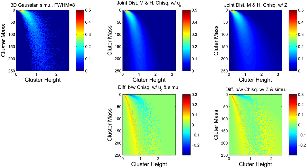
The top row of Figure 1 shows the true (simulated) joint distribution of cluster mass and peak height intensity, the Ƶ result and the 𝒰 result for 3D Gaussian noise images. The bottom row shows difference images of true and derived distributions for the Ƶ and 𝒰 results. The distributions are qualitatively similar, though for very small cluster masses and cluster height around 0.5 to 1.0, the two results tend to underestimate the truth; while for cluster mass between 0 and 50 and cluster heights between 0 and 0.5, the results can overestimate the truth. The Kullback-Leibler divergences are 1.285 for the Ƶ result and 1.610 for the 𝒰 result.

Figure 1.

Comparison of true and theoretical joint distributions of cluster mass and peak height intensity, for Gaussian images. On top left is the true distribution obtained from simulation, on the top middle is the 𝒰 result and on the top right is the Ƶ result. Below each of the theoretical results is the true minus estimated distributions. While only an intermediate result, the agreement is reasonable, with better performance obtained with the Ƶ result. All distributions are transformed by the fourth root to improve visualization. Unless otherwise noted, simulation settings used in the figures are: u_c = 2.3263 (p=0.01), 64 × 64 × 30 image at FWHM 8 voxels.

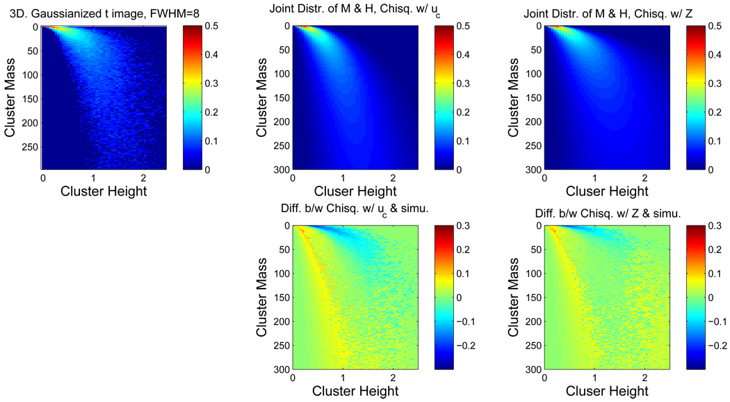
Figure 2 displays corresponding results for 3D Gaussianized t image. Again, there is little difference between the true distribution and the two results, and again the Kullback-Leibler divergence between the true distribution and the Ƶ result is smaller than that between the true distribution and the 𝒰 result (1.701 vs. 2.338). Thus, for both Gaussian images and Gaussianized images, the Ƶ result appears to be superior to the 𝒰 result.

Figure 2.

Comparison of true and theoretical joint distributions of cluster mass and peak height intensity, for Gaussianized t₁₄ images. Same format as in Figure 1. Again the agreement between simulated truth and derived theoretical result is good, with a closer match seen with the Ƶ result.

3.1.2 Accuracy of derived cluster mass null distribution

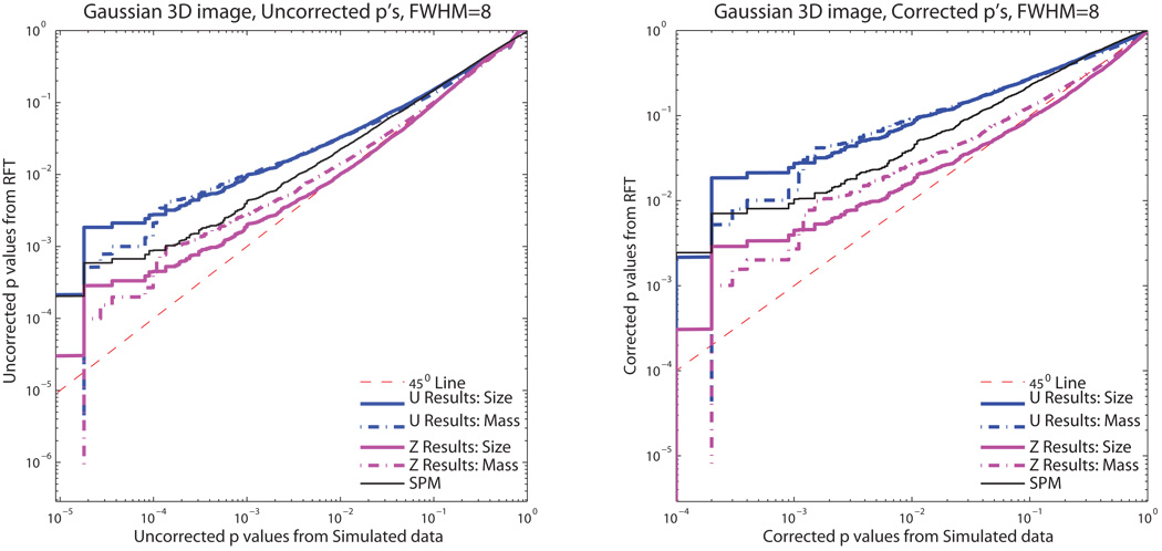
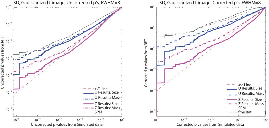
Figure 3 shows the P-P plots for 3D Gaussian null simulated data and Figure 4 3D Gaussianized t-statistic null simulated data. Both cluster mass (dot-dashed lines) and cluster size results (solid lines) are shown. For all of our derived methods, the 𝒰 results are more conservative (the null will be rejected less often than nominal) than the Ƶ results. The SPM cluster size results are also more conservative than the Ƶ results for Gaussian null simulated data and the 𝒰 results for Gaussianized t-statistic null simulated data. While our Ƶ result for cluster size exhibits some anticonservativeness, overall the Ƶ result of cluster mass is the least conservative method, while maintaining validity over most of the range of probabilities included in this simulation study.

Figure 3.

Monte Carlo simulation P-values versus theoretical P-values for uncorrected and corrected P-values with Gaussian images. Values in the plot above the identity indicate conservative performance, below the identity invalid performance. Our Ƶ cluster mass method exhibits slightly conservative performance, but much less conservative than the other methods.

Figure 4.

Monte Carlo simulation P-values versus theoretical P-values for uncorrected and corrected P-values with Gaussianized t₁₄ images. Despite Gaussianization, our Ƶ cluster mass method provides close to exact performance, and less conservative performance than other methods.

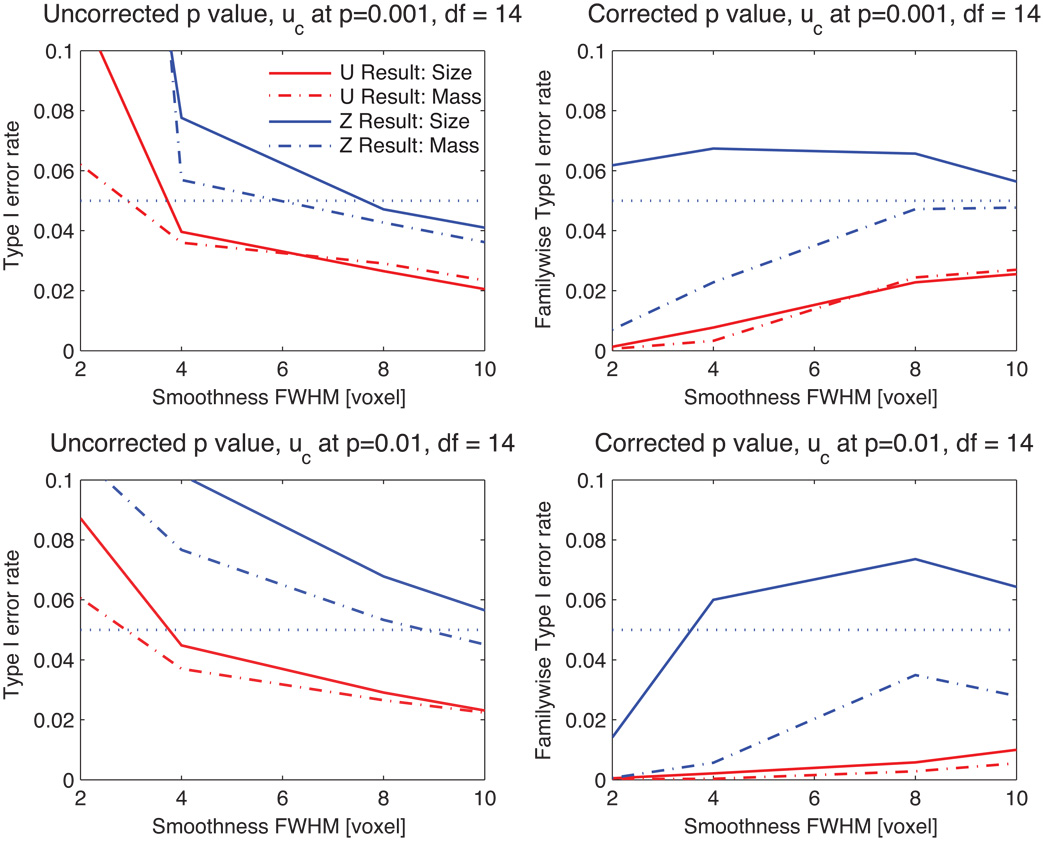
Figure 5 shows the Type I error rates for a 3D Gaussianized t image with 14 degrees of freedom with various smoothness parameters (FWHM) and cluster defining thresholds. The figure shows that the Ƶ cluster mass result provides better results for high thresholds and large FWHM than for low threshold and low FWHM. For corrected P values, this result is valid for all levels of smoothing studied, whereas the Ƶ result of cluster extent is, by and large, invalid. Furthermore, the Ƶ cluster mass corrected P-values—those that are used in practice—are always closer to the nominal significance level when correcting for multiple comparisons.

Figure 5.

Type I error rate for Gaussianized t images, for both P = 0.01 and P = 0.001 cluster-forming thresholds, with different smoothness. While uncorrected P-values perform poorly under low smoothness, our Ƶ cluster mass method has the corrected P-values are closest to the nominal α = 0.05 level without being invalid.

3.1.3 Power comparisons

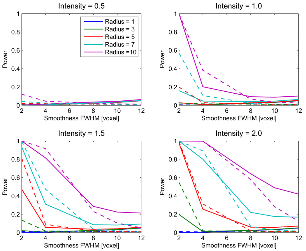
Having found our own cluster extent result to be invalid, we compare the power of our Ƶ cluster mass result only to SPM’s cluster extent result. Figure 6 illustrates simulated power for the cluster extent (SPM) and cluster mass (Ƶ). As expected, for a given intensity, the power increases with signal intensity, and, for a given radius, power increases as the signal intensity increases. When the image smoothness is low (FWHM ≤ 4 voxels), SPM cluster extent generally provides better power than the Ƶ mass result. However, for greater smoothness (FWHM ≥ 8 voxels), the Ƶ result is more powerful than SPM, regardless of signal extent or signal intensity.

Figure 6.

Power of our proposed cluster mass inference method (solid lines), compared with standard cluster extent inference method implemented in SPM (dashed lines), for different cluster sizes and signal intensities. Gaussian images were used with a cluster defining threshold of 2.3263 (p=0.01).

3.2 Real Data Evaluations

The FIAC data results show the method’s performance at high degrees-of-freedom, while the working memory data assess the method using Gaussianization of the t image.

3.2.1 FIAC data

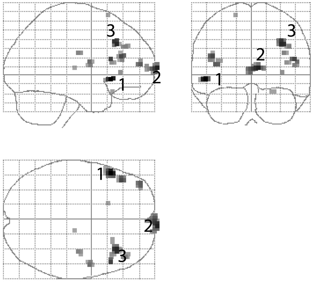
The estimated smoothness of the component fields based on the residuals is [2.4964 2.3599 1.7525] voxel FWHM with 27,862 3.0 × 3.0 × 4.0mm³ voxels. Figure 7 shows the maximum intensity projection of all clusters found with a P = 0.001 threshold, the three most prominent being a pair of bilateral activations in inferior frontal gyri and one in the frontal pole. Note that the primary auditory cortex effect did not survive P = 0.001 threshold, and inspection of the unthresholded statistic image suggests the frontal pole cluster is a false positive activation due to susceptibility artifacts. However, the general shape and size of the clusters are still representative of true positive signals and are useful for evaluating our method.

Figure 7.

Results for “sentence” effect in FIAC single subject data.

Table 1 provides the values of cluster extent, suprathreshold peak height intensity and cluster mass for each cluster, as well as the P-values, all sorted by peak height. The first three clusters have corrected significance with cluster mass, while peak height and cluster extent only find one cluster significant each. The uncorrected significances show that if a cluster is significant by any of the three methods, it is significant by cluster mass. Again, while we do not advocate use of uncorrected inferences, this demonstrates the relative sensitivity of the method.

Table 1.

Real data results for FIAC single subject data analysis, comparing extent, peak height and mass statistics for cluster inference. The cluster mass has good sensitivity, and, in particular, when any of the three inference methods are significant, cluster mass is usually significant,

Cluster No	Cluster			Uncorrected P values			Corrected P values			Location
	Extent	Height	Mass	Extent	Height	Mass	Extent	Height	Mass	(x,y,z mm)
1	13	5.09	9.35	0.0069	0.0008	0.0011	0.1606	0.0192	0.0279	(−52,22,−5)
2	24	4.52	12.54	0.0009	0.0092	0.0004	0.0238	0.2096	0.0106	(8,75,8)
3	13	4.45	7.97	0.0069	0.0122	0.0018	0.1606	0.2665	0.0451	(34,29,35)
4	5	4.10	2.09	0.0633	0.0463	0.0404	0.7999	0.6920	0.6425	(49,22,18)
5	10	4.08	3.60	0.0140	0.0508	0.0138	0.2992	0.7251	0.2959	(−44,34,21)
6	6	3.87	2.60	0.0446	0.1056	0.0269	0.6782	0.9319	0.4960	(−41,56,12)
7	5	3.65	1.22	0.0633	0.2134	0.0967	0.7999	0.9956	0.9145	(52,−2,15)
8	5	3.48	0.98	0.0633	0.3492	0.1334	0.7999	0.9999	0.9664	(73,39,32)
9	3	3.43	0.64	0.1447	0.4013	0.2324	0.9764	1.0000	0.9973	(37,−15,25)
10	1	3.34	0.25	1.0000	0.5261	0.6816	1.0000	1.0000	1.0000	(35,33,3)
11	2	3.21	0.22	0.2433	0.7304	0.7648	0.9979	1.0000	1.0000	(23,24,−19)
12	1	3.18	0.09	1.0000	0.7924	1.0000	1.0000	1.0000	1.0000	(−18,19,68)
13	1	3.16	0.07	1.0000	0.8429	1.0000	1.0000	1.0000	1.0000	(13,−19,8)

3.2.2 Working Memory Data

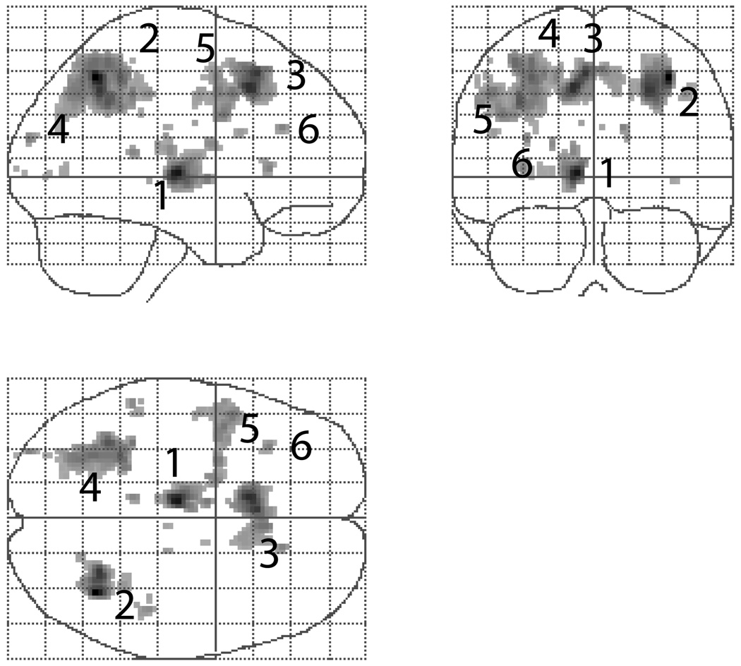
The estimated smoothness is [4.8611 6.4326 6.6156] voxel FWHM with 122,659 2.0 × 2.0 × 2.0 voxels. Figure 8 shows that all of the clusters found with a P = 0.001 cluster-forming threshold. Table 2 compares our RFT cluster mass results to an equivalent permutation method. Our RFT method finds the five largest clusters significant, as does the RFT cluster size statistic. Notable is the close correspondence between the RFT P-values and the permutation P-values.

Figure 8.

Results from item recognition effect in the working memory data.

Table 2.

Real data results for the small group fMRI data, comparing RFT parametric and permutation nonparametric inferences. Note the similarity between the RFT P-values and permutation P-values, even though the RFT method depends on many assumptions and approximations.

Cluster No	Random Field Theory Cluster Mass Inference
	Cluster			Uncorrected p-values			Corrected p-values			Location
	Extent	Height	Mass	Extent	Height	Mass	Extent	Height	Mass	(x,y,z mm)
1	347	5.47	182.19	0.0005	0.0001	0.0002	0.0043	0.0011	0.0018	(−8,−18,2)
2	540	4.99	262.29	0.0001	0.0012	0.0001	0.0007	0.0111	0.0004	(36,−58,48)
3	620	4.82	272.05	0.0000	0.0026	0.0001	0.0004	0.0231	0.0004	(−10,16,44)
4	1150	4.34	448.15	0.0000	0.0192	0.0000	0.0000	0.1602	0.0000	(−30,−46,48)
5	481	4.02	119.41	0.0001	0.0621	0.0008	0.0012	0.4313	0.0076	(−48,8,40)
6	40	3.43	5.26	0.1012	0.4110	0.1684	0.6014	0.9761	0.7836	(−34,24,4)

Cluster No‡	Permutation-based Cluster Mass Inference
	Cluster			Uncorrected P values			Corrected P values			Location
	Extent	Height	Mass	Extent	Height	Mass	Extent	Height	Mass	(x,y,z mm)
1	347	5.47	182.19	0.0018	0.0000	0.0007	0.0098	0.0002	0.0034	(−8,−18,2)
2	540	4.99	262.29	0.0008	0.0008	0.0003	0.0039	0.0051	0.0015	(36,−58,48)
3	620	4.82	272.05	0.0006	0.0018	0.0002	0.0037	0.0117	0.0012	(−10,16,44)
4	1150	4.34	448.15	0.0000	0.0132	0.0000	0.0002	0.0803	0.0002	(−30,−46,48)
5	481	4.02	119.41	0.0010	0.0461	0.0018	0.0049	0.2305	0.0093	(−48,8,40)
6	40	3.43	5.26	0.0658	0.3327	0.1202	0.2759	0.7515	0.4312	(−34,24,4)

4 Discussion

Although cluster mass inference with nonparametric permutation has been found to be a quite sensitive inference method for neuroimaging data [11], permutation is computationally intensive, not a very flexible modeling framework. Holmes provided mean of the cluster mass to the power 2/(D+2) for Gaussian random field without detailed proofs [13]. We propose a new theoretical cluster mass inference method for Gaussian images and Student’s t-statistic images, based on Gaussian RFT. Our simulation studies show that our derived null distribution is accurate, and performs well not only for Gaussian images, but also for Student’s t-statistic image. Like other RFT methods, our results depend only on the smoothness and the volume of the image. While we did not find closed form results for the P-value for an arbitrary mass value, the P-value can be quickly found based on interpolation of a pre-computed look-up table.

Our evaluations of the test’s specificity reveal that the proposed cluster mass inference method works best when the image is sufficiently smoothed, at least 4 voxel FWHM, and ideally for larger smoothness parameters (FWHM ≥ 8 voxels). We stress that this is a substantial magnitude of smoothness (typical estimated smoothness is FWHM 2–4 voxels). However, our real data evaluations found our method perform as good or better than parametric cluster size inference, even though image smoothness was only about 2 voxels FWHM in the single subject dataset. Hence, even with slightly conservative P-values, the mass statistic appears very sensitive to real data signals.

Consistent with findings using the nonparametric cluster mass inference method, our theoretical cluster mass inference statistic generally has better power than either the cluster extent inference statistic or the voxel intensity statistic, alone. This is especially true when the cluster extent and the suprathreshold peak height intensity are moderately sized. More remarkable, is that despite a large number of assumptions and a sequence of approximations, our RFT cluster mass P-values are very close to the permutation results which have very few assumptions.

The Gaussianization of t images is a shortcoming of the method, but it is not an uncommon strategy. The FSL [20] software has always (as of version 4.0) used Gaussianization of t and F images. While the SPM software has abandoned Gaussianization for voxel-wise inference ever since SPM99, its cluster extent inference has always (as of SPM5) used Gaussian and not t random field results cluster extent P-values and currently neglects the smoothness adjustment described in Appendix B.7.

Although the proposed cluster mass inference method has many good statistical properties, it has its limitations. When we derive the formulas for the marginal distribution of cluster mass, we assume that the shape of a cluster above a certain threshold is approximated by a paraboloid. This assumption is rational for a Gaussian image that has been convolved with a Gaussian smoothing kernel. However, for real data, this assumption may be too strong, even after smoothing the data. For example, we may have a large flat cluster with only one voxel of high intensity. The activated regions may also have other shapes that are not well approximated by a paraboloid. In addition, we use a Gaussian shaped correlation function to simplify the variance in the derivation. We also assume that we have stationary fields, though an extension to accommodate local variation in smoothness [12] may be possible.

While we have only attempted to derive Gaussian results, a reviewer notes that [24] derived the Hessian of a t field which, when simplified by conditioning and combined with results from [3], could provide a means to derive t cluster mass statistic.

Finally we note that, while both real data examples were fMRI, the method makes no assumptions about the modality and should operate well with PET and other types of imaging data. To this end, an extension to SPM will be available soon to allow use of our results; check the SPM Extensions website⁷ for a link.

Appendix A Cluster P values

We use nonparametric permutation to obtain uncorrected and FWE corrected cluster mass P-values on real data, to provide a comparison for our proposed parametric mass statistic. As most neuroimaging permutation literature focuses on voxel-wise inference, we briefly review nonparametric cluster inference.

An nonparametric uncorrected P-value for a single voxel is trivial, as it is just the direct application of a univariate permutation test. Defining an uncorrected P-value for clusters, however, is difficult as there is no unique way to define equivalent clusters after permutation of the data. If there are L cluster the original statistic image, in a permuted-data statistic image there will rarely be L clusters and there will almost never be a cluster in exactly the same location. Instead of matching clusters between permutations, an assumption of stationarity is made, that the distribution of cluster statistics (e.g. size, mass, local peak height, etc) does not vary with space. With such a stationarity assumption, cluster statistics can be pooled over space, and a pooled permutation distribution created. While permutation distributions typically containing K elements, where K is the number of permutations, the uncorrected cluster permutation distribution will contain ${\displaystyle {\sum }_{k=1}^K{L}_k}$ elements, where L_k is the number of clusters found in permutation k’s statistic image. The uncorrected P-value is the proportion of the ${\displaystyle {\sum }_{k=1}^K{L}_k}$ elements that are as large or larger than an observed cluster statistic.

FWE corrected cluster P-values are more straightforward, and only require creating the maximal cluster statistic distribution. Because the search over the image for the maximal statistic, no assumption of stationarity is required. Even when some regions of the image that are smoother (or, by chance, give rise to larger cluster statistics) the maximum operation naturally accounts for such variation. (Nonstationarity is a problem for parametric cluster inference, though see [12]). For each permutation the maximal cluster statistic is recorded, and the corrected P-value is the proportion of the (K) maximal elements that are as large or larger than an observed cluster statistic.

Lastly, we note that if cluster statistics are marked as significant only when FWE-significant at 0.05, there is then 95% confidence of no false positive clusters anywhere in the image. For more on FWE see [19].

B Derivation of Null Distribution of Cluster Mass

Our derivation of the distribution of cluster mass follows that of Poline et al. [23] (PWEF) with several departures. A rough outline of the derivation is as follows:

1. A second order Taylor series approximates the statistic image at a local maximum as a paraboloid, determined by peak height and curvature about the maximum.

2. The geometry of a paraboloid gives cluster extent and mass as a function of peak height and the curvature (Jacobian determinant).

3. Distribution of the curvature, conditional on peak height, is found using an assumption of a Gaussian autocorrelation function.

4. Combining two previous results relates extent and mass, conditional on peak height, to a χ² distribution. A bias correction is made using the expected Euler characteristic.

5. At this point PWEF used a small excursion assumption; we produce a pair of results, with and without this assumption.

6. Joint distribution of mass and height are found and marginalized to produce final mass result.

B.1 Notation & Preliminaries

Let Z(x) be a D-dimensional Gaussian image, with

$$\begin{array}{ccc}\hfill 𝖤(\mathbf{Z}(\mathbf{x}))& =& 0,\\ \hfill \text{Var}(\mathbf{Z}(\mathbf{x}))& =& 1,\\ \hfill \text{Var}(\mathrm{\nabla }\mathbf{Z}(\mathbf{x}))& =& \mathrm{\Lambda }\end{array}$$

for all x ∈ Ω ⊂ ℜ^D in the image volume, where ∇ is the gradient operator and Λ is the D × D matrix which parameterizes roughness. We assume the process is smooth, in that ∇² ρ(0) exists, where ρ(·) is the autocorrelation function and ∇² is the Hessian operator.

Without loss of generality, suppose there exists a local maximum at x = 0, and consider the approximating paraboloid from a second order Taylor series about x = 0

$$\mathbf{W}(\mathrm{x})=\mathbf{Z}(0)+{\mathrm{x}}^{\mathrm{T}}({\mathrm{\nabla }}^2\mathbf{Z}(0))\mathrm{x}/2$$

Suppressing the spatial index, let Z = Z(0), and denote J = | – ∇²Z(0)| the negative Jacobian determinant.

For a cluster-defining threshold u_c, let H = Z – u_c be the suprathreshold magnitude (note that we suppress the ℓ subscript used in the body of the paper). Then the geometry of the approximating paraboloid gives cluster extent as

$$S=a{2}^{D/2}{H}^{D/2}{J}^{-1/2}$$ (5)

where a = π^D/2/Γ(D/2 + 1) is the volume of the unit sphere, and mass as

$$M=2SH/(D+2).$$ (6)

B.2 Distribution of S|H

Conditional on H, PWEF showed that another Taylor series yields

$$\text{ln}J|H\approx \text{ln}|\mathrm{\Lambda }|+D\text{ln}(H+u_c)+\eta ,$$ (7)

where η is mean zero Gaussian with variance⁸

$$\text{Var}(\eta |H)=[\text{tr}(({\mathrm{\Lambda }}^{-1}\otimes {\mathrm{\Lambda }}^{-1}){\rho }^{(4)}(\mathbf{0}))-D^2]/(H+u_c).$$

While this expression is quite involved, if we assume that ρ is proportional to a Gaussian probability density function (PDF), it simplifies to Var(η|Z) = 2D/(H + u_c)². Subsequently we will need J^−1/2, and so write the exponentiated and powered equation (7) as J^−1/2 ≈ |Λ|^−1/2(H + u_c)^−D/2 exp (η/2)⁻¹. However, as in PWEF, we find that numerical evaluations of the final result are poor when η is assumed to be Gaussian (results not shown). We instead linearize the exponential,

$$J^{-1/2}|H\approx {|\mathrm{\Lambda }|}^{-1/2}{(H+u_c)}^{-D/2}{(1+\eta /2)}^{-1}$$ (8)

and approximate 1+η/2 with η′, where νη′ is ${\chi }_{\nu }^2$ variate. Matching the second moments of 1 + η/2 and η’ gives ν = 4(H + u_c)²/D. Combining with Equations (8) and Eq. (5) yields

$$S|H\approx a{2}^{D/2}{|\mathrm{\Lambda }|}^{-1/2}{(H+u_c)}^{-D/2}{H}^{D/2}{\eta \prime }^{-1}.$$ (9)

B.3 𝒰 Result for M

PWEF proceeded by using a small excursion approximation, that H is small relative to u_c, replacing H + u_c with u_c. With this change, and marginalizing out H, the expected cluster extent can be found as

$${𝖤}_{𝒰}(S)={(2\pi )}^{D/2}{|\mathrm{\Lambda }|}^{-1/2}{u}_c^{-D}.$$ (10)

However, accurate results using the expected Euler Characteristic [1] give

$${𝖤}_{\text{EC}}(S)={(2\pi )}^{D/2}{|\mathrm{\Lambda }|}^{-1/2}{u}_c^{-(D-1)}(1-\mathrm{\Phi }(u_c))/\varphi (u_c)$$ (11)

where Φ is the standard Gaussian CDF and ϕ is the standard Gaussian PDF. Hence, the approximation for S|H is scaled by

$$c_{𝒰}=\frac{{𝖤}_{\text{EC}}(S)}{{𝖤}_{𝒰}(S)}=u_c(1-\mathrm{\Phi }(u_c))/\varphi (u_c).$$ (12)

As a side note, this is Mill’s ratio [8] scaled by u_c, which will have c_𝒰 converging to 1 from below for large u_c.

The bias-adjusted result is

$$M|H\approx a{c}_{𝒰}{2}^{D/2+1}{(D+2)}^{-1}{|\mathrm{\Lambda }|}^{-1/2}{u}_c^{-D/2}{H}^{D/2+1}{\eta \prime }^{-1},$$ (13)

which is a scaled inverse χ² random variable with ${\nu }_{𝒰}=4u_c^2/D$ degrees of freedom and scale parameter

$$q_{𝒰}(H)=a{c}_{𝒰}{2}^{D/2+1}{(D+2)}^{-1}{|\mathrm{\Lambda }|}^{-1/2}{u}_c^{-D/2}{H}^{D/2+1}$$

The marginal distribution of H is approximately exponential with mean 1/u_c [1], and thus the joint PDF of M and H is

$$f_{𝒰}(M,H)\approx \frac{{(q_{𝒰}(H){\nu }_{𝒰}/2)}^{{\nu }_{𝒰}/2}}{\Gamma (\nu /2)}\frac{\text{exp}[(q_{𝒰}(H){\nu }_{𝒰}/2)/M]}{M^{{\nu }_{𝒰}/2+1}}\text{exp}[-u_{c}H]u_c$$ (14)

for M,H > 0. The uncorrected P-value for cluster mass is then found with

$$P_{𝒰}(M>m)\approx {\displaystyle {\int }_m^{\infty }{\displaystyle {\int }_0^{\infty }{f}_{𝒰}(M,H)dHdM}}$$

using numerical integration over a fine grid.

B.4 Ƶ Result for M

We repeat the preceding without the small excursion approximation. We call this the Ƶ result, since Z = H + u_c is left as is. Returning to (9) and marginalizing out H we get

$${𝖤}_{Ƶ}(S)=a{2}^{D/2}{|\mathrm{\Lambda }|}^{-1/2}𝖤\{{[H/(H+u_c)]}^{D/2}\}$$ (15)

where the final term must be found numerically for a particular u_c. This provides the bias adjustment term

$$c_{Ƶ}={𝖤}_{\text{EC}}(S)/{𝖤}_{Ƶ}(S).$$ (16)

This provides an approximation for M|H as a scaled inverse χ² random variable with ν degrees of freedom and scale parameter

$$q_{Ƶ}(H)=a{c}_{Ƶ}{2}^{D/2+1}{(D+2)}^{-1}{|\mathrm{\Lambda }|}^{-1/2}{(H+u_c)}^{-D/2}{H}^{D/2+1}$$

and joint PDF of M and H of

$$f_{Ƶ}(M,N)\approx \frac{{(q_{Ƶ}(H)\nu /2)}^{\nu /2}}{\Gamma (\nu /2)}\frac{\text{exp}[(q_{Ƶ}(H)\nu /2)/M]}{M^{\nu /2+1}}\text{exp}[-u_{c}H]u_c.$$ (17)

As before, the uncorrected P-value for cluster mass is then found with

$$P_{Ƶ}(M>m)\approx {\displaystyle {\int }_m^{\infty }{\displaystyle {\int }_0^{\infty }{f}_{Ƶ}(M,H)dHdM}}$$

using numerical integration over a fine grid.

B.5 Corrected P-values

The uncorrected P-values can be transformed into family-wise error (FWE) corrected P-values with either a Bonferroni correction for the expected number of clusters or the Poisson clumping heuristic [1,4, 10]. We opt for the later, as it provides a continuous transformation between uncorrected and corrected P-values.

A FWE corrected P-value accounts for the chance of the maximal statistic exceeding that actually observed. Assuming the clusters arise as a Poisson process, this P-value is found as

$$𝖯({\text{max}}_{\ell }{M}_{\ell }>m)\approx 1-\text{exp}\{-𝖤(L)\cdot 𝖯(M_{\ell }>m)\},$$ (18)

where 𝖤(L) is the expected number of clusters in the image. For moderate thresholds u_c the Euler characteristic will count the number of clusters, and hence we approximate 𝖤(L) ≈ 𝖤_EC(L). The most accurate results for 𝖤_EC(L) depends on the dimension and the topology of the search region [26]. For a 3D, approximately spherical search region

$${𝖤}_{\text{EC}}(L)=\mathrm{\lambda }(\mathrm{\Omega }){|\mathrm{\Lambda }|}^{1/2}{(2\pi )}^{-2}(u_c^2-1)\text{exp}[-u_c^2/2];$$ (19)

where λ(Ω) is the volume of the search region. In addition, for a high threshold u_c, the number of clusters above the threshold will be approximated by [1, 23]

$$𝖤(L)=\mathrm{\lambda }(\mathrm{\Omega }){|\mathrm{\Lambda }|}^{1/2}{(2\pi )}^{-2}{u}_c^2\text{exp}[-u_c^2/2]$$

B.6 Smoothness Estimation & Λ

The preceding results depend on the roughness of the component random fields, as parameterized by |Λ|. Worsley et al. [25] proposed re-expressing this as the FWHM Gaussian kernel required smooth an independent random field into one with roughness Λ. Assuming the smoothing is aligned with the major axes of the image, this relationship is

$${|\mathrm{\Lambda }|}^{1/2}=\frac{{(4\text{ln}2)}^{D/2}}{{\displaystyle {\prod }_d{\text{FWHM}}_d}}$$

where FWHM_d is the smoothness in the d-th dimension. If the smoothness is not known, | Λ|^1/2 can be estimated from the residual images of a general linear model [14]

B.7 Student’s t-image

Worsley et al. and Holmes [14] showed that if the roughness of the Gaussian component fields is Λ, the roughness for a Student’s t-statistic image can be approximated by Λ_T = λ_nΛ, where n > 4 is the number of scans used to generate the t image and λ_n is the correction factor [13, 25]. When applying our method to Gaussianized data we adjust Λ accordingly.

References

- 1.Adler RJ. The Geometry of Random Fields. New York: Wiley; 1981. [Google Scholar]
- 2.Bullmore ET, Suckling J, Overmeyer S, Rabe-Hesketh S, Taylor E, Brammer MJ. Global, voxel, and cluster tests, by theory and permutation, for a difference between two groups of structural MR images of the brain. IEEE Trans. Med. Imaging. 1999;18:32–42. doi: 10.1109/42.750253. [DOI] [PubMed] [Google Scholar]
- 3.Cao J. The size of the connected components of excursion sets of χ2, t, and F fields. Advances in Applied Probability. 1999;31:579–595. [Google Scholar]
- 4.Cao J, Worsley KJ. Applications of random fields in human brain mapping. In: Moore M, editor. Spatial Statistics: Methodological Aspects and Applications, Springer lecture Notes in Statistics. volume 159. Springer, New York: 2001. pp. 169–182. [Google Scholar]
- 5.Friston KJ. Testing for anatomically specified regional effects. Human Brain Mapping. 1997;5:133–136. doi: 10.1002/(sici)1097-0193(1997)5:2<133::aid-hbm7>3.0.co;2-4. [DOI] [PubMed] [Google Scholar]
- 6.Friston KJ, Frith CD, Liddle PF, Frackowiak RSJ. Comparing functional (PET) images: The assessment of significant change. J. Cereb. Blood Flow Metab. 1991;11:690–699. doi: 10.1038/jcbfm.1991.122. [DOI] [PubMed] [Google Scholar]
- 7.Friston KJ, Holmes AP, Poline J-B, Price CJ, Frith CD. Detecting activations in pet and fmri: levels of inference and power. NeuroImage. 1996;4:223–235. doi: 10.1006/nimg.1996.0074. [DOI] [PubMed] [Google Scholar]
- 8.Gordon RD. Values of mill’s ratio of area to bounding ordinate of the normal probability integral for large values of the argument. Annals of Mathematical Statistics. 1941;12:364–366. [Google Scholar]
- 9.Madic Group. Functional Imaging Analysis Contest (FIAC) 2005 http://www.madic.org/fiac/how_to_participate.html.
- 10.Hayasaka S, Nichols TE. Validating cluster size inference: Random field and permutation methods. NeuroImage. 2003;20(4):2343–2356. doi: 10.1016/j.neuroimage.2003.08.003. [DOI] [PubMed] [Google Scholar]
- 11.Hayasaka S, Nichols TE. Combining voxel intensity and cluster extent with permutaion test framework. NeuroImage. 2004;23:54–63. doi: 10.1016/j.neuroimage.2004.04.035. [DOI] [PubMed] [Google Scholar]
- 12.Hayasaka S, Phan KL, Liberzon I, Worsley KJ, Nichols TE. Nonstationary cluster-size inference with random field and permutation methods. NeuroImage. 2004;22(2):676–687. doi: 10.1016/j.neuroimage.2004.01.041. [DOI] [PubMed] [Google Scholar]
- 13.Holmes AP. Statistica Issues in functional Brain Mapping. PhD thesis. University of Glasgow; 1994. [Google Scholar]
- 14.Kiebel S, Poline JB, Friston KJ, Holmes AP, Worsley KJ. Robust smoothness estimation in statistical parametric maps using standardized residuals from the general linear model. Neuroimage. 1999;10:756–766. doi: 10.1006/nimg.1999.0508. [DOI] [PubMed] [Google Scholar]
- 15.Kullback S, Leibler RA. On information and sufficiency. Annals of Mathematical Statistics. 1951;22:79–86. [Google Scholar]
- 16.Lazar NA, Luna B, Sweeney JA, Eddy WF. Combining brains: a survey of methods for statitical pooling of information. Neuroimage. 2002;16:538–550. doi: 10.1006/nimg.2002.1107. [DOI] [PubMed] [Google Scholar]
- 17.Luo W-L, Nichols TE. Diagnosis and exploration of massively univariate fmri models. NeuroImage. 2003;19(3):1014-1–1014-32. doi: 10.1016/s1053-8119(03)00149-6. [DOI] [PubMed] [Google Scholar]
- 18.Marshuetz C, Smith EE, Jonides J, DeGutis J, Chenevert TL. Order information in working memory:fMRI evidence for partietal and prefrontal mechanism. J. Cogn. Neurosci. 2000;12(S2):130–144. doi: 10.1162/08989290051137459. [DOI] [PubMed] [Google Scholar]
- 19.Nichols TE, Hayasaka S. Controlling the familywise error rate in functional neuroimaging: A comparative review. Statistical Methods in Medical Research. 2003;12(5):419–446. doi: 10.1191/0962280203sm341ra. [DOI] [PubMed] [Google Scholar]
- 20.Analysis Group of Functional Magnetic Resonance Imaging of the Brain(FMRIB) Oxford, London, UK: Fmrib software library. http://www.fmrib.ox.ac.uk/fsl/. [Google Scholar]
- 21.Wellcome Department of Imaging Neuroscience. University of College London, London, UK: Statistical parametric mapping. http://www.fil.ion.ucl.ac.uk/spm/ [Google Scholar]
- 22.Pesarin F. Multivariate Permutation Tests. New York: Wiley; 2001. [Google Scholar]
- 23.Poline JB, Worsley KJ, Evans AC, Friston KJ. Combining spatial extent and peak intensity to test for activations in functional imaging. NeuroImage. 1997;5:83–96. doi: 10.1006/nimg.1996.0248. [DOI] [PubMed] [Google Scholar]
- 24.Worsley KJ. Local maxima and the expected Euler characteristic of excursion sets of χ2, f and t fields. Advances in Applied Probability. 1994;26:13–42. [Google Scholar]
- 25.Worsley KJ, Evans AC, Marrett S, Neelin P. Three-dimensional statistical analysis for CBF activation studies in human brain. J. Cereb. Blood Flow Metab. 1992;12:900–918. doi: 10.1038/jcbfm.1992.127. [DOI] [PubMed] [Google Scholar]
- 26.Worsley KJ, Marrett S, Neelin P, Vandal AC, Friston KJ, Evans AC. A unified statistical approach for determining significant signals in images of cerebral activation. Human Brain Mapping. 1996;4:58–73. doi: 10.1002/(SICI)1097-0193(1996)4:1<58::AID-HBM4>3.0.CO;2-O. [DOI] [PubMed] [Google Scholar]