Interaction between arthropod filiform hairs in a fluid enviroment

Abstract

Many arthropods use filiform hairs as mechanoreceptors to detect air motion. In common house crickets (Acheta domestica) the hairs cover two antenna-like appendages called cerci at the rear of the abdomen. The biomechanical stimulus-response properties of individual filiform hairs have been investigated and modeled extensively in several earlier studies. However, only a few previous studies have considered viscosity-mediated coupling between pairs of hairs, and only in particular configurations. Here we present a model capable of calculating hair-to-hair coupling in arbitrary configurations. We simulate the coupled motion of a small group of mechanosensory hairs on a cylindrical section of cercus. We have found that the coupling effects are non-negligible, and likely constrain the operational characteristics of the cercal sensory array.

1 Introduction

Many terrestrial arthropods, including crickets, cockroaches, caterpillars, spiders and scorpions, use filiform hairs as mechanoreceptors to detect the direction and magnitude of air flow. In the common house cricket (Acheta domestica) the receptor organs for this modality are two antenna-like appendages called cerci at the rear of the abdomen, see Figure 1. Each cercus is covered with approximately 1000 filiform mechanosensory hairs, ranging in length from less than 50 μm to almost 2 mm [24]. Each hair is innervated by a single spike-generating mechanosensory receptor neuron. Deflection of a hair by air currents changes the spiking activity of the associated receptor neuron at the base of the hair.

Figure 1.

A typical cercus of Acheta domestica. Total length = 1 cm.

The cercal system encodes information about the direction and dynamic properties of air currents with great accuracy and precision, and represents that information internally as a neural map [1, 13, 14, 15, 16, 17, 18, 26, 28, 29, 31, 32, 37, 38]. The interneurons that read out the information from the cercal afferent map mediate the detection, localization, discrimination and identification of signals generated by predators, mates and competitors [4, 5, 8, 9, 11, 17, 34, 36]. The cercal system is crucial for the cricket’s survival: on the basis of the information captured by this sensory system, the animal must make decisions rapidly and reliably. The cercal system has been shown to be of critical importance for a variety of behaviors including oriented escape responses [4, 5] and jumping [10]. However, it is a considerable oversimplification to class this system as an ‘escape system’, just as it would be an oversimplification to categorize our own visual system that way.

The functional characteristics of the cercal receptor array are determined by its structural features. The extremely low degree of inter-animal variability of all observable structural aspects of the cerci is remarkable. It has even been suggested (though not demonstrated conclusively) that every single filiform hair may be re-identifiable [23, 24, 44], i.e., that every adult cricket with undamaged cerci has the same number of filiform hairs, and that each hair can be catalogued with a specific relative length, position and directional movement axis differing by at most 5% across different animals. These biophysical parameters are of substantial functional importance: the mechanical filtering of stimulus information in the cercal system is determined solely by the lengths and orientations of the hairs, and by the interactions between the hairs in the array [18, 20, 27, 32, 31, 33]. The importance of the cerci for the animal’s survival, the coupling between cercal structure and function, and the extremely low inter-animal variability of cercal receptor array structure are all consistent with the conjecture that these structural attributes have been subject to selective pressure.

The main goal of this paper is to provide a computationally efficient framework to model the interaction of the cercal system with the air. This is a necessary step toward understanding the functional significance of the cercal system and the evolutionary constraints imposed by the physics of air flow at a low Reynolds number. Computational efficiency is crucial, since each cercus contains about 1000 hairs of different lengths whose movements affect the air flow and, hence, the movement of other hairs. Previous work in this area was concerned with modeling the response of a single hair to the motion of the air and only recently has the focus shifted to the analysis of the viscosity-mediated coupling between hairs [3] and characterization of a total canopy response [25].

One of the first models of single hair motion was introduced by Shimozawa and Kanou [31], which assumed periodic air flow and modeled the hair as an inverted pendulum. This work has been extended by Humphrey et al. [12], Shimozawa et al. [33] and Osborne [27]. More recently Bathellier et al. [3] studied viscosity-mediated coupling between pairs of hairs aligned with the direction of air motion on the leg of the spider Cupiennius salei. Their experimental results indicate limited interaction between these hairs, but, as the authors note, their results do not preclude significant hair interactions in other arthropods. In another recent article Magal et al. [25] attempts to characterize the response of the entire collection of hairs on the cerci of the sand cricket Gryllus bimaculatus. The response characteristic and position of each cercal hair is combined to form the canopy response. The viscosity-mediated interaction between the hairs is not taken into account.

Our work builds upon these previous investigations and continues to model the hair motion using equations describing the motion of a linear oscillator. However, our model allows the simulation of an arbitrary configuration of a group of hairs. We present a significant extension to these earlier studies by enabling the computation of the mutual interaction between hairs mediated through their interaction with the surrounding air.

In this paper we concentrate on the description of our model and numerical procedures being used, and leave the investigation of a biologically realistic model to a future paper. Section 2 contains a model of the driving air flow that stimulates the cercus. Section 3 describes the inverted pendulum model of the filiform hairs and how the hairs resist the driving air flow presented in Section 2. Section 4 contains the full system of equations that determines the motion of a population of hairs given a particular stimulus. More technical aspects of the derivation in Section 4 are located in Appendices A and B. In Section 5, we compare the performance of this model to the work of other researchers and present numerical simulations of multiple hairs. Conclusions are in Section 6.

2 Model of the air flow

We assume that the cercal system is driven by a periodic far-field air flow with amplitude U₀ and angular frequency ω. The no-slip condition at the cercal surface causes a boundary layer to form that has a smaller amplitude than the oscillatory far-field flow and is phase shifted with respect to the flow. The height of the boundary layer is on order of the lengths of the filiform hairs and thus has a non-negligible effect on hair motion. We compute the boundary layer, which we denote u_b, for axial flow along an infinite cylinder using the work of Humphrey et al. [12].

We model the total air velocity v as a sum of the boundary layer velocity u_b and a perturbation velocity u,

$$\mathbf{v}=\mathbf{u}+{\mathbf{u}}_b.$$ (1)

The velocity u is caused by the resistance of the hairs to the air motion u_b and can be thought of as a disturbance of the boundary layer due to the presence of the hairs. The perturbation velocity u is modeled by the Stokes equations, which we take as a good approximation of the Navier-Stokes equations, since the Reynolds number ranges from 10⁻⁴ to 10⁻² (see Section 2.2).

2.1 The boundary layer flow

The Navier-Stokes equations can be solved explicitly both for a periodically driven flow over an infinite plane [35] and axial flow over a bi-infinite cylinder [12]. Since each cercus is approximately a long finite cone, Shimozawa and collaborators [31, 32, 33] argued that both infinite planar and cylindrical approximations can be used successfully. This assumption is reasonable for hairs distributed in a line along the long axis of the cercus. However, we are interested in modeling groups of hairs with lateral as well as longitudinal spread. In the case of lateral spread, the curvature of the cercus effectively increases the distance between hairs and decreases viscous coupling between them. In order to capture this effect, we choose to model the cercus as a cylinder.

In this section, following Humphrey et al. [12] and Osborne [27], we solve the Navier-Stokes equations in cylindrical coordinates for axial flow over a bi-infinite cylinder, and assume that this is a reasonable approximation to the boundary layer over a finite cylinder. First allow ${\mathbf{u}}_b=[\begin{array}{lll}{u}_r\hfill & u_{\theta }\hfill & u_z\hfill \end{array}]$ to be the representation of the boundary layer in cylindrical coordinates, where the z-axis extends length-wise through the center of the cylinder. Since the far-field air flow is axial along a bi-infinite cylinder, we expect that u_b is radially symmetric and independent of the variable z at all points in space. Thus ${\mathbf{u}}_b=[\begin{array}{lll}0\hfill & 0\hfill & u_z(t,r)\hfill \end{array}]$ and the Navier-Stokes equations simplify to

$$\rho \frac{\partial u_z}{\partial t}+\frac{\partial p}{\partial z}=\mu \left[\frac{1}{r}\frac{\partial }{\partial r}\left(r\frac{\partial u_z}{\partial r}\right)\right]$$ (2)

where ρ is the density and μ is the dynamic viscosity of air, p is the fluid pressure, and t is time. The boundary conditions are u_z = 0 at the surface of the cylinder and u_z → U₀ sin ωt as r → ∞, which is the far-field flow.

Now we are able to convert (2) into a dimensionless equation using the following factors: D is the diameter of the cylinder, U₀ is the peak far-field air velocity, ω is the angular frequency of the air motion, Re is the Reynolds number, and St is analogous to the Strouhal number. We set

$$\begin{array}{llll}r=\frac{DR}{2}\hfill & p=\frac{\rho U_0^{2}P}{2}\hfill & u_z=U_{0}U\hfill & z=\frac{DZ}{2}\hfill \\ t=\frac{\tau }{\omega }\hfill & \frac{1}{Re}=\frac{2\mu }{D{U}_0\rho }\hfill & St=\frac{\omega D}{2U_0}\hfill & \hfill \end{array}$$

Then, through a substitution and a short computation (see [12, 27]) equation (2) becomes

$$\begin{array}{c}St\frac{\partial U}{\partial \tau }+\frac{1}{2}\frac{\partial P}{\partial Z}=\frac{1}{Re}\left[\frac{1}{R}\frac{\partial }{\partial R}\left(R\frac{\partial U}{\partial R}\right)\right]\\ U=0\text{at}R=1\\ U\to sin\tau \text{as}R\to \infty \end{array}$$ (3)

The solution of (3) involves a modified Bessel function of the second kind, K₀:

$$u_z=U_0{B}_c(t,r)=U_0\left(sin\omega t+\Re \left(i{e}^{i\omega t}\frac{K_0(\lambda \frac{2r}{D})}{K_0(\lambda )}\right)\right)$$ (4)

where $\lambda =\sqrt{i(Re)(St)}=\sqrt{\frac{i}{2}}\beta D,\beta =\sqrt{\frac{\omega }{2\nu }},\nu =\frac{\mu }{\rho }$ is the kinematic viscosity of air, and ${\mathbf{u}}_b=[\begin{array}{lll}0\hfill & 0\hfill & u_z\hfill \end{array}]$.

2.2 The perturbation velocity

The Reynolds number of a fluid dynamical system gives the ratio between inertial and viscous forces in that system, and is defined as

$$Re=\frac{\mid \mathbf{U}\mid d}{\nu },$$

where d is a typical length scale of the problem, |U| is the magnitude of a typical velocity of the air flow, and ν is the kinematic viscosity of the fluid. If Re ≪ 1, then the inertial forces in the system are negligible and the Navier-Stokes equations can be simplified to the Stokes equations [22]. When considering the Re of air flow around cercal hairs, we take d to be a typical hair diameter, which is approximately 5 ×10⁻⁶ m and we let ν = 1.568 × 10⁻⁵ m²/s, which is the kinematic viscosity of air at 27°C. If we limit the amplitude of the far-field flow to fall between 0.001 m/s and 0.1 m/s, which are speeds of biological relevance, then Re ranges between 3.2 × 10⁻⁴ and 3.2 × 10⁻².

Although a small Reynolds number is necessary to justify modeling fluid flow using the Stokes approximation to the Navier-Stokes equations, it is not always sufficient. In the case of oscillatory flow, there are independent time and velocity scales, which require the application of the unsteady Stokes equations. Methods needed to apply the unsteady Stokes equations to our model system have not yet been developed, so we approximate the perturbation velocity u using the Stokes equations. We can define a viscous penetration length $L_v=\sqrt{\nu /2\pi f}$ where f is the frequency of the far-field air flow. L_v is the distance over which viscosity dominates on the time scale of the driving frequency f. As long as the distance between points of interest is less than L_v then the solutions given by the steady Stokes equations are a reasonable approximation to those of the unsteady Stokes equations [30]. For larger distances, unsteady effects may be significant.

We compute the perturbation velocity u of the boundary layer u_b by solving the Stokes equations using the method of regularized Stokeslets [7]. We follow an exposition by Cortez [7] and refer the reader to the original paper for details. The 3-D Stokes flow equations take the form

$$\mathrm{\Delta }\mathbf{u}=\nabla p-\mathbf{G},\nabla ·\mathbf{u}=0$$ (5)

with applied force G(x). One special but useful example of G is that of a concentrated point force G(x) = Fδ(x−x₀) at location x₀, where F is the applied force amplitude. The flow generated by such a force is called a Stokeslet [2]. By superimposing Stokeslet velocity fields for a distribution of point forces, it is possible to find the flow generated by the forcing of more complicated structures, e.g. one dimensional filaments. However, Stokeslet velocity fields are singular at points where concentrated forces are applied. Cortez [7] developed a method to avoid this singularity by applying a force in a δ-neighborhood of a singularity by using a radially symmetric blob function φ_δ. Then equations (5) take the form

$$\mathrm{\Delta }\mathbf{u}=\nabla p-\mathbf{F}{\phi }_{\delta },\nabla ·\mathbf{u}=0$$ (6)

where F is a constant vector (for derivations of the forces F that we use in equations (6), see Sections 2.3, 3.2, and 3.3). The blob function that we use to calculate the regularized Stokeslets in our model is

$${\phi }_{\delta }(r)=\frac{15{\delta }^4}{8\pi {(r^2+{\delta }^2)}^{7/2}}$$

from [6]. To solve equations (6), we take the divergence of the first equation and use the second equation to obtain

$$\mathrm{\Delta }p=\nabla ·\mathbf{F}{\phi }_{\delta }=[{\phi }_{\delta }(\nabla ·\mathbf{F})+\nabla {\phi }_{\delta }·\mathbf{F}]=\nabla {\phi }_{\delta }·\mathbf{F},$$

where the last equality follows from the fact that F is a vector of constants implying ∇ · F = 0. Let G_δ be the solution to ΔG_δ = φ_δ. Then through an easy calculation we have that

$$p=\nabla G_{\delta }·\mathbf{F}$$

Now put p back into the first equation in (6) to obtain

$$\mathrm{\Delta }\mathbf{u}=[(\mathbf{F}·\nabla )\nabla G_{\delta }-\mathbf{F}{\phi }_{\delta }].$$

Let B_δ be the solution to ΔB_δ = G_δ. A straightforward calculation yields the solution

$$\mathbf{u}=[(\mathbf{F}·\nabla )\nabla B_{\delta }-\mathbf{F}{G}_{\delta }].$$

Notice that this equation is linear in applied force F. The linearity allows us to compute the velocity at any point x resulting from a force applied at any point y, where the points x and y may coincide. If we fix a discretized set of points at which we compute the velocity, and a set of points where we apply the force, then we can represent the linear solution map by a matrix M

$$\mathbf{u}=M\mathbf{F}.$$

In the cercal model, we represent the velocity induced at the i-th hair by forces at the j-th hair by the following notation

$${\mathbf{u}}^{(i)}=M^{(i,j)}{\mathbf{F}}^{(j)},$$ (7)

where u⁽ⁱ⁾ and F^(j) represent concatenations of three dimensional vectors, since the cercal hairs are discretized (see Section 3.1). This concept of concatenating vectors, one row vector for each point on a hair, is used heavily in this paper. We will attempt to distinguish between 3-vectors and concatenations of vectors whenever the notation is ambiguous.

If the matrix M is invertible and we have a predetermined set of velocities at some collection of points, then we can compute the forces at another (possibly identical) set of points that produce those velocities. We denote the calculation of such an inverse problem by

$$\mathbf{F}:=M^{-1}\mathbf{u}.$$ (8)

2.3 Boundary conditions

The boundary layer u_b is zero at the surface of the cercus, but the perturbation velocity u can cause nonzero velocities at the surface. We enforce the no-slip condition on the cercus by imposing a discretization scheme and using the inverse computation for regularized Stokeslets (8) derived in the last section.

We discretize a portion of the cylinder representing the cercal surface and let be the collection of all discretization points p on the cylinder. At each point p we wish to impose a force ${\mathbf{F}}_{bc}^{(p)}$ that will cause the velocity of the air to be zero at each point p ∈ . We denote the collection of boundary forces ${\mathbf{F}}_{bc}^{(p)}$ by ${\mathbf{F}}_{bc}^{(\mathcal{P})}$ and we denote a perturbation velocity at a point p by u^(p). Let u⁽⁾:= (u^(p₁), u^(p₂),…, u^(pn)) be a concatenation of the perturbation velocities at all points p_i ∈ . We want the total resulting velocity on the cercus to be zero, so we want to know what forces ${\mathbf{F}}_{bc}^{(\mathcal{P})}$ will induce velocities of −u⁽⁾. Thus we solve

$${\mathbf{F}}_{bc}^{(\mathcal{P})}:={(M^{(\mathcal{P},\mathcal{P})})}^{-1}(-{\mathbf{u}}^{(\mathcal{P})})=-{(M^{(\mathcal{P},\mathcal{P})})}^{-1}{\mathbf{u}}^{(\mathcal{P})}.$$ (9)

The forces ${\mathbf{F}}_{bc}^{(\mathcal{P})}$ calculated in this manner are then used to compute a further perturbation of the boundary layer.

3 Model of the hair

Each filiform hair is supported at its base by a viscoelastic socket membrane that enables the hair to pivot within its socket, rather than bending along its shaft [40, 42, 41, 43, 39]. Therefore, we model each hair as a rigid rod that swings in its socket as a linear, inverted pendulum [12, 31, 32, 20, 21, 27]. The trajectory of each hair is described by the angle θ(t) that the hair makes with its resting position as it moves in response to the driving flow. The primary determinants of each hair’s response properties, and hence its motion θ(t), are its length, mass and the viscoelastic properties of its socket. These properties in turn determine the linear oscillator parameters of the hair: the moment of inertia I, the spring stiffness S and the torsional resistance coefficient R. In addition, each hair has a preferred plane of motion determined by the properties of its cuticular socket and defined by a unit normal n. The four parameters I, R, S, and n modulate how each hair resists the flow through the effects of two forces: F_con is the force that constrains the hair to move rigidly in a plane and F_IRS is the force that dynamically resists the flow within the plane of motion. In this section, we describe the calculation of these forces, which are used in the computation of the perturbation velocity u, equations (6).

3.1 Parameter Selection

The population of hairs is indexed by i = 1,…, N and each hair is discretized into n_i equidistant points, denoted by ${\mathbf{x}}_j^{(i)}$, j = 1, …, n_i. The distance between the neighboring points is s,

$$\mid {\mathbf{x}}_j^{(i)}-{\mathbf{x}}_{j-1}^{(i)}\mid =s.$$

These points can be thought of as vectors that start at the base of the i-th hair and end at ${\mathbf{x}}_j^{(i)}$. We will denote $r_j^{(i)}=\mid {\mathbf{x}}_j^{(i)}\mid =js$ to be the length of this vector.

The length of a hair, L⁽ⁱ⁾, determines the values of several other hair parameters through allometric relationships. Shimozawa et al. [33] performed regression analyses on hair length and the torsional resistance constant R⁽ⁱ⁾ and restoring constant S⁽ⁱ⁾. According to their work,

$$S^{(i)}\approx 1.90\times {10}^{-11}{(L^{(i)}\times {10}^3)}^{1.67}$$ (10)

$$R^{(i)}\approx 2.88\times {10}^{-14}{(L^{(i)}\times {10}^3)}^{2.77},$$ (11)

where L⁽ⁱ⁾ is the length of the i-th hair in meters. The inertial parameter I⁽ⁱ⁾ is also related to hair length via mass, which is calculated using the shape and basal thickness of a hair. Kumagai et al. [21] found the following relationship between the base diameter $d_0^{(i)}$ of a hair and its length:

$$d_0^{(i)}\approx 8.34\times {10}^{-4}{(L^{(i)})}^{0.67},$$ (12)

where L⁽ⁱ⁾ is again in meters. In the same paper, Kumagai et al. [21] describe the shape of the hair as a paraboloid with a diameter d⁽ⁱ⁾(l) that is determined at each height l along hair i by the formula

$$d^{(i)}(l)=d_0^{(i)}{\left(1-\frac{l}{L^{(i)}}\right)}^{0.52},$$ (13)

where $d_0^{(i)}$ is the base radius of hair i and L⁽ⁱ⁾ is the length of hair i.

Each point ${\mathbf{x}}_j^{(i)}$ on the i-th hair is associated with a mass $m_j^{(i)}$. We assign an approximate value to the mass $m_j^{(i)}$ by combining (13) with the density of the cuticle, ρ_c = 1.1 × 10³ kg m⁻³. We suppose that each point on the hair is centered in a cylinder with radius determined by equation (13) and height s, where s is the distance between points on a hair. So the mass of point ${\mathbf{x}}_j^{(i)}$ is given by

$$m_j^{(i)}=\pi {\left(\frac{d_j^{(i)}}{2}\right)}^{2}s{\rho }_c$$

where $d_j^{(i)}/2$ is radius of the i-th hair at a distance $r_j^{(i)}$ from the base of the hair. Then the inertial parameter I⁽ⁱ⁾ can be calculated as follows:

$$I^{(i)}=\sum _{j=1}^{n_i}{m}_j^{(i)}{(r_j^{(i)})}^2.$$ (14)

As mentioned earlier, each hair has a preferred plane of motion. For ease of computation, we make the stricter assumption that each hair is constrained to move only in its preferred plane. We characterize this plane by a unit normal n⁽ⁱ⁾. The orientation of n⁽ⁱ⁾ is selected in such a way that ${\mathbf{n}}^{(i)}\times {\mathbf{x}}_j^{(i)}$ gives the positive direction of the motion of the hair, defined as having a positive z-coordinate. The motion of the hair will be described by the angle θ(t) with the positive x axis, see Figure 2. More generally, the rest position of a hair need not be vertical, but for now we consider only this simplified case.

Figure 2.

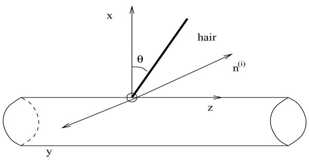
The coordinate system is centered at the root of the hair. In this example, the vector n⁽ⁱ⁾ points in the direction of the negative y axis and thus the hair moves in the (x, z)-plane. The angle θ is the angle of the hair with the positive x-axis.

3.2 Dynamic resistive forces

As in previous studies [3, 12, 25, 33], we assume that the i-th cricket hair resists the motion of the air with a torque of

$$\tau =-I^{(i)}{\ddot{\theta }}^{(i)}(t)-R^{(i)}{\stackrel{.}{\theta }}^{(i)}(t)-S^{(i)}{\theta }^{(i)}(t)$$ (15)

where I⁽ⁱ⁾ is the moment of inertia, R⁽ⁱ⁾ is the torsional resistance coefficient, S⁽ⁱ⁾ is the spring constant, and θ⁽ⁱ⁾(t) is the angular position of the i-th hair. In this section, we consider only a single hair, so we will drop the superscript indicating the identity of the hair. We want to convert the above torque into force. However, since τ = F×x, we can only recover the magnitude of the force that acts perpendicular to the hair from (15). We recover the direction of the force when we take into account the centripetal force necessary for the hair to remain attached to the surface of the cercus.

It is most convenient to consider each of the three terms on the right hand side of (15) separately. We can write τ = I(α_I + α_R + α_S), where each a_* is the angular acceleration corresponding to −Iθ̈(t), −Rθ̇ (t), or −Sθ(t). Let F_I,j, F_R,j, and F_S,j represent the amplitude of the inertial force, of the torsional resistance force, and of the restoring force at point j of a hair respectively. Then we have that the corresponding total torques along the hair are

$$\sum _{j=1}^n{F}_{I,j}{r}_j=I{\alpha }_I=-I\ddot{\theta }(t)$$ (16)

$$\sum _{j=1}^n{F}_{R,j}{r}_j=I{\alpha }_R=-R\stackrel{.}{\theta }(t)$$ (17)

$$\sum _{j=1}^n{F}_{S,j}{r}_j=I{\alpha }_S=-S\theta (t),$$ (18)

where r_j is the distance from the base of the hair to point x_j. Using these formulae, we can solve for each of α_* and hence for F_*,j, where * = I, R, S.

First consider the inertial forces F_I,j. By equation (16), α_I = −θ̈(t), and hence the force at the j-th point, F_I,j, must be mass times linear acceleration or

$$F_{I,j}=m_j{r}_j{\alpha }_I=-m_j{r}_j\ddot{\theta }(t).$$

Now consider F_R,j, the magnitude of the torsional resistance forces along the hair. From equation (17), we see that α_R = (−R/I)θ̇(t). Thus we obtain

$$F_{R,j}=m_j{r}_j{\alpha }_R=-R\stackrel{.}{\theta }(t)\frac{m_j{r}_j}{I}.$$

An analogous argument using equation (18) leads to the formula for the amplitude of the restoring force

$$F_{S,j}:=-S\theta (t)\frac{m_j{r}_j}{I}.$$

So the amplitude of the total force with which a point x_j resists the moving air is

$$F_{p,j}=F_{I,j}+F_{R,j}+F_{S,j}=-m_j{r}_j\ddot{\theta }(t)-R\stackrel{.}{\theta }(t)\frac{m_j{r}_j}{I}-S\theta (t)\frac{m_j{r}_j}{I}.$$

Here the subscript p stands for ‘perpendicular’ since direction of this force is perpendicular to the shaft of the hair and in the direction that opposes the motion of the hair. If r is a unit vector representing the position of the hair, then this direction can be expressed as h:= n×r (see Figure 3). Therefore F_p,j = F_p,jh.

Figure 3.

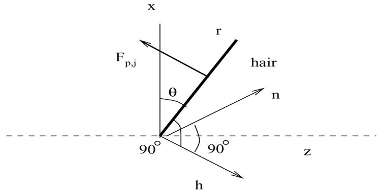
The direction h and the computation of the direction of the force F_p,j.

To compute the centripetal force, consider an element at location r_j along the hair. Since the hair is attached to the cercus, the j-th point on the hair moves along an arc of a circle of radius r_j with position (r_j cos(θ(t)), r_j sin(θ(t))) in the hair’s plane of motion. The acceleration of the j-th point is therefore

$$r_j\ddot{\theta }(-sin(\theta ),cos(\theta ))-r_j{\stackrel{.}{\theta }}^2(cos(\theta ),sin(\theta )).$$

The second term is the centripetal acceleration, therefore the centripetal force acting on the j-th point is

$${\mathbf{F}}_{\mathit{cent},j}:=-m_j{r}_j\mid \stackrel{.}{\theta }{\mid }^2\mathbf{r},$$

where r is a unit vector along the hair, r = (cos(θ), sin(θ)). The force F_cent,j does not contribute to the torque τ, since it points along the hair, but it does determine the final direction of the force at each point on the hair, and therefore affects viscosity-mediated coupling between hairs.

The total force F_IRS,j at the j-th point on the hair is the sum

$$\begin{array}{l}{\mathbf{F}}_{\mathit{IRS},j}={\mathbf{F}}_{I,j}+{\mathbf{F}}_{S,j}+{\mathbf{F}}_{R,j}+{\mathbf{F}}_{\mathit{cent},j}\\ =-m_j{r}_j\left[\left(\ddot{\theta }(t)+\frac{R\stackrel{.}{\theta }(t)}{I}+\frac{S\theta (t)}{I}\right)\mathbf{h}+\mid \stackrel{.}{\theta }{\mid }^2\mathbf{r}\right]\end{array}$$ (19)

In the text we will occasionally refer to F_IRS for an entire hair. F_IRS is the concatenation of F_IRS,j over all points j of the hair.

3.3 Constraining forces

Each hair is modeled as a collection of points that are constrained to move as a rigid rod within a particular plane of motion. So the j-th point of hair i moves at a linear speed of ${\stackrel{.}{\theta }}^{(i)}{r}_j^{(i)}{\mathbf{h}}^{(i)}$, where r and h are defined in Sections 3.1 and 3.2 respectively. To ensure that the effect of this collection of points on the surrounding fluid mimics that of a rigid rod, we must implement a no-slip condition about hair i. First we find the difference between the linear velocity of the point and the perturbed boundary layer at that same point. This difference is ${\mathbf{v}}_j^{(i)}-{\stackrel{.}{\theta }}^{(i)}{r}_j^{(i)}{\mathbf{h}}^{(i)}$, where ${\mathbf{v}}_j^{(i)}={\mathbf{u}}_j^{(i)}+{\mathbf{u}}_{b,j}^{(i)}$ from equation (1). Then we calculate the collection of forces ${\mathbf{F}}_{\mathit{con}}^{(i)}$ along the i-th hair required to negate all the velocities ${\mathbf{v}}_j^{(i)}-{\stackrel{.}{\theta }}^{(i)}{r}_j^{(i)}{\mathbf{h}}^{(i)}$. For ease of notation, allow ${\mathbf{r}}_h^{(i)}$ and v⁽ⁱ⁾ to be the concatenations of $r_j^{(i)}{\mathbf{h}}^{(i)}$ and ${\mathbf{v}}_j^{(i)}$ along hair i respectively. Then using expression (8), we can write

$${\mathbf{F}}_{\mathit{con}}^{(i)}:=-{(M^{(i,i)})}^{-1}({\mathbf{v}}^{(i)}-{\stackrel{.}{\theta }}^{(i)}{\mathbf{r}}_h^{(i)}),$$ (20)

where we follow the notation convention mentioned in the discussion of regularized Stokeslets (7).

The constraining forces acting along the i-th hair, ${\mathbf{F}}_{\mathit{con}}^{(i)}$, can have an effect on other hairs through viscosity-mediated coupling. As an example, consider the extreme case when the plane of motion of the hair is perpendicular to the direction of the ambient flow. In this case the hair does not move since no component of the driving air lies in the plane of motion of the hair. All resistive forces (Section 3.2) will be zero, since they are derived from θ, θ̇, and θ̈, which are zero when the hair is stationary. If we do not take into account the forces ${\mathbf{F}}_{\mathit{con}}^{(i)}$, then this stationary hair would have no effect on other hairs. This contradicts the observation that since the hair is a solid obstacle to the flow, its presence must affect the motion of other hairs in close proximity.

The forces ${\mathbf{F}}_{\mathit{con}}^{(i)}$ are summed with the previously calculated forces ${\mathbf{F}}_{\mathit{IRS}}^{(i)}$ and ${\mathbf{F}}_{bc}^{(\mathcal{P})}$ to calculate the perturbation velocity u via equations (5).

$$\mu \mathrm{\Delta }{\mathbf{u}}^{(i)}=\nabla p^{(i)}-(\sum _{j=1}^N{\mathbf{F}}_{\mathit{IRS}}^{(j)}+\sum _{\begin{array}{l}j=1\\ j\ne i\end{array}}^N{\mathbf{F}}_{\mathit{con}}^{(j)}+{\mathbf{F}}_{bc}^{(\mathcal{P})})$$ (21)

$$\nabla ·{\mathbf{u}}^{(i)}=0.$$ (22)

4 Equations of Motion

Now that we have calculated the perturbed velocity field, v = u_b + u, we can derive the system of differential equations that governs the hair motion, θ (t), from the relationship between angular velocity and angular momentum.

4.1 Angular velocity

In this section we compute the angular velocity θ̇ ⁽ⁱ⁾ of the i-th hair, i = 1, …, N from the total air velocity v⁽ⁱ⁾ along the hair. The angular momentum Ω⁽ⁱ⁾ imparted to the i-th hair from the moving air is the cross product of position and momentum summed over all of the points along the hair,

$${\mathbf{\Omega }}^{(i)}=\sum _{j=1}^n{\mathbf{x}}_j^{(i)}\times \left(m_j{\mathbf{v}}_j^{(i)}\right)$$

where ${\mathbf{v}}_j^{(i)}$ is the velocity of the air at the point ${\mathbf{x}}_j^{(i)}$. In the remaining part of this section we consider only a single hair, so we drop the superscript indicating the identity of the hair.

Since we constrain the hair to planar motion perpendicular to unit vector n, the vector Ω points along n and we obtain

$$\mathbf{\Omega }=\left[\sum _{j=1}^n({\mathbf{x}}_j\times (m_j{\mathbf{v}}_j))·\mathbf{n}\right]\mathbf{n}.$$

We assume that the hair is completely rigid. Therefore the angular momentum Ω imparted by the flow has magnitude

$$\mid \mathbf{\Omega }\mid =I\mid \stackrel{.}{\theta }\mid ,$$

where I is the moment of inertia of the discretized hair (see equation (14)). Thus, we have that

$$\begin{array}{l}\mid \stackrel{.}{\theta }\mid =\frac{\mid \mathbf{\Omega }\mid }{I}=\frac{\mid {\sum }_{j=1}^n{\mathbf{x}}_j\times (m_j{\mathbf{v}}_j)·\mathbf{n}\mid }{I}\\ \Rightarrow \stackrel{.}{\theta }=\frac{{\sum }_{j=1}^n({\mathbf{x}}_j\times (m_j{\mathbf{v}}_j))·\mathbf{n}}{I}\end{array}$$ (23)

4.2 The system of differential equations

The equations (4), (9), (19), (20), (21), (22), and (23) describe the model cercal system, and are listed below for reference. We rescale these equations (see Appendix A) before solving them.

$$\begin{array}{l}{\mathbf{u}}_b=U_0{B}_c(t,\mathit{x})\\ \mu \mathrm{\Delta }{\mathbf{u}}^{(i)}=\nabla p^{(i)}-(\sum _{j=1}^N{\mathbf{F}}_{\mathit{IRS}}^{(j)}+\sum _{\begin{array}{l}j=1\\ j\ne i\end{array}}^N{\mathbf{F}}_{\mathit{con}}^{(j)}+{\mathbf{F}}_{bc}^{(\mathcal{P})}){\phi }_{\delta }\\ \nabla ·{\mathbf{u}}^{(i)}=0\\ {\mathbf{F}}_{\mathit{IRS},j}^{(i)}=-m_j^{(i)}{r}_j^{(i)}\left[\left({\ddot{\theta }}^{(i)}(t)+\frac{R^{(i)}{\stackrel{.}{\theta }}^{(i)}(t)}{I^{(i)}}+\frac{S^{(i)}{\theta }^{(i)}(t)}{I^{(i)}}\right){\mathbf{h}}^{(i)}+\mid {\stackrel{.}{\theta }}^{(i)}(t){\mid }^2{\mathbf{r}}^{(i)}\right]\\ {\mathbf{F}}_{\mathit{con}}^{(i)}=-{(M^{(i,i)})}^{-1}({\mathbf{v}}^{(i)}-{\stackrel{.}{\theta }}^{(i)}{\mathbf{r}}_h^{(i)})\\ {\mathbf{F}}_{bc}^{(\mathcal{P})}=-{(M^{(\mathcal{P},\mathcal{P})})}^{-1}({\mathbf{u}}^{(\mathcal{P})})\\ {\stackrel{.}{\theta }}^{(i)}=\frac{{\sum }_{k=1}^{n_i}({\mathbf{x}}_k^{(i)}\times m_k^{(i)}{\mathbf{v}}_k^{(i)})·{\mathbf{n}}^{(i)}}{I^{(i)}}\end{array}$$ (24)

The core of our computation is the last equation above, equation (24), because we wish to solve for the angular position of each hair as a function of time. However, an explicit method of solution based on a straightforward numerical differentiation $\ddot{\theta }=\frac{d}{d\theta }\stackrel{.}{\theta }$ exhibits instability. This occurs because the right hand side of (24) depends on the perturbation velocity u, which in turn depends on the force ${\mathbf{F}}_{\mathit{IRS}}^{(i)}$. Since ${\mathbf{F}}_{\mathit{IRS}}^{(i)}$ is calculated from θ̈ ^(j) and θ̇ ^(j) for j = 1, …, N, we seek to rewrite equation (24) with θ̈ ^(j) j = 1, …, N on the left hand side and θ̇ ^(j) j = 1, …, N on the right hand side.

At every position the velocity v has four components, three of which make up the perturbation velocity:

$$\mathbf{v}=\mathbf{u}+{\mathbf{u}}_b={\mathbf{u}}_{\mathit{IRS}}+{\mathbf{u}}_{\mathit{con}}+{\mathbf{u}}_{bc}+{\mathbf{u}}_b,$$ (25)

where u_IRS is the velocity induced by all dynamic resistive forces, ${\mathbf{F}}_{\mathit{IRS}}^{(i)}$, on all hairs; u_con is the velocity induced by all forces that ensure a no-slip condition about a rigid hair, ${\mathbf{F}}_{\mathit{con}}^{(i)}$; u_bc is the velocity caused by all forces that ensure a no-slip boundary condition on the cercus, ${\mathbf{F}}_{bc}^{(\mathcal{P})}$; and u_b is the boundary layer or driving velocity. Our goal is to explicitly compute θ̈ ^(j) for j = 1, …, N in the expression of the velocity v on the right hand side of (24). Note that u_IRS depends directly on θ̈ ^(j) since u_IRS is a function of ${\mathbf{F}}_{\mathit{IRS}}^{(j)}$, which depends on θ̈ ^(j) (see (19)). Since u_bc and u_con depend on v these velocities depend on θ̈ ^(j) as well. Furthermore, through this dependence on v, the computation of u_bc depends on u_con and vice-versa. In order to be able to solve for θ̈ ^(j) explicitly, we make an assumption that, in a given time step, F_bc and F_con are computed only from u_IRS + u_b, rather than from v given by equation (25). With this assumption the fifth and sixth equations above (equations (20) and (9)) take the form

$${\mathbf{F}}_{\mathit{con}}^{(i)}=-{(M^{(i,i)})}^{-1}({\mathbf{u}}_{\mathit{IRS}}^{(i)}+{\mathbf{u}}_b^{(i)}-{\stackrel{.}{\theta }}^{(i)}{\mathbf{r}}_h^{(i)}),{\mathbf{F}}_{bc}^{(\mathcal{P})}=-{(M^{(\mathcal{P},\mathcal{P})})}^{-1}({\mathbf{u}}_{\mathit{IRS}}^{(\mathcal{P})}),$$

where ${\mathbf{u}}_{\mathit{IRS}}^{(i)}$ and ${\mathbf{u}}_b^{(i)}$ are to be taken as concatenations of velocity vectors along hair i and ${\mathbf{u}}_b^{(\mathcal{P})}$ is dropped from the second equation since u_b = 0 at all points in . Since u_bc and u_con are calculated directly from F_bc and F_con respectively, they too depend only on u_IRS + u_b. This imposes an ordering within a time step, where u_IRS and u_b are calculated first, then u_bc and u_con are calculated simultaneously from u_IRS + u_b. The effects of the neglected velocities in the computations will be transmitted indirectly by numerically integrating the above system of equations.

After some algebra (see Appendix B for the derivation), we find a linear relationship equivalent to the above system of equations:

$$A\ddot{\mathit{\theta }}=\mathbf{b},$$

where θ̈ is a vector containing the angular acceleration for each hair, A is a mass matrix that depends on (t, θ) and b is a vector that depends on (t, θ, θ̇). By adding the trivial equations $\frac{d}{dt}{\theta }^{(i)}={\stackrel{.}{\theta }}^{(i)}$ we have a system of 2N first order differential equations in unknown variables θ̇ ⁽ⁱ⁾ and θ ⁽ⁱ⁾ for i = 1, …, N. This system is well behaved numerically and we solve it using the stiff ODE solver ode15s in Matlab to advance the hair motion.

5 Results

5.1 Comparisons to previous work

To validate our model, we compared our numerical simulations to the work of other researchers. We first tested our model by simulating the motion of a single hair using the parameter set given in Humphrey et al. [12], Figure 12a, b. The purpose of Figure 12 in [12] is to demonstrate the remarkable sensitivity of the hair response on the torsional damping and restoring constants (R and S) exhibited by the motion of the filiform hair. Three different R and S pairs are applied to an identical hair and the resultant maximum deflection and angular velocity are plotted versus frequency. Our results are pictured in Figure 4 for the same set of parameters: hair length = 500 μm; hair diameter = 7 μm; cercus diameter = 2 mm; and magnitude of far-field air flow = 5 mm/s. Following the line styles in Figure 12 of Humphrey et al. [12], the solid lines labeled A in Figure 4 correspond to R and S values of 1×10⁻¹⁵ N ms/rad and 4×10⁻¹² N m/rad respectively, the dashed lines labeled B correspond to R = 0 and S = 4 × 10⁻¹² N m/rad, and the dotted lines labeled C correspond to R = 0 and S = 3 × 10⁻¹² N m/rad. The discretization scheme for the cylindrical section used to model the cercus (see Section 2.3) is described in the figure caption. Larger portions of a cylindrical cercus add computation time without affecting results more than a few percent (results not shown) and also may add unnecessary error given the assumptions of our model (see Sections 2.2 and 5.2).

Figure 4.

Comparison to Figure 12 of Humphrey et al. [12]: hair length = 500 μm; cercus diameter = 2 mm; and magnitude of driving flow = 5 mm/s. A (solid line): R = 1 ×10⁻¹⁵ N ms/rad, S = 4 ×10⁻¹² N m/rad, hair diameter = 7 μm; B (dashed line): R = 0, S = 4 × 10⁻¹² N m/rad, hair diameter = 7 μm; C (dotted line): R = 0, S = 3 × 10⁻¹² N m/rad, hair diameter = 7 μm; D (dot-dash line): R ≈ 4.2 × 10⁻¹⁵ N ms/rad, S ≈ 6.0 × 10⁻¹² N m/rad, hair diameter ≈ 5 μm. The cercus is modeled as a 200μm long length of cercus with π/4 radians on either side. The discretization scheme consists of 15 μm spacing between hair points and 28 μm spacing between cercal points. A. Maximum excursion in degrees as a function of frequency. B. Maximum velocity in radians/second as a function of frequency.

Our results are qualitatively similar to those of Humphrey et al. [12]. The relative positions of the lines representing the displacement and velocity of the hair with different R and S pairs are identical to those in Figure 12 of Humphrey et al. [12], and the shapes of the curves are similar, although the slopes in Figure 4 are less steep and the location of the peaks in the graphs disagree by as much as 25 Hz. The largest differences in amplitude between Figure 4. A and Figure 12a do not exceed 13% and these differences are most evident below 100 Hz. Likewise, the largest differences in amplitude between the curves in Figure 4. B and Figure 12b are between 10 and 20% at 50 Hz, with the differences rapidly falling off to well below 5%, allowing for the peak shift. Given that our model relies on a discretization of the cercal system and the model of Humphrey et al. [12] does not, we believe that Figure 4 is a reasonable match to the results presented in Figure 12 of that paper. Additionally, most of the differences are seen in the lower half of the frequency values examined, which may be partly explained by the fact that the theoretical analysis in Humphrey et al. [12] applies to frequencies greater than 80 Hz and the results of our model are most accurate at lower frequencies (see Section 5.2).

Like Humphrey et al. [12], we see a strong dependence on the parameters R and S in determining the motion of a filiform hair. Therefore, we use the experimentally determined values of R and S from Shimozawa et al. [33], which are allometrically related to hair length (see equations (10) and (11)). We also use an allometric relationship between hair length and base diameter [21] (see equation (12)). This work from Shimozawa et al. [33] and Kumagai et al. [21] indicates that, on average, a 500 μm hair will have a diameter of 5 μm, an R value of 4.2 × 10⁻¹⁵, and an S value of 6.0 × 10⁻¹². Using these changed parameters, our model predicts that a 500 μm hair on a 2 mm cercus driven by a 5 mm/s oscillating flow exhibits maximum displacement and velocity as seen in Figure 4, line D. Under these values of R and S, the maximum displacement and velocity curves are greatly depressed; the maximum displacement is about 60% of line A in the left half of Figure 4. A, and the maximum velocity is about 50% of line A when it peaks in Figure 4. B.

We also compared our model to data collected by Kumagai et al. [20], who studied the mobility of cricket filiform hairs ranging in length from 160 to 1484 μm. Shimozawa et al. [33] used this data to dynamically fit the pendulum parameters of the hair, I, R, and S, and then reconstructed the movement of the hairs in Figure 6 of their paper. Figure 5 below compares to Figure 6. D in Shimozawa et al. [33]. For this figure, we used the longest set of hairs observed by Kumagai et al. [20]. We assigned basal hair diameter using equation (12) and calculated the hair inertia I from equation (14). We estimated R and S values for each hair from Figures 4 and 5 of Shimozawa et al. [33]. Since the cercal diameter was not provided, we assigned the diameter to be 500 μm based on the work of Osborne [27]. In the discretization scheme, we allowed a 200 μm long section of cercus with π/4 radians to either side, 10 μm spacing between hair points, and 28 μm spacing between cercal points.

Figure 5.

Comparison to data and reconstruction in Shimozawa et al. [33]. Hair lengths indicated in legend; hair basal diameters estimated by equation (12); R and S parameters estimated from Figures 4 and 5 of Shimozawa et al. [33]; cercal diameter 500μm; discretization scheme described in text. A. Maximum excursion in degrees as a function of frequency. B. Phase shift in multiples of π as a function of frequency.

The maximum deflections predicted by our model in Figure 5. A are a good match to the reconstructions and data in Figure 6. D1 [33] for frequencies below 200 Hz. Most of the differences between our model and the reconstructions in this region are below 10%, which means that we also match the data from Kumagai et al. [20] reasonably well. The slight differences may be caused by our use of a discretized system. The largest discrepancies occur at frequencies of 200 Hz or higher, where the deflection from our model is 0.25 to 5 times lower than the reconstructions, and therefore 0.50 to 10 times lower than the data. These differences demonstrate that the assumptions we have made in our model may limit its utility in a high frequency regime (see Section 5.2 for a discussion).

The phase offsets in Figure 5. B are a good match to the reconstructions and data in Figure 6. D2 [33]. The variance in our point spread is a little greater and we find that the longest hairs have a phase offset 10 to 15% higher at 400 and 500 Hz, but otherwise the graphs are nearly identical.

We simulated all the hair lengths shown in Figure 6. A–C [33] and compared our results to the reconstructions and data in those figures. The comparisons did not significantly differ from what we found above (data not shown).

5.2 Coupling

The coupling coefficient κ introduced by Bathellier et al. [3] gives a measure of how much an isolated hair’s response to a driving air flow changes when it moves in the presence of other hairs. It is defined as

$$\kappa :=\frac{{\theta }_{\mathit{ref}}-\theta }{{\theta }_{\mathit{ref}}},$$ (26)

where θ_ref is the maximal excursion of an isolated hair under a given driving velocity and θ is the maximal excursion when the hair is driven in the presence of one or more hairs under the same conditions.

Bathellier et al. [3] plot theoretically predicted values of κ for a pair of long hairs of the same length in their Figure 7B. They vary the distance between the hairs and whether or not the second hair is freely moving, mechanically forced, or stationary. Bathellier et al. [3] found significant coupling between hairs when the second hair was stationary or mechanically forced in still air up to a normalized distance (hair spacing/hair diameter = s/d) of 20 or 30, depending on frequency. However, they found no significant coupling between freely moving hairs of the same length at any distance from frequencies of 50 to 200 Hz. Freely moving hairs are the biologically relevant case, and knowing whether or not coupling occurs is fundamental to understanding the function of the biological sensor.

To compare our model to the results in Figure 7B [3], we performed numerical simulations at frequencies of 50, 100, and 200 Hz to produce the coupling coefficient κ for pairs of hairs of lengths 700 and 1400 μm, where the second hair is either freely moving or stationary. The diameters of the hairs and R and S are calculated as in equations (10), (11), and (12). The cercus is modeled by a cylindrical section of length 700 μm and angular extent π/2, and the discretization spacing is 10 μm for the hairs and 28 μm for the cercus. The reference hair is placed 100 μm from one edge of the cercus, and the second hair is placed at increasing distances away from it along the cercal axis.

The results of these coupling simulations are shown in Figure 6.A (700μm hairs) and Figure 6.B (1400μm hairs). As in Bathellier et al. [3], we notice that the effect of a stationary hair on the reference hair is much stronger than that of freely moving hair. We also similarly find that the effect of a second freely moving hair decreases with frequency. However, there are some differences between our Figure 6 and Figure 7B [3]. First, we do find significant coupling between freely moving hairs across all distances tested. Second, in Figure 7B [3], the tails of the graphs of the effect of the fixed secondary hair fall off sharply to zero before s/d = 50, but in our Figure 6 remain shallowly sloped and well above zero. Third, the effect of a stationary hair increases with frequency, rather than decreases as Bathellier et al. [3] found. The source of these discrepancies has to do with the differences between our modeling assumptions and those made by Bathellier et al. [3].

Figure 6.

Change in hair response when one hair (the reference hair) is simulated in the presence of another hair of equal length placed at varying distances from the reference hair. The second hair is either freely moving (blue lines) or fixed in place (red lines). The x-axis in both graphs is normalized distance, s/d, where s is the distance between the hairs and d is the diameter of the hairs in the same units. The y-axis the coupling coefficient κ from equation (26). The hair parameters R and S and the hair diameter are calculated from the hair length according to allometric relationships, see equations (10), (11), and (12); the peak air flow is 5 cm/s; the cercal diameter is 500μm; and the discretization scheme is described in the text. A. κ vs s/d for two hairs of length 700 μm. B. κ vs s/d for two hairs of length 1400 μm.

As explained in Section 2.2, we model the viscosity-mediated coupling between hairs and the effect of the perturbation velocity at the cercal surface on the hairs using the steady Stokes approximation to the Navier-Stokes equations. This approximation is theoretically justified when the distances between points of interest fall within $L_v=\sqrt{\nu /2\pi f}$ m of each other [30]. For example, we expect that hair coupling in an oscillating flow of 50 Hz is well-specified by our approximation when L_v = 223 μm. Because of this assumption, we are most confident of our results when we model short hairs that are closely spaced in a driving air flow of low-to-moderate frequency. For some distance beyond the theoretical radius L_v, the approximation may be adequate as well; for example, we did not notice significant change in the comparison between our model and the reconstructions and data in Shimozawa et al. [33] when we looked at isolated long hairs versus isolated short hairs at frequencies below 200 Hz. However, we do notice a large difference when we compare our simulation of two identical hairs of medium to long length with the theoretical predictions of Bathellier et al. [3]. This is likely due to an incompatibility between our simplifying assumptions and those of Bathellier et al. [3]. We have chosen to explore coupling in a short range, low-to-medium frequency regime, and Bathellier et al. [3] have chosen a long hair, higher frequency regime. Given these constraints, we choose not to model long hairs at large distances and instead we model groups of densely packed short hairs.

5.3 Interaction between the hairs

As mentioned in the Introduction, many previous modeling approaches [12, 20, 33, 31, 32] did not include the interaction between hairs mediated by fluid coupling. Our main objective was to develop a modeling framework that would allow us to determine the extent of these interactions and thus extend naturally the results of the motion of a single hair. The model we have developed allows us to calculate the movement of a number of hairs distributed over a patch of cercus. Because of the theoretical constraints of our assumptions, we have chosen to demonstrate the capability of our model on a patch of short hairs with a density similar to that of hairs near the base of the cercus, where they are closely packed. Additionally, we look at frequencies no higher than 200 Hz.

We have simulated the movement of a patch of seven hairs with heights from 100 to 400 μm that all have planes of motion aligned with the axial driving air flow. Figure 7 shows the layout of these hairs as though the cercus is flattened and the observer is looking down from above. The color coding relates hairs that are in roughly symmetric positions with respect to hair length and position within the group. The air flow is a sinusoid with a peak velocity of 5 cm/s and frequencies varying from 2 to 200 Hz. The inter-hair distance is 40 μm, which is consistent with hair densities at the basal end of the cercus [27]. The cercus is modeled as a 280 μm long and $\frac{2}{3}\pi$ wide portion of a cylinder of diameter 500 μm. The 500 μm diameter is consistent with cercal measurements [27]. The discretization scheme consists of 10 μm between points representing the hairs and 17.5 μm between cercal points. Each of the individual hairs was simulated alone under the same conditions to quantify the changes produced by placing the hair in a group.

Figure 7.

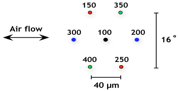
The layout of the patch of seven hairs as viewed from above. The numbers are the heights of the hairs in μm. The color coding identifies hairs of similar height in symmetric positions with respect to the oscillating hair flow.

The results from this simulation are pictured in Figure 8. Figure 8.A plots the coupling coefficient κ against frequency. We find that hair response to near neighbors is not linearly related to hair length, since intermediate hairs were the most affected by the presence of other hairs. The hairs of intermediate length experience an amplitude change of 75% to nearly 100%, whereas the shortest and longest hairs have their amplitudes damped by 59% to 70%. One possible explanation is that individual hair response is more dependent on position within a group of hairs than on hair length. There is some limited evidence for this hypothesis. The color coding in Figure 7 denotes hairs in symmetric positions within the group that have similar lengths. These “most similar” pairs have roughly parallel, close-set curves in Figure 8.A, although the trend is not repeated in Figure 8.B except for the longest pair of hairs. This suggests that position within a group of hairs along with coarsely quantized hair length may be the best predictor of viscous coupling effects.

Figure 8.

Change in hair response when individual hairs are simulated in a group. The hair lengths are listed in the legend; other hair parameters are calculated according to allometric relationships, see equations (10), (11), and (12); the peak air flow is 5 cm/s; the cercal diameter is 500μm; and the discretization scheme is described in the text. A. The coupling coefficient κ introduced in equation (26) vs frequency. B. The difference in phase shift (degrees) between isolated and grouped hairs as a function of frequency.

Figure 8.B plots the change in phase between the isolated and grouped hairs, θ_ref − θ. We cannot distinguish phase differences smaller than 4.5° because our time steps are 1/80 of a period apart. Also, phase shifts that differ by only 4.5° are likely numerical artifacts, so the non-smoothness in the phase graphs caused by 4.5° jumps should be ignored. Again, the intermediate length hairs are most affected by the presence of near neighbors. Interestingly, the 200 μm hair is phase-shifted nearly π radians at low frequencies, which suggests that a significant stagnation in the air flow can occur in a dense forest of hairs.

6 Conclusions

We have developed a framework that allows us to model and quantify the interaction between filiform hairs, which is mediated by the fluid medium. Our results demonstrate that the interaction between hairs in a group is substantial at biologically relevant distances, lengths of hairs and air velocities. In principle, we can extend our current modeling capability from a small cercal patch to the entire array of hairs on the cercus in periodic air flow. Modeling the whole cercus is a crucial step in our investigation of the function of the cercal sensory system of the cricket. We are interested in how the information about the air currents is represented by the motion of the filiform hairs, translated into the neural activity of the hair-attached afferent neurons and processed by the small set of interneurons in the terminal ganglion, before being passed on to higher processing stages. Apart from understanding the entire information pathway, we are also interested in uncovering operational principles that may be common with those in the auditory system in humans, or may be applicable to design of MEMS-based hair flow-sensors [19]. Since the cercal system evolved under the physical constraints imposed by the interaction with air at a low Reynolds number, it is likely that its operational characteristics reflect these constraints. We believe that the modeling framework presented in this paper will allow the simulation of a significant portion of the cercal sensory system and thus help us uncover these constraints.

A Scaling

In this appendix, we rescale the system of equations in Section 4.2. Let T be a time scale and L be a length scale. Define the dimensionless variables t̂, x̂ and r̂ by

$$\widehat{t}=\frac{1}{T}t,\widehat{\mathit{x}}=\frac{1}{L}\mathit{x},\widehat{r}=\frac{1}{L}r.$$

Recall that t is time, x is position and r is the magnitude of x. These choices for scaling terms define a velocity scale given by U = L/T such that a dimensionless velocity is û = (T/L)u. For convenience define dimensionless pressure and force as

$$\widehat{p}=\frac{1}{P}p,\widehat{\mathbf{F}}=\frac{1}{F}\mathbf{F}$$

We choose T = 1/f = 2π/ω so that the dimensionless period of oscillation of the hair and the far-field flow is 1. We select the length scale L to be the length of the longest hair. We set the pressure scale to be P = μ/T and choose F = I_s/T², where $I_s:={max}_{i,j}(m_j^{(i)}{r}_j^{(i)})$ is the maximum of the inertial factors over all positions on all hairs. These choices for scaling terms lead to a natural scaling for mass, $\widehat{m}=\frac{L}{F{T}^2}m=\frac{L}{I_s}m$, for inertia, $\widehat{I}=\frac{I}{I_{s}L}$, and for the inertial force constants, $\widehat{m}\widehat{r}=\frac{mr}{I_s}$.

With these choices the equation for the resistive forces has the form

$${\widehat{\mathbf{F}}}_{\mathit{IRS},j}^{(i)}=-{\widehat{m}}_j^{(i)}{\widehat{r}}_j^{(i)}\left[\left({{\theta }^{″}}^{(i)}(\widehat{t})+\frac{R^{(i)}T}{I^{(i)}}{{\theta }^{\prime }}^{(i)}(\widehat{t})+\frac{S^{(i)}{T}^2}{I^{(i)}}{\theta }^{(i)}(\widehat{t})\right){\mathbf{h}}^{(i)}+\mid {{\theta }^{\prime }}^{(i)}(\widehat{t}){\mid }^2{\mathbf{r}}^{(i)}\right].$$

The boundary layer equation in dimensionless form is given by

$${\widehat{\mathbf{u}}}_b=\frac{T}{L}{U}_0{B}_c(T\widehat{t},L\widehat{\mathit{x}})=\frac{2\pi }{L\omega }{U}_0{B}_c(2\pi \widehat{t}/\omega ,L\widehat{\mathit{x}}),$$

and the total scaled velocity is the sum of the scaled perturbation velocities and the scaled boundary layer, v̂ = û + û_b, where the scaled version of u is derived below.

We scale the Stokes equation, where

$$\mathbf{F}:=\sum _{i=1}^N{\mathbf{F}}_{\mathit{IRS}}^{(i)}+\sum _{\begin{array}{l}j=1\\ j\ne i\end{array}}^N{\mathbf{F}}_{\mathit{con}}^{(i)}+{\mathbf{F}}_{bc}^{(\mathcal{P})}.$$

Note that the Laplacian is scaled by 1/L², the gradient by 1/L, and φ_δ̂= L³φ_δ, because our particular choice of φ_δ has units (length)⁻³. Therefore the first equation has the form

$$\mathrm{\Delta }\widehat{\mathbf{u}}=\frac{PT}{\mu }\nabla \widehat{p}-\frac{FT}{L^2\mu }\widehat{\mathbf{F}}{\phi }_{\widehat{\delta }}=\nabla \widehat{p}-C_F\widehat{\mathbf{F}}{\phi }_{\widehat{\delta }}$$ (A.1)

where we set $C_F:=\frac{FT}{L^2\mu }=\frac{I_s\omega }{2\pi L^2\mu }$. Repeating the calculations in Section 2.2 with expression (A.1) and using ∇·û = 0, we observe that the constant C_F factors out of the matrix equation:

$$\widehat{\mathbf{u}}=C_{F}M\widehat{\mathbf{F}}.$$

Thus, the scaled inverse problem is

$$\widehat{\mathbf{F}}=\frac{1}{C_F}{M}^{-1}\widehat{\mathbf{u}}.$$

And the angular velocity equation scales to be

$${{\theta }^{\prime }}^{(i)}(\widehat{t})=\frac{{\sum }_{k=1}^{n_i}({\widehat{\mathbf{x}}}_k^{(i)}\times {\widehat{m}}_k^{(i)}{\widehat{\mathbf{v}}}_k^{(i)})·{\mathbf{n}}^{(i)}}{{\widehat{I}}^{(i)}}$$

Therefore, the our scaled equations are as follows:

$$\begin{array}{l}\mathrm{\Delta }\widehat{\mathbf{u}}=\nabla \widehat{p}-C_F\widehat{\mathbf{F}}{\phi }_{\widehat{\delta }}\\ \nabla ·\widehat{\mathbf{u}}=0\\ {\widehat{\mathbf{u}}}_b=\frac{2\pi }{L\omega }{U}_0{B}_c(2\pi \widehat{t}/\omega ,L\widehat{\mathit{x}})\\ {{\theta }^{\prime }}^{(i)}(\widehat{t})=\frac{{\sum }_{k=1}^{n_i}\left({\widehat{\mathbf{x}}}_k^{(i)}\times {\widehat{m}}_k^{(i)}{\widehat{\mathbf{v}}}_k^{(i)}\right)·{\mathbf{n}}^{(i)}}{{\widehat{I}}^{(i)}}\end{array}$$ (A.2)

$$\begin{array}{l}{\widehat{\mathbf{F}}}_{\mathit{IRS},j}^{(i)}=-{\widehat{m}}_j^{(i)}{\widehat{r}}_j^{(i)}\left[\left({{\theta }^{″}}^{(i)}(\widehat{t})+\frac{R^{(i)}T}{I^{(i)}}{{\theta }^{\prime }}^{(i)}(\widehat{t})+\frac{S^{(i)}{T}^2}{I^{(i)}}{\theta }^{(i)}(\widehat{t})\right){\mathbf{h}}^{(i)}+\mid {{\theta }^{\prime }}^{(i)}(\widehat{t}){\mid }^2{\mathbf{r}}^{(i)}\right]\\ {\widehat{\mathbf{F}}}_{\mathit{con}}^{(i)}=-\frac{1}{C_F}{(M^{(i,i)})}^{-1}({\widehat{\mathbf{v}}}^{(i)}-{\stackrel{.}{\theta }}^{(i)}(\widehat{t}){\widehat{\mathbf{r}}}_h^{(i)})\end{array}$$ (A.3)

$${\widehat{\mathbf{F}}}_{bc}^{(\mathcal{P})}=-\frac{1}{C_F}{(M^{(\mathcal{P})})}^{-1}({\widehat{\mathbf{u}}}^{(\mathcal{P})}).$$ (A.4)

B Solving for Angular Acceleration

In this appendix, we solve the system of equations in Section 4.2 for θ̈^(j) j = 1, …, N. Using (25) we write (24) as

$${\stackrel{.}{\theta }}^{(i)}=\frac{{\sum }_{k=1}^{n_i}({\mathbf{x}}_k^{(i)}\times m_k^{(i)}({\mathbf{u}}_{\mathit{IRS},k}^{(i)}+{\mathbf{u}}_{\mathit{con},k}^{(i)}+{\mathbf{u}}_{bc,k}^{(i)}+{\mathbf{u}}_{b,k}^{(i)}))·{\mathbf{n}}^{(i)}}{I^{(i)}},i=1,\dots ,N.$$ (B.1)

Observe that

$${\mathbf{u}}_{\mathit{IRS}}^{(i)}=\sum _{j=1}^N{M}^{(i,j)}\left({\ddot{\theta }}^{(j)}{\mathbf{C}}_I^{(j)}\right)+\sum _{j=1}^N{M}^{(i,j)}{\mathbf{F}}_{\mathit{rest}}^{(j)}=\sum _{j=1}^N{\ddot{\theta }}^{(j)}\left(M^{(i,j)}{\mathbf{C}}_I^{(j)}\right)+\sum _{j=1}^N{M}^{(i,j)}{\mathbf{F}}_{\mathit{rest}}^{(j)},$$

where ${\mathbf{C}}_I^{(j)}$ is a concatenation of the terms $-m_{\ell }^{(j)}{r}_{\ell }^{(j)}$ for all the points ℓ along hair j and ${\mathbf{F}}_{\mathit{rest}}^{(j)}={\mathbf{F}}_R^{(j)}+{\mathbf{F}}_S^{(j)}+{\mathbf{F}}_{\mathit{cent}}^{(j)}$ (these force terms are also concatenations along hair j).

The velocity ${\mathbf{u}}_{\mathit{con}}^{(i)}$, caused by the collection of forces F_con, is

$${\mathbf{u}}_{\mathit{con}}^{(i)}=\sum _{\begin{array}{l}j=1\\ j\ne i\end{array}}^N{M}^{(i,l)}{\mathbf{F}}_{\mathit{con}}^{(l)}.$$

Since by (20) ${\mathbf{F}}_{\mathit{con}}^{(l)}=-{(M^{(l,l)})}^{-1}({\mathbf{v}}^{(l)}-{\stackrel{.}{\theta }}^{(l)}{\mathbf{r}}_h^{(l)})$ we obtain

$${\mathbf{u}}_{\mathit{con}}^{(i)}=-\sum _{l=1}^N{M}^{(i,l)}{(M^{(l,l)})}^{-1}({\mathbf{v}}^{(l)}-{\stackrel{.}{\theta }}^{(l)}{\mathbf{r}}_h^{(l)}).$$ (B.2)

Using the simplifying assumptions in Section 4.2, the velocity ${\mathbf{u}}_{\mathit{con}}^{(i)}$ will be given by

$$\begin{array}{l}{\mathbf{u}}_{\mathit{con}}^{(i)}=-\sum _{\begin{array}{l}l=1\\ l\ne i\end{array}}^N{M}^{(i,l)}{(M^{(l,l)})}^{-1}\left({\mathbf{u}}_{\mathit{IRS}}^{(l)}+{\mathbf{u}}_b^{(l)}-{\stackrel{.}{\theta }}^{(l)}{\mathbf{r}}_h^{(l)}\right)\\ =-\sum _{\begin{array}{l}l=1\\ l\ne i\end{array}}^N{M}^{(i,l)}{(M^{(l,l)})}^{-1}\left(\sum _{j=1}^N{\ddot{\theta }}^{(j)}\left(M^{(l,j)}{\mathbf{C}}_I^{(j)}\right)+\sum _{j=1}^N{M}^{(l,j)}{\mathbf{F}}_{\mathit{rest}}^{(j)}+{\mathbf{u}}_b^{(l)}-{\stackrel{.}{\theta }}^{(l)}{\mathbf{r}}_h^{(l)}\right)\\ =-\sum _{\begin{array}{l}l=1\\ l\ne i\end{array}}^N{M}^{(i,l)}{(M^{(l,l)})}^{-1}\left(\sum _{j=1}^N{\ddot{\theta }}^{(j)}(M^{(l,j)}{\mathbf{C}}_I^{(j)})\right)\\ -\sum _{\begin{array}{l}l=1\\ l\ne i\end{array}}^N{M}^{(i,l)}{(M^{(l,l)})}^{-1}\left(\sum _{j=1}^N{M}^{(l,j)}{\mathbf{F}}_{\mathit{rest}}^{(j)}+{\mathbf{u}}_b^{(l)}-{\stackrel{.}{\theta }}^{(l)}{\mathbf{r}}_h^{(l)}\right)\\ =-\sum _{j=1}^N{\ddot{\theta }}^{(j)}\sum _{\begin{array}{l}l=1\\ l\ne i\end{array}}^N{M}^{(i,l)}{(M^{(l,l)})}^{-1}\left(M^{(l,j)}{\mathbf{C}}_I^{(j)}\right)-{\mathit{f}}^{(i)}\end{array}$$

where we defined

$${\mathit{f}}^{(i)}:=\sum _{\begin{array}{l}l=1\\ l\ne i\end{array}}^N{M}^{(i,l)}{(M^{(l,l)})}^{-1}\left(\sum _{j=1}^N{M}^{(l,j)}{\mathbf{F}}_{\mathit{rest}}^{(j)}+{\mathbf{u}}_b^{(l)}-{\stackrel{.}{\theta }}^{(l)}{\mathbf{r}}_h^{(l)}\right).$$

Again using the simplifying assumptions in Section 4.2, we compute ${\mathbf{u}}_{bc}^{(i)}$

$$\begin{array}{l}{\mathbf{u}}_{bc}^{(i)}=M^{(i,\mathcal{P})}{(M^{(\mathcal{P},\mathcal{P})})}^{-1}\left(-{\mathbf{u}}_{\mathit{IRS}}^{(\mathcal{P})}\right)\\ =M^{(i,\mathcal{P})}{(M^{(\mathcal{P},\mathcal{P})})}^{-1}\left(-\sum _{j=1}^N{\ddot{\theta }}^{(j)}\left(M^{(\mathcal{P},j)}{\mathbf{C}}_I^{(j)}\right)-\sum _{j=1}^N{M}^{(\mathcal{P},j)}{\mathbf{F}}_{\mathit{rest}}^{(j)}\right)\\ =\sum _{j=1}^N{\ddot{\theta }}^{(j)}{M}^{(i,\mathcal{P})}{(M^{(\mathcal{P},\mathcal{P})})}^{-1}\left(-M^{(\mathcal{P},j)}{\mathbf{C}}_I^{(j)}\right)+{\mathit{g}}^{(i)}\end{array}$$

where we defined

$${\mathit{g}}^{(i)}:=M^{(i,\mathcal{P})}{(M^{(\mathcal{P},\mathcal{P})})}^{-1}\left(-\sum _{j=1}^N{M}^{(\mathcal{P},j)}{\mathbf{F}}_{\mathit{rest}}^{(j)}\right).$$

To simplify, let

$$\begin{array}{l}{\mathbf{a}}^{(i,k)}:=M^{(i,k)}{\mathbf{C}}_I^{(k)}\\ {\mathbf{b}}^{(i,k)}:=\sum _{l=1}^N{M}^{(i,l)}{(M^{(l,l)})}^{-1}\left(M^{(l,k)}{\mathbf{C}}_I^{(k)}\right)\\ {\mathbf{c}}^{(i)}:=\sum _{j=1}^N{M}^{(i,j)}{\mathbf{F}}_{\mathit{rest}}^{(j)}-{\mathit{f}}^{(i)}+{\mathit{g}}^{(i)}+{\mathit{u}}_b^{(i)}\end{array}$$

Then,

$$\begin{array}{l}{\mathbf{v}}^{(i)}={\mathit{u}}_{\mathit{IRS}}^{(i)}+{\mathit{u}}_{\mathit{con}}^{(i)}+{\mathit{u}}_{bc}^{(i)}+{\mathit{u}}_b^{(i)}\\ =\sum _{j=1}^N{\ddot{\theta }}^{(j)}\left({\mathbf{a}}^{(i,j)}-{\mathit{b}}^{(i,j)}-M^{(i,\mathcal{P})}{(M^{(\mathcal{P},\mathcal{P})})}^{-1}{\mathit{a}}^{(\mathcal{P},j)}\right)+{\mathit{c}}^{(i)}.\end{array}$$

Substituting into the original equation (B.1) we are left with

$$\begin{array}{l}{\stackrel{.}{\theta }}^{(i)}=\frac{{\sum }_{k=1}^{n_i}{\mathit{x}}_k^{(i)}\times m_k^{(i)}\left({\sum }_{j=1}^N{\ddot{\theta }}^{(j)}({\mathit{a}}^{(i,j)}-{\mathit{b}}^{(i,j)}-M^{(i,\mathcal{P})}{(M^{(\mathcal{P},\mathcal{P})})}^{-1}{\mathit{a}}^{(\mathcal{P},j)})+{\mathit{c}}^{(i)}\right)}{I^{(i)}}·{\mathit{n}}^{(i)}\\ =\sum _{j=1}^N{\ddot{\theta }}^{(j)}\left(\frac{{\sum }_{k=1}^{n_i}{\mathit{x}}_k^{(i)}\times m_k^{(i)}({\mathit{a}}^{(i,j)}-{\mathit{b}}^{(i,j)}-M^{(i,\mathcal{P})}{(M^{(\mathcal{P},\mathcal{P})})}^{-1}{\mathit{a}}^{(\mathcal{P},j)})}{I^{(i)}}·{\mathit{n}}^{(i)}\right)\\ +\frac{{\sum }_{k=1}^{n_i}{\mathit{x}}_k^{(i)}\times m_k^{(i)}{\mathit{c}}^{(i)}}{I^{(i)}}·{\mathit{n}}^{(i)}\\ =:\sum _{j=1}^N{A}_{ij}{\ddot{\theta }}^{(j)}+B_i\end{array}$$

where A_ij and B_i are defined as follows

$$A_{ij}:=\left(\frac{{\sum }_{k=1}^{n_i}{\mathit{x}}_k^{(i)}\times m_k^{(i)}({\mathit{a}}^{(i,j)}-{\mathit{b}}^{(i,j)}-M^{(i,\mathcal{P})}{(M^{(\mathcal{P},\mathcal{P})})}^{-1}{\mathit{a}}^{(\mathcal{P},j)})}{I^{(i)}}·{\mathit{n}}^{(i)}\right)$$

and

$$B_i:=\frac{{\sum }_{k=1}^{n_i}{\mathit{x}}_k^{(i)}\times m_k^{(i)}{\mathit{c}}^{(i)}}{I^{(i)}}·{\mathit{n}}^{(i)}.$$

Let A be a matrix with elements A_ij and b a vector with elements θ̇⁽ⁱ⁾ − B_i. Then (B.1) can be written as a system

$$A\ddot{\mathit{\theta }}=\mathit{b}.$$

References

- 1.Bacon JP, Murphey RK. Receptive fields of cricket (Acheta domesticus) are determined by their dendritic structure. J Physiol (Lond) 1984;352:601–613. doi: 10.1113/jphysiol.1984.sp015312. [DOI] [PMC free article] [PubMed] [Google Scholar]
- 2.Batchelor GK. An Introduction to Fluid Dynamics. Cambridge University Press; 2000. [Google Scholar]
- 3.Bathellier B, Barth FG, Albert JT, Humphrey JAC. Viscosity-mediated motion coupling between pair of trichobothria on the leg of the spider Cupiennius salei. J Comp Physiol A. 2005;191:733–746. doi: 10.1007/s00359-005-0629-5. [DOI] [PubMed] [Google Scholar]
- 4.Boyan GS, Ashman S, BallAshman EE. Initiation and modulation of flight by a single giant interneuron in the cercal system of the locust. Naturwissenschaften. 1986;73:272–274. [Google Scholar]
- 5.Camhi JM. The escape system of the cockroach. Scientific American. 1980;243:144–157. [Google Scholar]
- 6.Cortez R, Fauci L, Medovikov A. The method of regularized stokeslets in three dimensions: Analysis, validation, and application to helical swimming. Physics of Fluids. 2005;17:031504. [Google Scholar]
- 7.Cortez R. The method of regularized stokeslets. SIAM J Sci Comput. 2001;23:1204–1225. [Google Scholar]
- 8.Gnatzy, Heusslein Digger wasp against crickets. I. Receptors involved in the antipredator strategies of the prey. Naturwissenschaften. 1986;73:212–215. [Google Scholar]
- 9.Heinzel HG, Dambach M. Traveling air vortex rings as potential communication signals in a cricket. J Comp Physiolo A. 1987;160:79–88. [Google Scholar]
- 10.Hoyle G. The leap of the grasshopper. Sci Am. 1958;198:30–35. [Google Scholar]
- 11.Huber F, Moore TH, Loher W. Cricket Behavior and Neurobiology. Cornell University Press; 1989. [Google Scholar]
- 12.Humphrey J, Devarekonda R, Iglesias I, Barth FG. Dynamics of arthropod filiform hairs. I. Mathamatical modelling of the hair and air motions. Phil Trans R Soc Lond B. 1993;340:423–444. [Google Scholar]
- 13.Jacobs GA, Miller JP, Murphy RK. Cellular mechanisms underlying directional sensitivity of an identified sensory interneuron. J Neuroscience. 1986;6:2298–2311. doi: 10.1523/JNEUROSCI.06-08-02298.1986. [DOI] [PMC free article] [PubMed] [Google Scholar]
- 14.Jacobs GA, Nevin R. Anatomical relationship between sensory afferent arborizations in the cricket cercal system. Anat Rec. 1991;231:563–572. doi: 10.1002/ar.1092310418. [DOI] [PubMed] [Google Scholar]
- 15.Jacobs GA, Theunissen F. Functional organization of a neural map in the cricket cercal sensory system. J Neurosci. 1996;16:769–784. doi: 10.1523/JNEUROSCI.16-02-00769.1996. [DOI] [PMC free article] [PubMed] [Google Scholar]
- 16.Jacobs GA, Theunissen F. Extraction of sensory parameters from a neural map by primary sensory interneurons. J Neurosci. 2000;20:2934–2943. doi: 10.1523/JNEUROSCI.20-08-02934.2000. [DOI] [PMC free article] [PubMed] [Google Scholar]
- 17.Kamper G, Kleindienst H-U. Oscillation of cricket sensory hairs in a low frequency sound field. J Comp Physiol A. 1990;167:193–200. [Google Scholar]
- 18.Kanou M, Shimozawa TA. Threshold analysis of cricket cercal interneurons by an alternating air-current stimulus. J Comp Physiol A. 1984;154:357–365. [Google Scholar]
- 19.Krijnen G, Dijkstra M, van Baar J, Shankar S, Kuipers W, de Boer R, Altpeter D, Lammering T, Wiegering R. MEMS based hair flow-sensors as model systems for acoustic perception studies. Nanotechnology. 2006;17:S84–S89. doi: 10.1088/0957-4484/17/4/013. [DOI] [PubMed] [Google Scholar]
- 20.Kumagai T, Shimozawa TA, Baba Y. Mobilities of the cercal wind-receptor hairs of the cricket. J Comp Physiol A. 1998;183:7–21. [Google Scholar]
- 21.Kumagai T, Shimozawa TA, Baba Y. The shape of wind-receptor hairs of cricket and cockroach. J Comp Physiol A. 1998;183:187–192. [Google Scholar]
- 22.Landau LD, Lifschitz EM. Fluid Mechanics. Pergamon Press; 1959. [Google Scholar]
- 23.Landolfa MA, Jacobs GA. Direction sensitivity of the filiform hair population of the cricket cercal system. J Com Physiol A. 1995;177:759–766. [Google Scholar]
- 24.Landolfa MA, Miller JP. Stimulus-response properties of cricket cercal filiform hair receptors. J Com Physiol A. 1995;177:749–757. [Google Scholar]
- 25.Magal C, Dangles O, Caparroy P, Casas J. Hair canopy of cricket sensory system tuned to predator signals. J Theor Biol. 2006;241:459–466. doi: 10.1016/j.jtbi.2005.12.009. [DOI] [PubMed] [Google Scholar]
- 26.Miller JP, Jacobs GA, Theunissen FE. Representation of sensory information in the cricket cercal sensory system. I. Response properties of the primary interneurons. J Neurophys. 1991;66:1680–1689. doi: 10.1152/jn.1991.66.5.1680. [DOI] [PubMed] [Google Scholar]
- 27.Osborne L. PhD thesis. University of California; 1996. Signal processing in mechanosensory array: dynamics of cricket cercal hairs. [Google Scholar]
- 28.Palka J, Levine R, Schubiger M. The cercus-to-giant interneuron system of crickets. I. Some aspects of the sensory cells. J Comp Physiol. 1977;119:267–283. [Google Scholar]
- 29.Paydar S, Doan C, Jacobs GA. Neural mapping of direction and frequency in the cricket cercal sensory system. J Neurosci. 1999;19:1771–1781. doi: 10.1523/JNEUROSCI.19-05-01771.1999. [DOI] [PMC free article] [PubMed] [Google Scholar]
- 30.Pozrikidis C. Introduction to Theoretical and Computational Fluid Dynamics. Oxford University Press; 1997. [Google Scholar]
- 31.Shimozawa T, Kanou M. The aerodynamics and sensory physiology of a range fractionation in the cercal filiform sensilla of the cricket Gryllus bimaculatus. J Comp Physiol A. 1984;155:495–505. [Google Scholar]
- 32.Shimozawa T, Kanou M. Varieties of filiform hairs: range fractionation by sensory afferents and cercal interneurons of a cricket. J Comp Physiol A. 1984;155:485–493. [Google Scholar]
- 33.Shimozawa T, Kumagai T, Baba Y. Structural scaling and functional design of the cercal wind-receptor hairs of cricket. J Comp Physiol A. 1998;183:171–186. [Google Scholar]
- 34.Steiner AL. Behavioral interactions between Lisra nigra Vander Linden (Hymenoptera:Sphecidae) and Gryllus domesticus L. (Orthoptera: Gryllidae) Psyche (Camb Mass) 1968;75:256–273. [Google Scholar]
- 35.Stokes GG. On the effect of the internal friction of fluids on the motion of pendulums. Trans Cambridge Philos Soc. 1851;9:8. [Google Scholar]
- 36.Stout JF, DeHaan CH, McGhee RW. Attractiveness of the male Acheta domesticus calling song to females. I. Dependence on each of the calling song features. J Comp Physiol. 1983;153:509–521. [Google Scholar]
- 37.Theunissen FE, Miller JP. Representation of sensory information in the cricket cercal sensory system. II. Information theoretic calculation of system accuracy and optimal tuning curve width of four primary interneurons. J Neurophysiol. 1991;66:1690–1703. doi: 10.1152/jn.1991.66.5.1690. [DOI] [PubMed] [Google Scholar]
- 38.Theunissen F, Roddey JC, Stuffebeam S, Clague H, Miller JP. Information theoretic analysis of dynamical encoding by four primary interneurons in the cricket cercal system. J Neurophysiol. 1996;75:1345–1364. doi: 10.1152/jn.1996.75.4.1345. [DOI] [PubMed] [Google Scholar]
- 39.Thurm U, Kuppers J. Epithelial physiology of insect sensilla. In: Locke M, Smith DS, editors. Insect Biology in the Future. Academic Press; New York: 1980. pp. 735–763. [Google Scholar]
- 40.Thurm U. Mechanoreceptors in the cuticle of the honey bee: Fine structure and stimulus mechanism. Science. 1964;145:1063–1065. doi: 10.1126/science.145.3636.1063. [DOI] [PubMed] [Google Scholar]
- 41.Thurm U. An insect mechanoreceptor. II. Receptor potentials. Cold Spring Harb Symp Quant Biol. 1965;30:83–94. doi: 10.1101/sqb.1965.030.01.012. [DOI] [PubMed] [Google Scholar]
- 42.Thurm U. An insect mechanoreceptor. I. Fine structure and adequate stimulus. Cold Spring Harb Symp Quant Biol. 1965;30:75–82. doi: 10.1101/sqb.1965.030.01.011. [DOI] [PubMed] [Google Scholar]
- 43.Thurm U. Mechano-electric transduction. In: Hoppe W, Lohmann W, Markl H, Ziegler H, editors. Biophysics. Springer-Verlag; Berlin: 1983. pp. 666–671. [Google Scholar]
- 44.Walthall WW, Murphey RK. Positional information, compartments and the cercal system of crickets. Dev Biol. 1986;113:182–200. [Google Scholar]