Estimation and inference for case–control studies with multiple non–gold standard exposure assessments: with an occupational health application

Abstract

In occupational case–control studies, work-related exposure assessments are often fallible measures of the true underlying exposure. In lieu of a gold standard, often more than 2 imperfect measurements (e.g. triads) are used to assess exposure. While methods exist to assess the diagnostic accuracy in the absence of a gold standard, these methods are infrequently used to correct for measurement error in exposure–disease associations in occupational case–control studies. Here, we present a likelihood-based approach that (a) provides evidence regarding whether the misclassification of tests is differential or nondifferential; (b) provides evidence whether the misclassification of tests is independent or dependent conditional on latent exposure status, and (c) estimates the measurement error–corrected exposure–disease association. These approaches use information from all imperfect assessments simultaneously in a unified manner, which in turn can provide a more accurate estimate of exposure–disease association than that based on individual assessments. The performance of this method is investigated through simulation studies and applied to the National Occupational Hazard Survey, a case–control study assessing the association between asbestos exposure and mesothelioma.

1. INTRODUCTION

Mismeasurement of exposure, disease, or covariates is ubiquitous in epidemiological research (Cole and others, 2006). Many quantitative methods have been proposed to correct misclassification bias, most of which utilize additional information to reconstruct the relation between observed measurements and true values. Examples of these methods include regression calibration and multiple imputation (Rosner and others, 1989; Spiegelman and others, 1997, Spiegelman and others, 2001; Chu and Halloran, 2004; Chu and others, 2006), in which the connection is often reconstructed based on a validation study in a subset of the observed participants, and sensitivity analysis (Greenland, 1996, Greenland, 2005), in which the connection is reconstructed based on prior information or expert opinion. In population-based case–control studies attempting to assess an association between work-related exposures and disease, exposure levels are often derived by interviews conducted to collect detailed information on the employment history and other factors that would affect exposure of cases and controls (Daniels and others, 2001; Nam and others, 2005). Gold standard measurements are typically not available. In the absence of a gold standard, it is common to apply 2 or more imperfect measurements to evaluate exposure status.

A considerable literature is available on the methodological approaches to assess the accuracy of multiple binary measurements, which is usually quantified using sensitivity and specificity (Gart and Buck, 1966; Hui and Walter, 1980; Joseph and others, 1995; Andersen, 1997; Johnson and others, 2001). When the exposure status is subject to misclassification (as in many case–control studies due to imperfect recall), sensitivity is defined as the probability of testing positive for exposure given truly exposed and specificity is defined as the probability of testing negative for exposure given truly nonexposed (Zhou and others, 2002; Pepe, 2003). Using the framework of a Hui–Walter design (Hui and Walter, 1980), the sensitivities and specificities of each imperfect measurement can be estimated without ascertaining the true exposure status under conditional independence of testing results given underlying exposure status.

When the conditional independence assumption is falsely assumed, parameter estimates are biased (Vacek, 1985). Several models have been proposed to incorporate dependence across multiple imperfect measurements, which include a log-linear modeling approach (Espeland and Handelman, 1989), a Gaussian random-effects model (Qu and others, 1996), and a finite mixture model (Albert and others, 2001). Furthermore, Albert and Dodd (2004) reported that when the conditional dependence between imperfect measurements is misspecified, estimators of sensitivity, specificity, and prevalence may be biased and suggested a large number (≥ 10) of imperfect measurements (or repeated measurements) to distinguish between models accounting for dependence, which is usually unavailable. When multiple or repeated imperfect measurements were used to assess exposure status in case–control studies, nondifferential misclassification (i.e. measurement error rates are the same for cases and controls) was commonly assumed (Satten and Kupper, 1993; Lai and others, 2007). However, in some occupational health and epidemiological case–control studies, differential misclassification of exposure status is likely due to differential recall and such differential misclassification can cause bias of unknown direction for the exposure–disease association (Greenland, 1996, Greenland, 2005). Although many methods for handling misclassified exposure in case–control studies have been proposed, to our knowledge, methods for simultaneously accounting for conditional dependence and differential misclassification have not been previously described.

In this paper, we discuss statistical inference and study the performance of a likelihood-based frequentist approach to estimate the measurement error–corrected exposure–disease association in case–control studies. We focus on the special case where 3 tests are available. For this special case, Pepe and Janes (2007) have recently derived closed-form expressions for the maximum likelihood estimators (MLEs) under the conditional independence assumption and provided some insights into latent class analysis of diagnostic test performance with a single homogenous group of subjects. Our focus here is on the impact of misspecification of differential/nondifferential misclassification of exposure status and/or conditional independent/dependent misclassification on the estimators of the exposure–disease association for a case–control study. In Section 2, we provide a motivating case–control study to assess the association between asbestos exposure and mesothelioma (Nam and others, 2005). In Section 3, we present a likelihood-based approach to estimate the measurement error–corrected exposure–disease association. In Section 4, we describe the results for the motivating example as presented in Section 2. A set of simulation studies is presented in Section 5 to investigate the performance of the proposed approach. A discussion is presented in Section 6.

2. STUDY BACKGROUND

A case–control study was conducted to assess the association between asbestos exposure and mesothelioma from the National Occupational Hazard Survey (Nam and others, 2005). Cases were selected from 3 sources between 1975 and 1980: the New York State Health Department Cancer Registry, the Los Angeles County Cancer Surveillance Program, and 39 Veterans Administration (VA) Hospitals. Controls were selected from the same geographical area (New York, Los Angeles) or the same hospital (VA). Table 1 presents the frequency of the number of participants cross tabulated by the 3 assessment methods as well as the case–control status. Exposure assessment was conducted in 3 ways. First, next-of-kin respondents were contacted to provide reports of occupational exposure. Second, work histories were classified using a job exposure matrix. Third, an occupational hygienist classified each case and control based on work histories. The odds ratios (OR) of mesothelioma for those with and without the asbestos exposure assessed by the 3 exposure assessment methods were estimated to be 10.74 (95% confidence limits [CL]: 7.27, 15.90), 4.65 (95% CL: 3.19, 6.77), and 2.06 (95% CL: 1.48, 2.86), respectively. However, none of these estimates likely reflect the true association between asbestos exposure and mesothelioma due to potential nondifferential or differential and independent or dependent misclassification of asbestos exposure. Moreover, in this case–control setting, differential misclassification of exposure status is possible. For instance, surviving family members may be more likely to ascribe a death due to lung disease to possible workplace exposures than other deaths, which can cause bias of unknown direction (Greenland, 1996, Greenland, 2005).

Table 1.

A case–control study of asbestos and mesothelioma from the National Occupational Hazard Survey

Exposure test positive (+) or negative (–)			Number of subjects
Next-of-kin respondents (X1)	Expert assessment (X2)	Job exposure matrix (X3)	Cases (D = 1)	Controls (D = 0)
+	+	+	69	36
+	+	–	47	14
+	–	+	0	4
+	–	–	1	3
–	+	+	22	82
–	+	–	28	113
–	–	+	7	39
–	–	–	34	242
	Total		208	533

3. STATISTICAL METHODS

Let D represent the disease status with 1 denoting a case and 0 indicating a control. Let E represent the true exposure status with 1 being exposed and 0 being unexposed. Let π_d be the probability of being truly exposed and n_d be the number of participants in the dth disease group. Let X_dji represent the classification of the jth test $(j=1,2,\dots ,J)$ with a value 1 indicating test positive and 0 indicating test negative on the ith subject $(i=1,2,\dots ,n_d)$ in the dth disease group. For the estimation of exposure–disease association, we used a logistic regression model $\text{logit}\left({\pi }_d\right)={\eta }_0+{\eta }_{1}d$ to relate the probability of being exposed to disease status D. For the relationship between imperfect measurements and true exposure status, in principle, we allow differential (i.e. the sensitivity or the specificity of a test can differ for cases and controls) and/or conditional dependent misclassification (i.e. the imperfect measurements can be correlated conditioning on the latent exposure status). Specifically, the positive classification probability for the ith subject in the dth disease group by the jth test is assumed to be dependent on the disease status D, the exposure status E, and a Gaussian latent variable Z, through a generalized linear regression model, such as a probit model (Qu and others, 1996; Qu and Hadgu, 1998):

(3.1)

where d = 0, 1, e = 0, 1,and Z∼ N(0, 1). As commonly done in latent variable modeling, we assume that the Gaussian latent variable Z is independent of the disease status D. The Gaussian latent variable Z captures the dependence or similarity among multiple error-prone exposure measurements conditioning on the unmeasured true exposure status.

Let Se_dj and Sp_dj denote the sensitivity and specificity for the dth group (d = 0, 1) and the jth diagnostic test. Nondifferential misclassification corresponds to ${\text{Se}}_{0j}={\text{Se}}_{1j}={\text{Se}}_j$ and ${\text{Sp}}_{0j}={Sp}_{1j}={Sp}_j$, or equivalently ${\alpha }_{1ej}=0\left(e=0,1\right)$ for $j=1,2,\dots ,J$. The population-averaged sensitivity and specificity of the jth test are

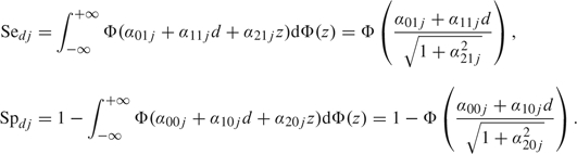(3.2)

The probability of observing subjects with $X_1=x_1$, $X_2=x_2$, …, and $X_J=x_j$ in the dth disease group $P_d\left(\text{x}\right)$ is

(3.3)

Let $n_d\left(\text{x}\right)$ be the number of subjects in the dth disease group classified by exposure assessment as the vector $\text{x}=\left(x_1,x_2,\dots ,x_J\right)$. The log-likelihood function for θ = (η_d,α_kej), where $k=0,1,2,d=0,1$, and $j=1,2,$ …, J, is the summation of the contribution from each category, that is

(3.4)

To test whether the misclassification by an exposure assessment procedure j is nondifferential or differential by disease status D or to test whether the misclassification of a test is independent of the others conditioning on exposure status E, the likelihood ratio test (LRT) can be used to test whether ${\alpha }_{1ej}=0$ or ${\alpha }_{2ej}=0$ for $e=0,1$ and $j=1,2,\dots ,J$. To reduce the possibility of failure to detect differential misclassification due to lack of power, if the null hypothesis is not rejected at a conservative cutoff point of P-value (e.g. 0.10), nondifferential sensitivity/specificity and/or conditional independence will be used in the probit model as in (3.1). The final model is compared to the saturated differential and/or conditional dependent misclassification model to test goodness of fit using the LRT.

If there are J binary diagnostic tests that classify exposure status for each participant, then there are $2^J$ possible combinations of classifications of exposure status. A full model in (3.1) has $6J+2$ independent parameters. For a fixed number of participants, there are $2^{J+1}-2$ degrees of freedom in a case–control design (i.e. the maximum number of parameters that can be estimated), which inhibits us exploring differential and conditional dependent misclassification simultaneously when $J\le 3$. When $J=2$, 6 parameters can be estimated, which only allows an estimation assuming nondifferential and conditional independent misclassification. In this special case, the closed-form MLEs were provided by Hui and Walter (1980). When $J=3$, only 14 parameters can be estimated, allowing for an exploration of either differential or conditional dependent misclassification, but not both. In other words, if both differential and conditional dependent misclassifications are of concern, $J=3$ measures only allow an exploration of some models under partial differential and constrained conditional dependent misclassification (e.g. ${\alpha }_{2ej}={\alpha }_{2e}$ for $e=0,1$ and $j=1,2,\dots ,J$). Assuming conditional independent and differential misclassification, the probit model is essentially nonparametric and saturated. The closed-form MLEs are directly available following the derivation of MLEs for a single group with 3 tests by Pepe and Janes (2007).

The probit regression models can be extended to incorporate the other covariates’ effects on the sensitivity, specificity, and the probability of being truly exposed. Here we concentrate on the impact of misspecification of differential/nondifferential and conditional independent/dependent misclassification on the estimators of exposure–disease association without additional covariates. The nonlinear random-effects model was fitted using PROC NLMIXED in SAS version 9.1 (SAS Institute Inc., Cary, NC), which maximizes an approximation to the likelihood integrated over the random effects (Pinheiro and Bates, 1995). An adaptive Gaussian quadrature approximation and dual quasi-Newton algorithm optimization techniques in PROC NLMIXED were used to maximize the approximate integrated likelihood. We used PROC NLMIXED built-in ability using the delta method to compute the population estimates of the back-transformed parameters of interest and their confidence intervals based on a normal approximation.

4. A CASE STUDY IN OCCUPATIONAL HEALTH

In this section, we present the results for the case study described in Section 2 using methods in Section 3. In this case study with $J=3$, a model with full differential and full conditional dependent misclassification is not identifiable, it is impossible to distinguish differential misclassification from conditional dependence. We use a somewhat ad hoc approach to select a “final” partial differential and constrained conditional dependence model. Specifically, we first select a “final” partial differential independent misclassification model based on an LRT. Then, we investigate some constrained conditional dependence structures on the “final” partial differential independent misclassification model that we selected.

Table 2 presents the estimates and their 95% CL using the maximum likelihood approach for 4 models. Models I, II, and III assume conditional independence. Specifically, Model I is a model that allows differential and conditional independent exposure misclassification for all 3 exposure assessments. Model II places constraints on Model I such that all 3 exposure assessments are assumed to be nondifferentially misclassified, which does not provide a good fit to the data compared to Model I (P-value  <  0.001). Model III is a compromise between Models I and III and was arrived via LRTs. It provides a good fit to the data compared to Model I (P-value = 0.156). In Model III, only the sensitivities of the next-of-kin reports and the job exposure matrix are allowed to be differential with respect to disease status; all 3 specificities and the sensitivity of occupational hygienist classifications were (appropriately, based on the data and model) constrained to be nondifferential. We term Model III as “a model with partially differential misclassification under conditional independence.” It was expected a priori that the measurement error for expert assessment would be nondifferential because the occupational hygienists who performed expert assessment did not have knowledge of disease status. It is often assumed that the next-of-kin reports may be subject to recall bias differential by disease status; therefore, differential measurement error for the next-of-kin reports is not surprising. Based on Model III, the next-of-kin reports had higher sensitivity when comparing cases versus controls (i.e. 0.77 vs. 0.36), while the job exposure matrix had lower sensitivity when comparing cases versus controls (i.e. 0.59 vs. 0.75). The measurement error–corrected OR was 7.47 (95% CL: 3.68, 11.30), which is noticeably different from any of the 3 single classifications of exposure.

Table 2.

Summary of parameter estimates and their 95% confidence intervals using maximum likelihood methods

	Conditional independent models			IV. Partially differential and conditional dependent model
	I. Differential	II. Nondifferential	III. Partially differential
Se01	0.337 (0.234, 0.441)	0.742 (0.621, 0.864)	0.358 (0.253, 0.462)	0.506 (0.197, 0.814)
Se11	0.784 (0.673, 0.895)		0.770 (0.687, 0.853)	0.820 (0.718, 0.921)
Sp01	0.993 (0.976, 1.000)	0.979 (0.954, 1.000)	0.983 (0.960, 1.000)	0.945 (0.930, 0.959)
Sp11	0.976 (0.930, 1.000)
Se02	0.905 (0.804, 1.000)	0.999 (0.952, 1.000)	0.986 (0.947, 1.000)	0.999 (0.977, 1.000)
Se12	1.000 (1.000, 1.000)
Sp02	0.734 (0.662, 0.806)	0.633 (0.575, 0.690)	0.723 (0.657, 0.790)	0.610 (0.554, 0.666)
Sp12	0.693 (0.463, 0.922)
Se03	0.728 (0.593, 0.863)	0.652 (0.582, 0.723)	0.752 (0.621, 0.883)	0.732 (0.510, 0.954)
Se13	0.596 (0.506, 0.687)		0.590 (0.506, 0.674)	0.583 (0.493, 0.673)
Sp03	0.883 (0.831, 0.936)	0.778 (0.729, 0.827)	0.855 (0.812, 0.899)	0.754 (0.712, 0.800)
Sp13	0.833 (0.721, 0.946)
OR	5.577 (1.898, 9.257)	14.580 (7.258, 21.901)	7.470 (3.962, 10.977)	16.124 (5.217, 27.031)
– 2logL	2294.70	2342.10	2301.3	2294.4
D.F.	—	6	4	5
P-value	—	< 0.001	0.159	—

Note: D.F., Degree of freedom; Se_dj and Sp_dj denote the sensitivity and specificity for the dth group (d = 1, 0 corresponding cases and controls, respectively) and the jth diagnostic test with 1 denoting the next-of-kin respondents, 2 denoting expert assessment, and 3 denoting job exposure matrix; P-values are based on the LRTs for goodness of fit.

To incorporate potential conditional dependence in the data analysis, we extended Model III to allow homogeneous conditional dependence on specificities or sensitivities or both (i.e. ${\alpha }_{2e1}={\alpha }_{2e2}={\alpha }_{2e3}={\alpha }_{2e}$ for $e=0,1)$. Only the inclusion of homogeneous conditional dependence on specificities significantly improved the goodness of fit (i.e. −2 log-likelihood = 2294.4, which is a little bit smaller than the −2 log-likelihood = 2294.7 under differential misclassification), and we term this model as Model IV, “a `final’ model” with partially differential and constrained conditional dependent exposure misclassification. The estimated α₂₀ is ₂₀ = 0.987 with a standard error of 0.138 (P-value  <  0.001). The Akaike information criterion for the 4 models are 2322.7, 2358.1, 2321.3, and 2316.4, respectively, also suggesting that the “final” model (Model IV) with partially differential and constrained conditional dependent exposure misclassification fits the data better. The population-averaged specificities using (3.2) were presented in Table 2. The measurement error–corrected OR was 16.12 (95% CL: 5.22, 27.03), which differs notably from the results based on the partial differential misclassification and conditional independent model, that is OR = 7.47 (95% CL: 3.68, 11.30), but it is very similar to the estimate under the nondifferential misclassification and conditional independent model, that is OR = 14.58 (95% CL: 7.26, 21.90).

5. SIMULATION STUDIES

Four sets of simulations with different levels of differential misclassification and conditional dependence were performed to evaluate the impact of potential misspecification of differential/nondifferential and conditional independent/dependent misclassification of exposure status on the estimation of exposure–disease association. For each set of simulations, 2000 replications were used. To reflect the case study presented in Section 2, 250 cases and 500 controls were generated for each simulated case–control study. Furthermore, the probabilities of true exposure were set to be 0.269 and 0.731 for the controls and cases, respectively, which corresponds to a log OR of 2.0 for the exposure–disease association. The sensitivities, that is (Se${}_{01}$, Se${}_{11}$, Se${}_{02}$, Se${}_{12}$, Se${}_{03}$, Se${}_{13})$, were set to be conditionally independent and either nondifferentially misclassified with values of (0.70, 0.70, 0.90, 0.90, 0.80, 0.80) or differentially misclassified with values of (0.80, 0.50, 0.90, 0.90, 0.80, 0.80). The specificities, that is (Sp${}_{01}$, Sp${}_{11}$, Sp${}_{02}$, Sp${}_{12}$, Sp${}_{03}$, Sp${}_{13})$, were set to be nondifferentially misclassified and either conditionally independent with values of (0.85, 0.85, 0.80, 0.80, 0.75, 0.75) or conditionally homogeneously dependent with ${\alpha }_{20j}=0.5$ ($j=1,2,3$), a standard deviation of 0.5 on the probit scale and medians of (0.85, 0.85, 0.80, 0.80, 0.75, 0.75). To reduce the computational time, we fitted 5 models for each simulation, namely, (I) a nondifferential independent misclassification; (II) a partial differential independent misclassification; (III) a differential independent misclassification; (IV) a nondifferential dependent misclassification; and (V) a partial differential dependent misclassification.

Table 3 presents the empirical probability of selecting the true model using the LRT comparing 2 nested models based on simulation studies with 2000 replicates. When a model with random effects is compared to a model without random effects, the null χ² distribution is based on a mixture distribution with appropriate degree of freedom (Self and Liang, 1987). It shows that the probability of the correct selection is generally very high. For example, it the true model is a partially differentially misclassified independent model, LRT has a probability of 0.967 to select the true model when the alternative model is a differentially misclassified independent model. However, the results also suggest that LRT has a very low probability of selecting the true nondifferentially misclassified homogeneous dependent model when compared to nondifferentially misclassified independent model (i.e. 0.607) and the true partially differentially misclassified homogeneous dependent model when compared to partially differentially misclassified independent model (i.e. 0.011). This is potentially due to the fact that the homogeneous dependent parameter (i.e. ${\alpha }_{20j})$ is set to be a small value of 0.5 for $j=1,2,3$ in the simulations which only corresponds to a standard deviation of 0.5 on the probit scale for the specificities.

Table 3.

The empirical probability of selecting the true model using the LRT comparing 2 nested models based on simulation studies with 2000 replicates

	Nondifferential independent (I)	Partial differential independent (II)	Differential independent (III)	Nondifferential dependent (IV)	Partial differential dependent (V)
A1. Nondifferential and conditional independent	—	0.962	0.968	0.925	0.835
A2. Partial differential on sensitivities and conditional independent	0.994	—	0.967	—	1.000
B1. Nondifferential and homogenous conditional dependent on specificities	0.607	—	—	—	0.818
B2. Partial differential on sensitivities and homogenous conditional dependent on specificities	0.958	0.011	—	0.979	—

Table 4 summarizes the means, standard errors, 95% confidence interval coverage probabilities, and the convergence proportions for the log OR based on the above simulation studies with 2000 replications using the maximum likelihood method. It shows that the proposed likelihood-based approaches use information from all imperfect assessments simultaneously in a unified manner and thus can provide a more accurate estimate of exposure–disease association than that based on individual assessments which is often subject to misclassification bias. For example, when data are generated from a partially differentially misclassified dependent model with a true log OR of 2.0, if an individual assessment is used, the averaged point estimate of log OR from 2000 simulations is only 0.288, 0.926, and 0.727, respectively. Depending on the magnitude of misclassification, the magnitude of bias on the exposure–disease association can be enormous.

Table 4.

The impact of choosing different misclassification models on the log OR (true value  = 2.00) based on simulation studies with 2000 replicates. The bold cells represent the estimates from a model with correctly specified misclassification and conditional dependence

	Individual exposure (X1)	Individual exposure (X2)	Individual exposure (X3)	Nondifferential independent (I)	Partial differential independent (II)	Differential independent (III)	Nondifferential dependent (IV)	Partial differential dependent (V)
A. Conditional independent misclassification
A1. Nondifferential misclassification
Mean	1.067	1.363	1.037	2.007	2.005	1.981	2.049	2.190
Standard Error	0.157	0.167	0.158	0.221	0.268	0.411	0.233	0.548
95% CICP†	0.001	0.046	0.001	0.955	0.954	0.952	0.954	0.960
Convergence %	100	100	100	100	100	99.9	99.9	84.4
A2. Partially differential misclassification on sensitivities
Mean	0.343	0.971	0.768	1.434	2.010	1.897	1.546	2.080
Standard Error	0.159	0.160	0.155	0.253	0.304	0.618	0.408	0.316
95% CICP†	0	0	0	0.323	0.951	0.898	0.401	0.960
Convergence %	100	100	100	100	100	98.2	53.6	95.9
B. Homogeneous conditional dependent misclassification on specificities
B1. Nondifferential misclassification
Mean	1.007	1.321	0.997	1.889	1.747	1.707	2.015	2.051
Standard Error	0.157	0.169	0.158	0.223	0.259	0.394	0.245	0.374
95% CICP†	0.001	0.035	0	0.915	0.815	0.875	0.958	0.972
Convergence %	100	100	100	100	100	99.8	98.9	93.0
B2. Partially differential misclassification on sensitivities
Mean	0.288	0.926	0.727	1.391	1.825	1.762	1.565	2.016
Standard Error	0.158	0.162	0.156	0.253	0.295	0.559	0.366	0.339
95% CICP†	0	0	0	0.277	0.874	0.908	0.501	0.947
Convergence %	100	100	100	100	100	94.6	91.7	94.9

^†95% CICP = 95% confidence interval coverage probability.

Furthermore, Table 4 also suggests that the misspecification of nondifferential or differential misclassification and conditional independence or dependence can have a noticeable impact on the estimation of exposure–disease association. Specifically, when the true misclassification is conditionally independent and partially differential misclassified, the nondifferential misclassification assumption can produce biased estimates and a coverage probability below the nominal level; when the misclassification is correctly specified, the maximum likelihood method provides a coverage probability very close to the nominal level and nearly unbiased; and when the misclassification is overspecified, the maximum likelihood method tends to overestimate the standard errors of exposure–disease association and produce less efficient estimates. When the true misclassification is conditionally dependent, failure to include the correct dependence structure can lead to biased estimates and a coverage probability below the nominal level.

6. DISCUSSION

In this paper, we demonstrate a likelihood-based approach to correct for measurement error in the estimation of exposure–disease associations when multiple non–gold standard exposure assessment instruments are used in case–control studies. The proposed methods can be used to estimate the accuracy of imperfect measurements and to test whether the misclassification is likely to be differential or nondifferential and to incorporate conditional dependence. In the application presented, which assessed the association between asbestos exposure and mesothelioma in the National Occupational Hazard Survey, the measurement error–corrected OR was 7.47 (95% CL: 3.68, 11.3) under partial differential and conditional independent misclassification assumption. The measurement error–corrected OR was 16.12 (95% CL: 5.22, 27.03) under partial differential and constrained conditional dependent misclassification assumption. The estimates are potentially more accurate due to the fact that we have used information of the 3 measurement methods in a unified manner and have accounted for the observed differential misclassification and conditional dependence.

In cases when a model with full differential and full conditional dependent misclassification is not identifiable (e.g. when J=3), arguably, one may be able to construct the same observed data distribution from the following 3 scenarios: (1) a model with nondifferential misclassification but conditional dependence; (2) a model with differential misclassification but conditional independence; and (3) a model with partial differential misclassification and partial dependence.

As commonly done in latent class modeling, we assumed independence of the latent variable Z and the disease status D. This assumption is needed to separate potential differential misclassification and conditional dependence. If one allows the latent variable Z to be dependent on disease status D, then the potential differential misclassification of Xs on D can have an alternative pathway through Z (i.e. the conditional dependence and differential misclassification will be mixed in the latent variable Z), leading to a nonidentifiable model even if we have a large number of error-prone exposure measurements. Under this commonly accepted assumption that the Gaussian latent variable Z (for capturing the conditional dependence) is independent of disease status D, differential misclassification can lead to conditional dependence if ignored, but not vice versa. In other words, if X₁, X₂, and X₃ are differentially mismeasured and conditionally independent exposures (i.e. ${\alpha }_{2ej}=0$ for $e=0,1$ and $j=1,2,\dots ,J$), they are dependent if disease status is ignored in the probit regression model as in (3.1). Furthermore, if X₁, X₂, and X₃ are nondifferentially mismeasured but conditionally dependent exposures (through latent variable Z), ignoring conditional dependence will not lead to differential misclassification. This particular relationship provides some rationale for our ad hoc approach in the case study to study conditional dependence after we selected a “final” partial differential independent misclassification model based on an LRT.

For this particular example, we reached the same final model (results not shown) if the assumptions are tested in the reverse order (i.e. first testing conditional dependence and then followed by differential misclassification). Further theoretical research on this topic seems to be needed and may shed light on whether the order is important. It is worth noting that it is computationally more efficient to assume conditional independence and to explore possible differential misclassification first (since the disease status D is observed and latent variable Z is not observed) and to explore conditional dependence after fixing the partial differential misclassification structure.

In summary, mismeasurement of exposure, disease, or covariates is ubiquitous in epidemiological research. Effect estimates obtained by combining results from several mismeasured assessments often will be more accurate than estimates derived from individual assessments because combined results can simultaneously use information from all assessments in a unified manner as illustrated here. Through simulations, we have demonstrated that the misspecification of nondifferential or differential misclassification and conditional independence or dependence can have a noticeable impact on the estimation of exposure–disease associations, which suggests that a careful exploration of different misclassification models should be routinely practiced in data analysis. Furthermore, caution is needed when we interpret the results from models that lack identification.

FUNDING

Lineberger Cancer Center Core (P30 CA016086) from the U.S. National Cancer Institute to H.C.

References

- Albert PS, Dodd LE. A cautionary note on the robustness of latent class models for estimating diagnostic error without a gold standard. Biometrics. 2004;60:427–435. doi: 10.1111/j.0006-341X.2004.00187.x. [DOI] [PubMed] [Google Scholar]
- Albert PS, McShane LM, Shih JH. Latent class modeling approaches for assessing diagnostic error without a gold standard: with applications to p53 immunohistochemical assays in bladder tumors. Biometrics. 2001;57:610–619. doi: 10.1111/j.0006-341x.2001.00610.x. [DOI] [PubMed] [Google Scholar]
- Andersen S. Bayesian estimation of disease prevalence and the parameters of diagnostic tests in the absence of a gold standard (letter) American Journal of Epidemiology. 1997;145:290. doi: 10.1093/oxfordjournals.aje.a009102. [DOI] [PubMed] [Google Scholar]
- Chu H, Halloran ME. Estimating vaccine efficacy using auxiliary outcome data and a small validation sample. Statistics in Medicine. 2004;23:2697–2711. doi: 10.1002/sim.1849. [DOI] [PubMed] [Google Scholar]
- Chu H, Wang Z, Cole SR, Greenland S. Sensitivity analysis of misclassification: a graphical and a Bayesian approach. Annals of Epidemiology. 2006;16:834–841. doi: 10.1016/j.annepidem.2006.04.001. [DOI] [PubMed] [Google Scholar]
- Cole SR, Chu H, Greenland S. Multiple-imputation for measurement-error correction. International Journal of Epidemiology. 2006;35:1074–1081. doi: 10.1093/ije/dyl097. [DOI] [PubMed] [Google Scholar]
- Daniels JL, Olshan AF, Teschke K, Hertz-Picciotto I, Savitz DA, Blatt J. Comparison of assessment methods for pesticide exposure in a case-control interview study. American Journal of Epidemiology. 2001;153:1227–1232. doi: 10.1093/aje/153.12.1227. [DOI] [PubMed] [Google Scholar]
- Espeland MA, Handelman SL. Using latent class models to characterize and assess relative error in discrete measurements. Biometrics. 1989;45:587–599. [PubMed] [Google Scholar]
- Gart JJ, Buck AA. Comparison of a screening test and a reference test in epidemiologic studies. II. A probabilistic model for comparison of diagnostic tests. American Journal of Epidemiology. 1966;83:593–602. doi: 10.1093/oxfordjournals.aje.a120610. [DOI] [PubMed] [Google Scholar]
- Greenland S. Basic methods for sensitivity analysis of biases. International Journal of Epidemiology. 1996;25:1107–1116. [PubMed] [Google Scholar]
- Greenland S. Multiple-bias modeling for analysis of observational data. Journal of the Royal Statistical Society, Series A. 2005;168:267–306. [Google Scholar]
- Hui SL, Walter SD. Estimating the error rates of diagnostic-tests. Biometrics. 1980;36:167–171. [PubMed] [Google Scholar]
- Johnson WO, Gastwirth JL, Pearson LM. Screening without a gold standard: the Hui-Walter paradigm revisited. American Journal of Epidemiology. 2001;153:921–924. doi: 10.1093/aje/153.9.921. [DOI] [PubMed] [Google Scholar]
- Joseph L, Gyorkos TW, Coupal L. Bayesian estimation of disease prevalence and the parameters of diagnostic tests in the absence of a gold standard. American Journal of Epidemiology. 1995;141:263–272. doi: 10.1093/oxfordjournals.aje.a117428. [DOI] [PubMed] [Google Scholar]
- Lai RZ, Zhang H, Yang YN. Repeated measurement sampling in genetic association analysis with genotyping errors. Genetic Epidemiology. 2007;31:143–153. doi: 10.1002/gepi.20197. [DOI] [PubMed] [Google Scholar]
- Nam J, Rice C, Gail MH. Comparison of asbestos exposure assessments by next-of-kin respondents, by an occupational hygienist, and by a job-exposure matrix from the National Occupational Hazard Survey. American Journal of Industrial Medicine. 2005;47:443–450. doi: 10.1002/ajim.20168. [DOI] [PubMed] [Google Scholar]
- Pepe MS. The Statistical Evaluation of Medical Tests for Classification and Prediction. Oxford: Oxford University Press; 2003. [Google Scholar]
- Pepe MS, Janes H. Insights into latent class analysis of diagnostic test performance. Biostatistics. 2007;8:474–484. doi: 10.1093/biostatistics/kxl038. [DOI] [PubMed] [Google Scholar]
- Pinheiro JC, Bates DM. Approximations to the log-likelihood function in the nonlinear mixed-effects model. Journal of Computational and Graphical Statistics. 1995;4:12–35. [Google Scholar]
- Qu YS, Hadgu A. A model for evaluating sensitivity and specificity for correlated diagnostic tests in efficacy studies with an imperfect reference test. Journal of the American Statistical Association. 1998;93:920–928. [Google Scholar]
- Qu YS, Tan M, Kutner MH. Random effects models in latent class analysis for evaluating accuracy of diagnostic tests. Biometrics. 1996;52:797–810. [PubMed] [Google Scholar]
- Rosner B, Willett WC, Spiegelman D. Correction of logistic regression relative risk estimates and confidence intervals for systematic within-person measurement error. Statistics in Medicine. 1989;8:1051–1069. doi: 10.1002/sim.4780080905. [DOI] [PubMed] [Google Scholar]
- Satten GA, Kupper LL. Inferences about exposure-disease associations using probability-of-exposure information. Journal of the American Statistical Association. 1993;88:200–208. [Google Scholar]
- Self SG, Liang KY. Asymptotic properties of maximum likelihood estimators and likelihood ratio tests under nonstandard condition. Journal of the American Statistical Association. 1987;82:605–610. [Google Scholar]
- Spiegelman D, Carroll RJ, Kipnis V. Efficient regression calibration for logistic regression in main study/internal validation study designs with an imperfect reference instrument. Statistics in Medicine. 2001;20:139–160. doi: 10.1002/1097-0258(20010115)20:1<139::aid-sim644>3.0.co;2-k. [DOI] [PubMed] [Google Scholar]
- Spiegelman D, Schneeweiss S, McDermott A. Measurement error correction for logistic regression models with an “alloyed gold standard. American Journal of Epidemiology. 1997;145:184–196. doi: 10.1093/oxfordjournals.aje.a009089. [DOI] [PubMed] [Google Scholar]
- Vacek PM. The effect of conditional dependence on the evaluation of diagnostic-tests. Biometrics. 1985;41:959–968. [PubMed] [Google Scholar]
- Zhou XH, Obuchowski NA, McClish DK. Statistical Methods in Diagnostic Medicine. New York: John Wiley & Sons; 2002. [Google Scholar]