Cell-cycle-dependent variations in FTIR micro-spectra of single proliferating HeLa cells: Principal component and artificial neural network analysis

Abstract

We have previously reported spectral differences for cells at different stages of the eukaryotic cell division cycle. These differences are due to the drastic biochemical and morphological changes that occur as a consequence of cell proliferation. We correlate these changes in FTIR absorption and Raman spectra of individual cells with their biochemical age (or phase in the cell cycle), determined by immunohistochemical staining to detect the appearance (and subsequent disappearance) of cell-cycle-specific cyclins, and/or the occurrence of DNA synthesis. Once spectra were correlated with their cells’ staining patterns, we used methods of multivariate statistics to analyze the changes in cellular spectra as a function of cell cycle phase.

1. Introduction

Over the past few years, we have pioneered the use of methods of vibrational micro-spectroscopy (MSP), infrared (IR-MSP) and Raman micro-spectroscopy (RA-MSP), to monitor cell proliferation, both in human tissue, and individual cells. The motivation for this work is the spectroscopic detection of disease (“optical diagnosis”). In order to differentiate between normally-occurring cell proliferation and the uncontrolled cell division typically found in cancer, we have studied the IR spectral differences between resting and dividing cells [1,2]. Furthermore, we have reported the first IR spectra of live cancer cells in suspension [1,3], and have explained the heterogeneity of cellular spectra of both normal and cancerous cells [4,5]. Recently, we have reported spectroscopic images of cells during the sub-phases of mitosis, using RA-MSP [6].

In this paper, we follow the qualitative interpretation [7] of cellular changes during the phases of the eukaryotic cell division cycle with a more quantitative analysis of the same spectral results, using methods of multivariate statistics. Thus, this study consists of acquiring spectra of cells at well-known time points of the cell division cycle, and analyzing these spectra by mathematical methods that minimize the effects of spectral heterogeneity while emphasizing the significant spectral differences. The spectral heterogeneity observed even for the most homogeneous samples of cells is one of the major factors that has prevented a more detailed understanding of cellular spectra, and has resulted in reports that were thought to be related to disease, but were, in fact, due to the large variance of spectral results of individual cells.

To minimize the effects of spectral heterogeneity of individual cells, this study was designed as follows: an exponentially-growing population of cultured cells was separated into pure (or highly enriched) populations for each of the cell-cycle phases by mitotic selection. This technique, described in detail previously [7], utilizes the fact that adherent cells detach from the substrate on which they are grown during mitosis, and can be harvested. Thus, this procedure yields cells of similar “biochemical” age, or phase of the cell cycle. This “age” was further confirmed using immunohistochemical procedures that are specific for temporal features intrinsic to the cell’s phase (i.e. G1, S or G2).

IR spectra collected for the nuclear regions of hundreds of cells of well-defined “age” were subsequently analyzed by methods of multivariate statistics. We have shown before [4,5] that principal component analysis (PCA) is a powerful, unsupervised method for testing a spectral data set for the presence of discriminant features that classify the spectra. In particular, we have shown that PCA can distinguish cells from different organs, species, or different state of health/disease, even in the presence of uncorrelated spectral variations.

Furthermore, we have used a supervised method of multivariate statistics, Artificial Neural Nets (ANNs), to classify the spectra as having originated from cells in G1-, S- or G2-phase cell populations. ANNs have been applied to the classification of spectra with great success[8]. These computational systems provide a correlation between input data to a set of desired outputs, and can be trained to classify IR data with great accuracy and speed.

2. Experimental and computational procedures

Methods of cell culture, mitotic selection (or “mitotic shake-off”), post-mitotic incubation, 5-bromo-2′-deoxyuridine (BrdU) labeling, cell fixation, sample preparation and spectral data acquisition were reported previously [7]. For the analyses reported in this paper, we collected spectra at 30 points in a (post-mitotic) time course spanning 30 h. IR spectra were collected for at least 15 cellular nuclei at each time point. By setting the acquisition aperture of the Perkin Elmer Spotlight Micro-spectrometer to straddle the cellular nucleus, approximately 10 μm on edge, spectra dominated by nuclear features could be collected. Following data collection, cells were subjected to immunohistochemical staining to determine their exact phase (biochemical age) in the cell cycle. This staining produces a more accurate determination of a cell’s phase in the cell cycle than the elapsed time since the last mitosis, since the duration of the cell cycle phases may vary from cell to cell. Utilizing the combination of time since last mitosis along with staining for phase-specific cellular events, affords the best determination of a cell’s biochemical age.

As reported before, the immunohistochemical procedures consisted of treatment with three primary antibodies. Rat monoclonal anti-5-Bromo-2′-deoxyuridine (BrdU) conjugated with fluorescein isothiocyanate (FITC) (Abcam) was used to detect BrdU incorporated into the cell’s nuclear DNA as a consequence of DNA synthesis during the S-phase of the cell cycle. Mouse monoclonal anti-cyclin B1 (Abcam) and rabbit polyclonal anti-cyclin E (Abcam) and two secondary antibodies, goat polyclonal anti-mouse conjugated with Alexa Fluor 360^® (Molecular Probes) and goat polyclonal anti-rabbit IgG conjugated with Texas Red^® (Calbiochem) were used to visualize cyclin B1 and cyclin E, respectively. The fluorophores attached to the antibodies were visualized via a Nikon Optiphot-2 microscope, as reported earlier [7].

Raw IR spectra were truncated to a range of 1800–900 cm⁻¹, baseline-corrected, and vector normalized before being converted to second derivatives, and/or smoothed using a Savitzsky–Golay smoothing algorithm. All multivariate analyses were carried out using second derivative spectra. Once the cells were identified as belonging to a particular population (i.e. G1, S or G2), as confirmed via immunohistochemical staining, their spectra were grouped according to their population assignment.

To calculate variations in the populations, the second derivative spectra were first averaged for each population. Each spectrum in the population was then subtracted from the population average to create a “subtraction spectrum”. The subtraction spectra were then averaged for each population to yield the variation plot of that population.

Principal Component Analysis (PCA) is a well-established chemometric method in which the intensity covariance matrix, C, defined by

$$C_{\text{kl}}=\mathrm{\sum }{S}^i(v_{\text{k}})S^i(v_{\text{l}}),i=1\dots n$$ (1)

is diagonalized:

$${\mathbf{P}}^T\mathbf{CP}=\mathrm{\Lambda }$$ (2)

to yield the eigenvector matrix P, from which “principal components (PC)” Z are calculated according to

$$Z=\mathbf{SP}.$$ (3)

In Eq. (1), Sⁱ(ν_k) represents a spectral intensity vector recorded at k frequencies ν_k. The off-diagonal terms C_kl express the covariance between intensity values at wavelengths ν_k and ν_l, summed over all spectra, i. The principal components Z can be viewed as a new (rotated) spectral basis set constructed such that the first PC contains the largest variance in a data set, and subsequent PC’s contain decreasing variance. The original spectra S can be expressed in terms of the “new” spectra Z according to

$$\mathbf{S}={\mathbf{P}}^T\mathbf{Z}.$$ (4)

“Scores plots”, expressing the composition of all spectra in a data set in terms of the “new” PC’s according to Eq. (4) may be used to indicate whether or not spectra are related. If grouping or clustering of spectra in these plots is observed, there exist systematic differences in the spectra, which may be used for classification. PCA of the spectra was performed using software written in-house and reported earlier [5].

Artificial neural nets are mathematical constructs, which can be represented schematically by the graph in Fig. 1, and whose mathematical operation can be summarized by

Fig. 1.

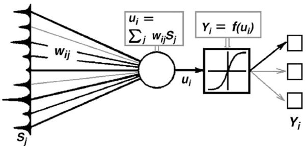
Structure of a neural network.

$$y_i=f({\mathrm{\sum }}_j{w}_{ij}{S}_j)$$ (5)

with the symbols defined below.

Input neurons, for example a spectral intensity vector S(j) consisting of nine intensity points (peaks) and represented at the left in Fig. 1, are connected to a point marked by the open circle by matrix elements representing a weight factor for each intensity input. These matrix elements are indicated by the lines w_ij of different weights in Fig. 1. The resulting quantity u_i, known as the node response, is defined by

$$u_i={\mathrm{\sum }}_j{w}_{ij}{S}_j.$$ (6)

Since the input vectors S(j) may be quite different, u_i may vary for each input vector S(j) to be tested. Therefore, a sigmoidal response function f is applied which determines the boundaries of response for a single neuron. The response function is of the form

$$f(u)=tanh(u)orf(u)=1/(1+e^{-u}).$$ (7)

For each of the possible classifications, y_i, there will be a weight vector W with j entries. These vectors W are established during the training phase of the ANN (see below), and are responsible for the gross connection between certain spectral features, and the desired “diagnosis. The summation point and subsequent response function shown in Fig. 1 form one node; the output of a node can be the input of further nodes (hidden layers) if a multilayered net is constructed.

In the “winner-takes-all” (WTA) decision stage of the ANN, the largest element y_i determines which output is triggered. For WTA, classification depends on the highest output activation. A minimum value for the winner typically is set to 0.7, and a minimum distance to the second highest activation to 0.3. The “40–20–40” function applies a different winner decision-making algorithm; the activation of one neuron must exceed 0.6 and all other activations of additional classes must be below 0.4. If not, then the spectrum remains unclassified. A common problem with different classification methodologies is the potential of misclassification due to undesired or unexpected extrapolation. This occurs when the training and validation datasets are not comprised of all classes or the entire range of features needed for a given classification problem. In this case, any classification method, including ANNs, would not be successful for the given problem. Neuro-Developer uses a distance value derived from the training and validation dataset to determine an extrapolation problem. The allowed maximum distance of a pattern to its corresponding class is calculated and set to 100. If, during classification of a pattern by the ANN, the distance of the new pattern exceeds this distance, an extrapolation has occurred, and the pattern is unclassified.

All ANN calculations were performed utilizing the Neuro-Developer^® 2.5b (Synthon, GmbH, Heidelberg, Germany) software. A three layer feed-forward network was constructed, consisting of the input layer (the intensity vector S(ν_k)), a hidden layer, and an output layer consisting of three neurons (G1, S and G2). The best network was found after testing different layouts with varying numbers of inputs and hidden nodes. The optimum number of input nodes (30) corresponds to the number of spectral data points with the highest covariance. This number may appear small, given that the input vector contains 450 intensity data points. However, given the inherent bandwidth of IR spectra of cells, and the smoothing/derivative window utilized (typically 11 to 13 points), the choice of 30 intensity points certainly appears reasonable.

For network learning, an iterative resilient back propagation (Rprop) procedure was applied. In the Rprop procedure, the first weight change update value, Δ₀, was set to 0.1, and the maximum range of update, Δ_max, to 50. ANNs can be “over-trained” to the level of incorporating features that are particular to the spectra of the cells in the training sample, rather than typical characteristics of the spectral classes they represent. For this reason, independent samples must be used to check that the net is properly classifying the cellular spectra. Thus, the 457-spectral data pool was split into training, validation and test blocks, each containing 60%, 20% and 20% of the total data pool, respectively. The software’s internal algorithm was used for testing different layouts, as well as varying the numbers of input and hidden layers. This was the case for both the top-level and sub-level net optimization (see below). The training process was stopped when the error of the validation data set reached the minimum. The best network was chosen on the basis of having the lowest validation and training data set errors. Subsequently, various single-cell IR spectra were used to test the trained ANN and perform the classification.

3. Results and discussion

After staining for cyclin E (red fluorescence), cyclin B1 (yellow fluorescence), and incorporated BrdU (green fluorescence), the fluorescence images of the cell pairs were matched with the visible images collected during the IR micro-spectroscopy. The reason for analyzing cell pairs only is the fact that all cells that survived the mitotic shake-off will appear as two new daughter cells shortly (within 1 h) after reseeding them onto the slides. Fig. 2 shows the typical staining pattern for each of the three cell populations (G1, S and G2). Positive red staining for cyclin E indicates that the cells were in the G1 phase [9] at the time of fixation. Cyclin E reaches its maximum concentration at the end of G1, and is quickly degraded during the early S phase [10].

Fig. 2.

Identifying cell cycle populations using immunohistochemical staining. Columns from left to right: Fluorescence image of cell pair, cell-cycle phase assignment, staining for cyclin E, BrdU and cyclin B1. Top row: G1-phase population. Middle row: S-phase population. Bottom row: G2-phase population.

Since the thymidine analog BrdU is integrated into nuclear DNA only during DNA synthesis during the S-phase, the positive green fluorescence staining for BrdU indicates that the cell was actively synthesizing DNA at the time of BrdU incubation. Cells that exhibit a double-staining positive for both incorporated BrdU and cyclin E are in the early stage of the S phase when they were fixed, [9] typically 6–8 h after mitotic shake-off.

Cells that exhibit green fluorescence staining only were actively synthesizing DNA at the time of fixation, but no longer contained enough cyclin E for detection. These cells were assigned to the mid-late S-phase population, found typically 11–15 h after mitotic shake-off. As indicated in Fig. 2, we grouped the cyclin E-positive/BrdU positive (early S phase) and the cyclin E-negative/BrdU-positive cells (mid-late S phase) together into the S population.

The final group exhibited only positive yellow fluorescence staining for cyclin B1, indicating that the cells contained enough cyclin B1 for detection, had completed DNA synthesis before the BrdU incubation period and had yet to enter G1 phase. These cells were assigned to the G2 phase [9]. Cyclin B1 moves into or near the nucleus toward the end of the G2 phase and reaches its maximum concentration at the G2/M phase junction, after about 18–20 h. Cyclin B1 is degraded during the M phase [11]. A representative example of the staining pattern observed for each of the populations is displayed in Fig. 2. The blue hues result from counterstaining with 4′,6-diamidino-2-phenyindole dihydrochloride (DAPI) to visualize the location of the nucleus.

For the IR spectra of HeLa cells, the differences at the various time points of the cell cycle manifest themselves mostly in changes of the amide I and II bands, and to a lesser extent, the DNA bands regions at 1090 and 1235 cm⁻¹. These changes are more evident in the second derivative spectra, shown in Fig. 3. There is a large (~10 cm⁻¹) shift in the amide I peak position, accompanied by a shift in an amide I shoulder as the cells progress through the G1, S and G2 phases, indicative of changes in protein structures [12,13] found in the nucleus at different time points [14,15]. Similar frequency shifts are observed in the amide II vibrations at 1538, 1540 and 1543 cm⁻¹ for the G1, S and G2 phases, respectively. Furthermore, the amide II peak shows a low frequency shoulder at about 1500 cm⁻¹, that is barely evident in the absorption spectra but becomes more prominent between G1, S and G2 phase. Finally, the peak at phosphodiester peak at 1238 cm⁻¹ is observed strongly in the average second derivative spectra of all populations.

Fig. 3.

Average second derivative spectra collected from each of the identified populations: G1 phase (top), S phase (center) and G2 phase (bottom). The vertical lines at 1650 and 1538 cm⁻¹ indicate the amide I and amide II peak shifts, respectively.

The spectral differences in the DNA peaks (at 1090 and 1235 cm⁻¹) are relatively small for HeLa cells, and certainly much smaller than the changes originally reported by us for leukemia cells [2]. The larger spectral changes observed for the leukemia cells may have been due to the fact that the much larger nucleus-to-cytoplasm ratio in the leukemia cells accounts for a much stronger contribution to the spectra than in epithelial cells. Furthermore, the spectral heterogeneity observed for all cultured and harvested cells was not understood at that time, and may have contributed to the observed changes.

In order to emphasize the heterogeneity of the observed spectra (particularly for the S-phase), we display in Fig. 4 variability plots, consisting of the average population plot minus the average difference for the three groups of spectra (G1, S, and G2). Whereas the spectra of the two gap phases, G1 and G2, show a relatively small variability from the average in the populations, the S-phase spectra exhibit variations nearly an order of magnitude larger than that seen in the gap phase (G1 or G2) spectra. This heterogeneity amongst the population occurs both in the spectral features of protein (amide I and II) and in those of DNA (1090 and 1235 cm⁻¹) among the spectra of cells of similar biochemical age. Such a spectral heterogeneity will make the visual inspection of individual spectra nearly impossible, and requires the use of methods of multivariate analysis for a meaningful interpretation.

Fig. 4.

Variation in FTIR-MSP over each of the cell populations. The average variation from the average second derivative spectrum of the population for each of the three populations: G1 phase (red), S phase (green) and G2 phase (blue), plotted vs. a FTIR-MSP absorption spectrum of a single cell (pink).

This is demonstrated in Fig. 5, where scores plots of cellular populations are presented. Panel A shows a separation between G1 and G2 stages, indicating that there are distinct spectral differences between these groups. These PCA results were carried out for the amide I region of the spectra (for the region 1598–1702 cm⁻¹). The amide II region shows similar results, but the separation becomes less pronounced when the entire spectral range of 800–1800 cm⁻¹ is used. This result confirms the conclusions drawn from Fig. 3 that there are systematic variations in the amide I and II vibrations between G1 and G2 stages. This result is not too surprising, considering that in G1, the proteins for DNA replication are synthesized, whereas in G2, proteins for mitosis are synthesized.

Fig. 5.

PCA results of the amide I region (ca. 1600–1700 cm⁻¹). Panel A: scores plot of G1- and G2-phase populations. Panel B: scores plot of G1-, S- and G2-phase populations.

However, the S-phase spectra do not form a distinct cluster, but span the entire PC3/PC2 space, with much larger variance than the G1/G2 cells. This is shown in Panel B of Fig. 5. Thus, we conclude that the heterogeneity of the S-phase spectra is large, and S-phase spectra cannot easily be separated from G1 and G2 phase spectra based on the amide I/II band profiles.

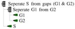
PCA results indicate that sufficient spectral differences exist between G1 and G2-phase cells to discriminate them with a supervised discriminant algorithm, such as a trained ANN. Due to the heterogeneity of the spectra of the S-phase, separating of the three classes (G1, S and G2) using a single-level ANN was not successful, even after varying the number of input neurons, hidden layers and output neurons. The G1 and G2 classes were correctly identified, but the S-phase spectra were misclassified. To remedy this, a hierarchical ANN topology was employed. In this topology, S-phase spectra are first separated from the gap-phase spectra (G1/G2). This was accomplished using a network that utilizes intensity points determined by a covariance-based feature selection, shown in Fig. 6 (black bars). This figure shows the wavenumber ranges of greatest importance for the correct separation of these cell populations by their spectra. The black bars indicate the wave-number range of highest of importance in separating the S-phase population from the non-S-phase population of cell spectra, with the height of the bar indicating the relative importance of that wavenumber to the correct separation via that subnet. The gray bars are placed at the wavenumber of importance in separating the G1-phase cell spectra from the G2-phase cell spectra (Table 1).

Fig. 6.

Separating the gap-phase pool from the S-phase pool (black) and separating the G1-phase pool from the G2-phase pool (grey), covariant importance vs. wavenumber for correct class identification.

Table 1.

Results of ANN separation of G1, S and G2 classes of spectra

Sensitivity	99%
Specificity	96%
Accuracy	97.5%

Subsequently, the gap-phase pool of spectra was separated into G1- and G2-phase spectra. The intensity points used for this classification are given by the gray bars in Fig. 6. This hierarchical network classified the three populations of the test set, consisting of about 90 spectra, correctly with a sensitivity of 99%, a specificity of 96% and an accuracy of 97.5%. Rather than utilizing the narrow frequency range employed for PCA, the network analysis was allowed to select spectral features from the entire spectral range (800–1800 cm⁻¹). Therefore, the spectral features used for classification do not necessarily occur in the spectral regions expected from visual inspection.

Although the concept of using supervised algorithms, such as ANNs, for classification of spectral data of cells without knowledge of the “biochemical cause” appears perilous, previous studies using ANN for classification of normal and bovine spongiform encephalopathy-infected (BSE) bovine plasma samples have proven extremely successful [8]. Furthermore, ANN-based analysis of IR spectra to elucidate drug action on cultured cells revealed spectral patterns diagnostic for a given mode of action of a drug [10]. In both cases, the spectral changes were too small to be detected or interpreted by visual inspection. Yet, the occurrence of minute spectral differences in hundreds of spectra allow for their diagnostic use.

The main reason why ANN algorithms fail to correctly classify all the spectra is that the Rprop algorithm is designed to deal with data comprised of Gaussian distributions. Nonetheless, it is very robust in classification problems. With the advance of more spectroscopically oriented statistical software, the failures could be overcome by applying ANNs based on the radial basis function models, and error functions more attuned for these classifications problems, such as cross-entropy methods.

4. Conclusions

We have shown that there exist small spectral differences between the infrared spectra of epithelial cells in G1 and G2 stages. These differences are sufficient for a straightforward classification by spectral methods, although the spectra of these two phases are very similar, as reported earlier [7]. Spectra of cells in the S-phase, however, are much more different to classify, since they exhibit large heterogeneity. Although cells exhibit immunohistochemical markers indicative of DNA synthesis, their spectra may be very different from, or very similar to the spectra of the gap phase (G1/G2) cells.

References

- 1.Lasch P, Chiriboga L, Yee H, Diem M. Infrared spectroscopy of human cells and tissue: detection of disease. Technol Cancer Res Treat. 2002;1:1–7. doi: 10.1177/153303460200100101. [DOI] [PubMed] [Google Scholar]
- 2.Boydston-White S, Gopen T, Houser S, Bargonetti J, Diem M. Infrared spectroscopy of human tissue. V. Infrared spectroscopic studies of myeloid leukemia (ML-1) cells at different phases of the cell cycle. Biospectroscopy. 1999;5:219–227. doi: 10.1002/(SICI)1520-6343(1999)5:4<219::AID-BSPY2>3.0.CO;2-O. [DOI] [PubMed] [Google Scholar]
- 3.Miljkovic M, Romeo M, Matthaeus C, Diem M. Infrared microspectroscopy of individual human cervical cancer (HeLa) cells suspended in growth medium. Biopolymers. 2004;74:172–175. doi: 10.1002/bip.20066. [DOI] [PMC free article] [PubMed] [Google Scholar]
- 4.Romeo M, Mohlenhoff B, Diem M. Infrared micro-spectroscopy of human cells: causes for spectral variance of oral mucosa (Buccal) cells. Vibr Spectrosc. doi: 10.1016/j.vibspec.2006.04.009. in press. [DOI] [PMC free article] [PubMed] [Google Scholar]
- 5.Romeo M, Mohlenhoff B, Jennings M, Diem M. Infrared micro-spectroscopic studies of epithelial cells. Biochim Biophys Acta. 2006;1758:915–922. doi: 10.1016/j.bbamem.2006.05.010. [DOI] [PMC free article] [PubMed] [Google Scholar]
- 6.Matthäus C, Boydston-White S, Miljkoviæ M, Romeo M, Diem M. Raman and infrared micro-spectral imaging of mitotic cells. Appl Spectrosc. 2006;60:1–8. doi: 10.1366/000370206775382758. [DOI] [PMC free article] [PubMed] [Google Scholar]
- 7.Boydston-White S, Chernenko T, Regina A, Miljkoviæ M, Matthäus C, Diem M. Microspectroscopy of single proliferating HeLa cells. Vibr Spectrosc. 2005:169–177. [Google Scholar]
- 8.Schmitt J, Beekes M, Brauer A, Udelhoven T, Lasch P, Naumann D. Identification of scrapie infection from blood serum by Fourier transform infrared spectroscopy. Anal Chem. 2002;74:3865–3868. doi: 10.1021/ac015688s. [DOI] [PubMed] [Google Scholar]
- 9.Koff A, Cross F, Fisher A, Schumacher J, Leguellec K, Philippe M, Roberts JM. Human cyclin E, a new cyclin that interacts with two members of the CDC2 gene family. Cell. 1991;66:1217–1228. doi: 10.1016/0092-8674(91)90044-y. [DOI] [PubMed] [Google Scholar]
- 10.Scott IS, Morris LS, Bird K, Davies RJ, Vowler SL, Rushbrook SM, Marshall AE, Laskey RA, Miller R, Arends MJ, Coleman N. A novel immunohistochemical method to estimate cell-cycle phase distribution in archival tissue: implications for the prediction of outcome in colorectal cancer. J Pathol. 2003;201:187–197. doi: 10.1002/path.1444. [DOI] [PubMed] [Google Scholar]
- 11.Scott IS, Heath TM, Morris LS, Rushbrook SM, Bird K, Vowler SL, Arends MJ, Coleman N. A novel immunohistochemical method for estimating cell cycle phase distribution in ovarian serous neoplasms: implications for the histopathological assessment of paraffin-embedded specimens. Br J Cancer. 2004;90:1583–1590. doi: 10.1038/sj.bjc.6601660. [DOI] [PMC free article] [PubMed] [Google Scholar]
- 12.Choo LP, Jackson M, Mantsch HH. Conformation and self-association of the peptide hormone substance P: Fourier-transform infrared spectroscopic study. Biochem J. 1994;301(Pt 3):667–670. doi: 10.1042/bj3010667. [DOI] [PMC free article] [PubMed] [Google Scholar]
- 13.Jackson M, Mantsch HH. The use and misuse of FTIR spectroscopy in the determination of protein structure. Crit Rev Biochem Mol Biol. 1995;30:95–120. doi: 10.3109/10409239509085140. [DOI] [PubMed] [Google Scholar]
- 14.Mueller GC. Biochemical events in the animal cell cycle. Fed Proc. 1969;28:1780–1789. [PubMed] [Google Scholar]
- 15.Van Hooser A, Goodrich DW, Allis CD, Brinkley BR, Mancini MA. Histone H3 phosphorylation is required for the initiation, but not maintenance, of mammalian chromosome condensation. J Cell Sci. 1998;111(Pt 23):3497–3506. doi: 10.1242/jcs.111.23.3497. [DOI] [PubMed] [Google Scholar]