OPTIMIZING MEASUREMENT OF THE ELECTRICAL ANISOTROPY OF MUSCLE

Abstract

Skeletal muscle is electrically anisotropic, with applied high-frequency electrical current flowing more easily along than across muscle fibers. As an early step in harnessing this characteristic for clinical use, we studied approaches for maximizing the measured anisotropy by varying electrode size and applied current frequency in the tibialis anterior of 10 normal subjects. The results were compared to those from two patients with amyotrophic lateral sclerosis (ALS). Current was applied percutaneously, first parallel and then perpendicular to the major fiber direction of the muscle at frequencies ranging from 20 kHz to 1 MHz, using a fixed voltage–electrode length and varying the current–electrode length. The measured anisotropy was most pronounced using the longest length current electrodes and with a 125-kHz applied frequency for the major outcome parameter phase. In addition, the two ALS patients showed very distinct anisotropic patterns. These results support the belief that, with the appropriate measurement technique, non-invasive assessment of electrical anisotropy of muscle may have useful clinical application.

Electrical impedance myography (EIM) refers to a set of impedance-measuring techniques for the assessment of neuromuscular disease.^6,8,10 The underlying premise of EIM is that the pathologic alterations that occur in neuromuscular disease states, including neurogenic (e.g., amyotrophic lateral sclerosis) and myopathic (e.g., muscular dystrophy or inflammatory myositis) disorders, produce reproducible disruptions in normal impedance characteristics of muscle. Work to date using our most basic approach, termed linear EIM, has demonstrated the potential value of EIM in a variety of these clinical contexts.^4,7,11

One property of skeletal muscle that we have not yet taken advantage of in the development of EIM is its electrical anisotropy—the property of applied electrical current flowing more readily along muscle fibers than across them.^1,2,5 Because neuromuscular diseases produce substantial pathological changes, including grouped atrophy, muscle fiber disorganization, and fatty replacement, the anisotropic pattern of the muscle is likely to be highly disturbed in these settings. However, the measurement of anisotropy requires a substantially different approach than our “standard” linear EIM technique in that the current must be applied in relative close proximity to the voltage-measuring electrodes such that the flow of current can be accurately oriented orthogonal to the axis of the voltage electrodes.¹ This requirement introduces new complexities, such as uncertainties in electrical current flow and distribution within the skin–subcutaneous fat layer and the possibility that small inconsistencies in electrode position and application will lead to large errors in measurement. Moreover, a minimum of two sets of measurements are required, with current being applied parallel (longitudinally) and perpendicular (transversely) to the major muscle fiber direction, so that an anisotropy ratio (transverse/longitudinal) can be calculated.

In this study, we assessed the anisotropic characteristics of normal muscle and its dependence on the frequency of applied current and relative size of the current-injecting and voltage-measuring electrodes with the aim of optimizing our measurement parameters for future clinical use. We also studied two subjects with amyotrophic lateral sclerosis (ALS) to provide some early clinical context as to what these measurements may have to offer in terms of disease assessment.

METHODS

Subjects

Ten normal healthy subjects (7 men and 3 women, mean age 41 years, range 20–72 years) participated in this study. Subjects had no history of neuromuscular disease, denied radicular symptoms, and had normal strength and bulk of tibialis anterior. In addition, two subjects meeting El Escorial Criteria for definite ALS, a man aged 71 years and a woman aged 75 years, were studied. The man still had full strength in the tibialis anterior, whereas the woman had not even a flicker of contraction on manual muscle testing. The study was approved by our institutional review board, and all participants signed an approved informed consent form.

EIM Measurement Equipment

Impedance measurements were made using a wide-band lock-in amplifier (Signal Recovery Model 7280; Advanced Measurement Technology, Inc., Oak Ridge, Tennessee) that supplied current at a constant voltage of 1 V at a variety of frequencies from 20 kHz to 1 MHz and was configured with a very-low-capacitance active probe (Model P6243; Tektronix, Beaverton, Oregon), as described previously.⁴

Signals from the pair of voltage electrodes (described in what follows) were returned to the impedance instrument, which converted them into analog signals proportional to the resistance (R) and the reactance (X). The resulting data were digitized and stored in a standard computer (Pavilion a250n; Hewlett Packard, Palo Alto, California) through which additional data analysis was performed, including calculation of phase (θ), the main outcome measure used in our previous studies.

Electrode Placement and Measurement

We chose to study only the tibialis anterior muscle, given its relatively straightforward geometry and the lack of excess subcutaneous tissue overlying the muscle in most individuals. The electrodes used were 0.55-cm-wide × 9.0-cm-long adhesive Ag–AgCl strips (part number 019-766400; Viasys Healthcare/Nicolet Biomedical, Madison, Wisconsin). For all voltage measurements, the electrodes were fixed to a size of 2.25 cm. This size was chosen for the practical reason that it would be just small enough to fit over the average-sized adult tibialis anterior without overlapping adjacent muscles but was not unnecessarily small so as to avoid artifacts produced by poor electrode contact. For the current electrodes, we chose three different lengths to evaluate: full-length (9 cm), half-length (4.5 cm), and one-quarter length (2.25 cm).

The major muscle fiber direction of tibialis anterior was identified by drawing a line from a point just medial to the fibular head to a point just lateral to the medial malleolus. A point approximately one-third down from the proximal site was chosen as the center of the testing area and the lines were placed with an indelible marker to assist with accurate electrode placement at 0° and 90° relative to the presumed major muscle fiber direction. The four electrodes were then placed perpendicular to the muscle fiber direction 2.5 cm apart, such that current flow was parallel to the muscle fibers (Fig. 1). After measurements were made across the entire frequency range, the electrodes were then removed, and fresh ones placed using the same interelectrode distances, but now at 90° (so that current flow was perpendicular to the muscle fibers). The procedure was then repeated for the three different-sized current electrodes studied. Fresh electrodes were used for each measurement.

FIGURE 1.

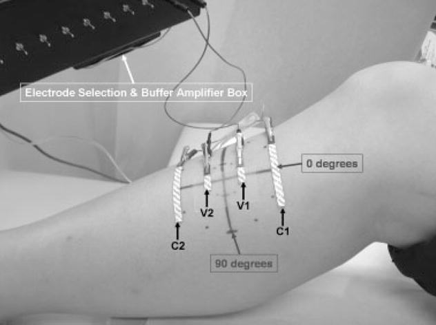
Experimental arrangement for obtaining EIM measurements at 0° on tibialis anterior. For 90° measurements, the entire array is rotated 90°, with the electrodes being kept the same distance apart.

Data Analysis

For each measurement, the resistance (R) and reactance (X) were measured and the phase (θ) calculated using the relationship θ = arctan (X/R). The anisotropy ratio (AR) was defined as the transverse/longitudinal measurement for each of the variables (X, R, and θ). X, R, and θ vs. applied frequency plots were generated.

RESULTS

Figure 2 shows the mean raw R, X, and θ plots (± standard deviation) for all 10 subjects at both 0° and 90° vs. log (frequency), using the longest current electrodes. As can be seen, X tended to be maximal, reaching a mean value of approximately 5.50 Ω near 30 – 40 kHz (37 kHz) when current flow was longitudinal to the fibers (0°), but shifted to higher frequencies (approximately 50 kHz), reaching a maximum of about 9.72 Ω on average when measured in the transverse configuration (90°). Similarly, phase was maximal near 80 kHz in the longitudinal direction, reaching a mean of about 17.0° and shifted toward a maximum at frequencies of greater than 100 kHz (125 kHz) in the transverse direction, reaching a mean of about 27.0°. In both cases, R decreased with increasing frequency, although the slope of that decrease was greater in the transverse direction.

FIGURE 2.

Mean (± standard deviation, represented by dotted lines) resistance (R), reactance (X), and phase (θ) measurements at 0° and 90° vs. log (frequency), for all 10 normal subjects.

Figure 3 shows the relationship between the measured anisotropy for R, X, and θ by incorporating the three different electrode size configurations, comparing data averaged across all 10 normal subjects. As can be seen, the maximal anisotropy for all three parameters was obtained using the longest current electrodes, although that dependence was subtler for R (and actually reversed at high frequencies). For X, anisotropy reached a maximum at approximately 80 kHz with the shortest current electrodes, and increased to about 100 kHz with the longest. For phase, the anisotropy reached a maximum at close to 150 kHz using the shortest current electrodes and increased to about 300 kHz for the longest electrodes. On an individual basis, maximal anisotropy ratios for both X and θ ranged between 1.55 and 2.26 using the longest current electrodes.

FIGURE 3.

Electrode sizes and effect on anisotropy, showing the average data for all 10 subjects. Resistance, reactance, and phase are plotted against log (frequency) for three different lengths of the current electrodes described. The greatest anisotropy is obtained with the longest current electrodes. Standard deviations are omitted for the sake of clarity.

Figure 4 provides the same anisotropy ratio data from Figure 3 using just the longest electrode length, now plotted along with the standard deviation at all frequencies, and with the data from the two ALS patients. As can be seen, the data from the two ALS patients are quite distinct from the normal subjects and also distinct from one another, with the patient with advanced disease showing a relative loss in the measured anisotropy (most clearly seen in the reactance) and the early case showing an increase.

FIGURE 4.

Mean (± standard deviation, represented by dotted lines) anisotropy ratio using the longest length electrode data for the 10 normal subjects (filled circles) with comparison to the data from the two ALS patients (squares and triangles).

DISCUSSION

These results substantially extend earlier studies^1–3,5 that first demonstrated that muscle electrical anisotropy is readily detectable. Indeed, the previous studies were limited, focusing on a small frequency range and reported results only for resistance or resistivity. Only one study evaluated the effects of reactance.³ We recently also studied the anisotropy of current flow in beef, in which we identified a considerably more prominent anisotropy ratio in reactance than in resistance.¹² These earlier studies did not seek to identify frequencies of maximal anisotropy and used technical approaches that could not be easily adaptable to assessment of single muscles. Here we have shown that the measured anisotropy is highly dependent upon both the frequency of the applied current and the electrode size configurations utilized. Moreover, the data support that, at least for tibialis anterior, these dependences are highly consistent across individuals. Finally, data from the two ALS patients suggest that disease states substantially impact this property of muscle. Why these two patients had such divergent changes, however, is unclear. One possibility is that group atrophy and reinnervation in early neurogenic disease produces elevations in anisotropy, whereas advanced disease and near-complete atrophy of all muscle fibers, with associated fatty infiltration of tissue, leads to a loss of anisotropy.

Unlike standard electrophysiologic approaches to assessing muscle, EIM relies upon the application of high-frequency electrical current, so no action potentials within the muscle are generated. Indeed, the inherent electrical anisotropy of muscle can be best understood by modeling skeletal muscle as a complex network of resistors and capacitors. The resistors reflect current flow through the intra- and extracellular fluids and the capacitors represent the cell membranes’ lipid bilayers. Current directed perpendicular to the muscle fibers needs to pass through many more myocytes than current flow parallel to the muscle fibers, leading to a much stronger capacitive effect and the observed prominent anisotropy in reactance. An analogous argument holds true with the measured resistance. In contrast to earlier studies^2,5,12 that identified substantially stronger anisotropy (e.g., a ratio of 15.3 in resistivity in the study by Rush et al.⁵), we identified relatively weak anisotropy in both resistance and reactance, with the anisotropy ratio reaching no more than about 2.0 in normal subjects. One reason for this is likely due to the fact that we applied current on the surface of the tissue through the skin and subcutaneous fat, whereas in the earlier studies, current was applied directly across the excised muscle. Indeed, our own work with beef gave considerably lower values than those studies (e.g., a ratio of 4.5 for phase), likely because current there was also applied on the surface and not across the tissue, although no subcutaneous tissues or skin were present. Finally, the boundary conditions (e.g., the shape of the lower leg) also likely impacted our data, further reducing the observed ratio.

The present results also show that the greatest anisotropy was obtained with longer current injection electrodes (Fig. 3). The reason for this likely relates to current distribution effects. With smaller current electrodes, the current tends to fan out.⁹ Thus, only part of the current will flow parallel to a line joining the mid-points of the voltage electrodes, reducing the apparent anisotropy of the tissue. Using long current injecting electrodes in relation to the voltage electrodes can help assure that the current lines are mainly parallel in the voltage-measuring region.

The explanation underlying the specific anisotropic dependences of R, X, and phase on the applied frequency is uncertain. The data clearly support the belief that maximal anisotropy occurs at greater than 125 kHz (for phase) and not at 50 kHz, which is where phase is usually measured when performing single-frequency measurements with current flow parallel to the muscle fibers. This is a somewhat unexpected result and suggests that, in refining approaches for the measurement of anisotropy for clinical use, it will be critical to focus on frequencies of current application higher than is standard.

The voltage electrode size was selected to be 2.25 cm based on practical necessities, because our goal was to make sure the array fit easily over the tibialis anterior, regardless of the direction it was being placed. Assuring that the voltage electrodes fit within the boundaries of the muscle is critical to the accurate measurement of anisotropy in a given muscle. In fact, it is possible that even a smaller-size voltage electrode (e.g., approximately 1.0 cm) might be preferable, but decreasing electrode size may lead to increasing noise from the electrode–skin interface. There is a less obvious need to restrict the size of the current electrodes, although it is possible that variations in the geometry and fiber direction of the underlying muscle between each of the voltage and current electrodes could impact the measured anisotropy to a small extent.

There are several technical and theoretical issues that also deserve further discussion. First, most muscles are not flat. The bulbous nature of a muscle may create differences in the amount of tissue that the current is traversing, thus contributing a morphologic effect to the measured anisotropy. Tibialis anterior was chosen, in fact, because it is relatively flat, and it is likely that most of the anisotropy measured herein represents a true effect of the muscle fiber geometry itself rather than a more non-specific shape effect. Another question that remains concerns the interelectrode distances. We chose the distance of 2.5 cm between voltage and current electrodes because it was a convenient length and would fit the muscle studied; this distance has also provided consistent data in earlier studies. The optimal interelectrode distance to use will likely depend on details of the skin–subcutaneous fat layer thickness. With increasing adipose tissue, a greater interelectrode distance may be required to effectively measure the anisotropy. Thus, a separate dedicated study assessing the relationship between interelectrode distance, skin–fat layer thickness, and the measured anisotropy will also be useful. Finally, no muscle has perfectly parallel muscle fibers, and thus intersubject variability and the structure of the specific muscle chosen for study will also substantially impact the measured anisotropy. For tibialis anterior, it is important that measurements be made toward the midpoint of the muscle because the fibers converge toward its proximal and distal ends.

Two other factors may also confound the data collection. As noted above, the skin–subcutaneous fat thickness impacts the measurements. As skin thickness increases, it is more likely that the current will fan out prior to reaching the muscle. This may have the effect of reducing the measured anisotropy and provides one explanation as to why the anisotropy is so much lower here than that measured on bare muscle¹² using the same basic experimental approach. One final concern is how deeply the electrical current actually penetrates the tissue. Ideally, the electrodes can be kept far enough apart so that current can penetrate effectively into the muscle, but not so far so as to lose selectivity of the individual muscles. However, it may be possible that electrode dimensions can be varied in an attempt to assess deeper muscles, as has been previously suggested.¹

The rationale for pursuing this work has been to help establish technical parameters that will be maximally sensitive to the variations in anisotropy that occur in diseased states of muscle. Now that we have obtained clarification on the appropriate electrode sizes and frequencies to use, the next step will be to perform dedicated measurements in patients with a variety of neuromuscular diseases to determine how different disease types (e.g., myopathy vs. neurogenic disease) and the acuity/chronicity of the disorder and its severity impact the measured anisotropy.

Abbreviations

ALS

amyotrophic lateral sclerosis

AR

anisotropy ratio

EIM

electrical impedance myography

References

- 1.Aaron R, Huang M, Shiffman CA. Anisotropy of human muscle via non-invasive impedance measurements. Phys Med Biol. 1997;42:1245–1262. doi: 10.1088/0031-9155/42/7/002. [DOI] [PubMed] [Google Scholar]
- 2.Burger HC, van Dongen R. Specific electrical resistance of body tissues. Phys Med Biol. 1961;5:431–447. doi: 10.1088/0031-9155/5/4/304. [DOI] [PubMed] [Google Scholar]
- 3.Epstein BR, Foster KR. Anisotropy in the dielectric properties of skeletal muscle. Med Biol Eng Comput. 1983;21:51–55. doi: 10.1007/BF02446406. [DOI] [PubMed] [Google Scholar]
- 4.Esper GJ, Shiffman CA, Aaron R, Lee KS, Rutkove SB. Assessing neuromuscular disease with multifrequency electrical impedance myography. Muscle Nerve. 2006;34:595–602. doi: 10.1002/mus.20626. [DOI] [PubMed] [Google Scholar]
- 5.Rush S, Abildskov JA, McFee R. Resistivity of body tissues at low frequencies. Circ Res. 1963;12:40–50. doi: 10.1161/01.res.12.1.40. [DOI] [PubMed] [Google Scholar]
- 6.Rutkove SB, Aaron R, Shiffman CA. Localized bioimpedance analysis in the evaluation of neuromuscular disease. Muscle Nerve. 2002;25:390–397. doi: 10.1002/mus.10048. [DOI] [PubMed] [Google Scholar]
- 7.Rutkove SB, Esper GJ, Lee KS, Aaron R, Shiffman CA. Electrical impedance myography in the detection of radiculopathy. Muscle Nerve. 2005;32:335–341. doi: 10.1002/mus.20377. [DOI] [PubMed] [Google Scholar]
- 8.Rutkove SB, Lee KS, Shiffman CA, Aaron R. Test–retest reproducibility of 50 kHz linear-electrical impedance myography. Clin Neurophysiol. 2006;117:1244–1248. doi: 10.1016/j.clinph.2005.12.029. [DOI] [PubMed] [Google Scholar]
- 9.Shiffman CA, Aaron R. Angular dependence of resistance in non-invasive electrical measurements of human muscle: the tensor model. Phys Med Biol. 1998;43:1317–1323. doi: 10.1088/0031-9155/43/5/019. [DOI] [PubMed] [Google Scholar]
- 10.Shiffman CA, Aaron R, Amoss V, Therrien J, Coomler K. Resistivity and phase in localized BIA. Phys Med Biol. 1999;44:2409–2429. doi: 10.1088/0031-9155/44/10/304. [DOI] [PubMed] [Google Scholar]
- 11.Tarulli A, Esper GJ, Lee KS, Aaron R, Shiffman CA, Rutkove SB. Electrical impedance myography in the bedside assessment of inflammatory myopathy. Neurology. 2005;65:451–452. doi: 10.1212/01.wnl.0000172338.95064.cb. [DOI] [PubMed] [Google Scholar]
- 12.Tarulli AW, Chin AB, Partida RA, Rutkove SB. Electrical impedance in bovine skeletal muscle as a model for the study of neuromuscular disease. Physiol Meas. 2006;27:1269–1279. doi: 10.1088/0967-3334/27/12/002. [DOI] [PubMed] [Google Scholar]