New metrics for comparing and assessing discrepancies between RNA 3D structures and models

Abstract

To benchmark progress made in RNA three-dimensional modeling and assess newly developed techniques, reliable and meaningful comparison metrics and associated tools are necessary. Generally, the average root-mean-square deviations (RMSDs) are quoted. However, RMSD can be misleading since errors are spread over the whole molecule and do not account for the specificity of RNA base interactions. Here, we introduce two new metrics that are particularly suitable to RNAs: the deformation index and deformation profile. The deformation index is calibrated by the interaction network fidelity, which considers base–base-stacking and base–base-pairing interactions within the target structure. The deformation profile highlights dissimilarities between structures at the nucleotide scale for both intradomain and interdomain interactions. Our results show that there is little correlation between RMSD and interaction network fidelity. The deformation profile is a tool that allows for rapid assessment of the origins of discrepancies.

INTRODUCTION

Determining RNA three-dimensional (3D) structures is key in studying RNA function (Gesteland et al. 2006). Physical methods such as X-ray crystallography and nuclear magnetic resonance (NMR) spectroscopy are the most common ways for determining RNA 3D structures at high resolution. However, these methods cannot be applied to all RNAs and RNA systems. Alternative methods include interactive modeling (Michel and Westhof 1990; Massire and Westhof 1998; Martinez et al. 2008) and conformational space searching (Das and Baker 2007; Ding et al. 2008; Parisien and Major 2008; Jonikas et al. 2009).

The development and improvement of alternative methods are highly dependent on what we learn from experimentally resolved structures. In particular, close inspection of rRNA structures revealed the presence of structural motifs that we can recognize from sequence (Lescoute et al. 2005). To assist the production of new knowledge, systematic methods to annotate RNA 3D structures (Gendron et al. 2001; Lemieux and Major 2002; Yang et al. 2003; Djelloul and Denise 2008), discover and analyze structural motifs (Huang et al. 2005; Lemieux and Major 2006; Lisi and Major 2007; Abraham et al. 2008; Xin et al. 2008), and formally represent RNA structures (Dowell and Eddy 2004; St-Onge et al. 2007) have been developed. This systematization of knowledge generation and integration in ever-improving predictive methods is typical of the post-ribosomal X-ray crystallographic era. A problem that has been largely neglected, however, is how one can measure quantitatively the improvements brought by new approaches or methods.

The classical index for comparing predictive methods is to benchmark with the average root-mean-square deviations (RMSDs) after optimal superimposition between the modeled RNA 3D structures they produce and their corresponding experimental structures. RMSDs are extremely useful, and obtaining models close to experimental structures is a noble exercise. RMSDs capture the general 3D shape of an RNA, but give little information about its base-pairing and base-stacking patterns, local deviations of the structure, intradomain deformation, or interdomain deviations. Most importantly, RMSDs spread errors over the whole molecule to obtain the best global superimposition so that it is very difficult to localize the origins of the modeling defects and thus to improve the modeling process (Yang and Honig 2000; Gendron et al. 2001; Shatsky et al. 2002). RNA molecules have specific structural features, such as a modular and hierarchical architecture of structural elements like helices, hairpins, and single-stranded loops connected by tertiary interactions. In addition, RNA bases associate in well-defined patterns of pairings that usually stack on each other. As modeling and predictive methods are getting increasingly accurate, it is now desirable that their results could be compared based on the reproducibility of these important and specific RNA structural features rather than on global average measurements.

Here, we introduce two new RNA 3D structure comparison tools: (1) an RNA 3D structure comparison index, the deformation index (DI), which evaluates and indicates the deviations between two RNA 3D structures with both RMSDs and base interactions; and (2) a deformation profile (DP), which depicts the conformation differences between two models at local, interdomain, and intradomain scales. These new tools provide quantitative measures to compare the accuracy in reproducing the base–base interaction networks of different 3D models, as well as the ability to evaluate the local and global prediction precision and quality of RNA molecules.

RESULTS

Deformation index

We define the DI as the RMSD between two optimally aligned 3D structures (general shape) divided by the base interaction network fidelity (INF). The INF is computed from the base-stacking and base-pairing annotations of both structures. For practical reasons, we use two automated annotation procedures that have been proposed recently: MC-Annotate (Gendron et al. 2001; Lemieux and Major 2002) and RNAview (Yang et al. 2003). Note that the index uses, but is not related to, the annotation programs, which are obviously prone to the quality of the reference structures.

Base-stacking and base-pairing interactions

MC-Annotate detects that two bases stack using the Gabb et al. (1996) method. The base-stacking annotation results are described using the Major and Thibault (2007) nomenclature, which indicates the relative orientation of the two bases. The relative orientation is determined by comparing the direction of the normal vectors of each base, i.e., the rotational vector obtained by a right-handed axis system defined by atoms N1 to N6 around the pyrimidine ring (Fig. 1A).

FIGURE 1.

Base-stacking and base-pairing nomenclature. (A) Normal vectors in pyrimidines and purines. Using a right-handed axis system, the normal vector in the pyrimidine (left) comes out of the paper plane (atom numbers counterclockwise), whereas it is reversed in the pyrimidine ring of the purine (atom numbers clockwise). (B) The four base-stacking types. Using the normal vectors (represented by arrows), we can distinguish three types of base stacking. If base A is below base B, the normal vector of A points to B, and both normal vectors point in the same direction (left), then base B is stacked upward of A (or symmetrically base A is stacked downward of B). If the normal vectors of A and B point toward each other (middle), then bases A and B stack inward. If the normal vectors flee each other (right), then bases A and B stack outward. (C) Base edges. Each base is divided into three edges: the Watson–Crick (W) edge is at the tip of the base and where the chemical groups involved in Watson–Crick base pairs interact; the Hoogsteen (H) edge is on the opposite side of the ribose; and the sugar (S) edge is on the side of the ribose. Here is a cis A–U Watson–Crick base pair, and we write W/W cis and represent it using the black dot. The fact that any edge in any base can interact with any other edge in a partner results in six different base–base interactions: W/W, W/H, W/S, H/H, H/S, and S/S. Since there are two possible relative orientations of the ribose according to the place formed by the two bases of a base pair, then this nomenclature describes 12 different base-pairing patterns. (D) The 12 base-pairing patterns, or types, and their associated symbols.

Two possible relative orientations in each base result in four base-stacking types: upward (>>), downward (<<), outward (<>), and inward (><) (see Fig.1B). Two vectors pointing in the same direction (upward and downward) corresponds to the base-stacking type in canonical A-RNA double helices. Upward or downward is chosen depending on which base is referred to first (i.e., A>>B means B is stacked upward of A, or A is stacked downward of B). The two other types are, respectively, inward (A><B; A or B is stacked inward of, respectively, B or A) and outward (A<>B; A or B is stacked outward of, respectively, B or A).

MC-Annotate uses an unsupervised machine-learning approach to detect H-bonds and H-bonding patterns (Lemieux and Major 2002), and RNAview uses geometrical constraints (Yang et al. 2003). Both programs describe their base-pairing annotations using the Leontis and Westhof nomenclature. Each type describes the interacting edge of the two bases. Three interacting edges are defined: the Watson–Crick edge: ● (cis), ○ (trans); the Hoogsteen edge: ■ (cis), □ (trans); and the sugar edge: ◀ (cis), ◁ (trans) (Fig. 1C; Leontis and Westhof 2001). The cis/trans notation reflects the relative orientation of the backbone according to the median of the plane formed by the two bases. In Figure 1C, the base pair is cis since the riboses are positioned on the same side of the base-pair plane. When two bases interact by the same edge, only one symbol is used. For instance, a trans X–Y Hoogsteen base pair is either written “H/H trans” or X□Y. Figure 1D lists all possible base-pairing types that are described by this nomenclature.

The DI considers the full set of interactions, i.e., base-stacking and base-pairing interactions defined by the classical two-dimensional (2D) structure (A–U and G–C Watson–Crick and G–U Wobble base pairs that form in the stems); extended 2D structures (the noncanonical base pairs, but that can be represented in the dot–bracket notation); and tertiary structure interactions, such as nonhelical stacking and long-range base pairs. Note that ∼40% of the interactions in crystallized ribosomal RNAs enter the latter category (Stombaugh et al. 2009).

Interaction network fidelity

A stacking or pairing interaction, I, involves two distinct nucleotides, N_i and N_j, i < j, to form an interaction (N_i, N_j, I), where I is one of the above base-pairing or base-stacking types. The annotation of a 3D structure produces a set, S, of such interactions. Given the two sets of interactions in two distinct RNA structures, we can then compare them using simple set theory operations.

Let S_r be the set of interactions in a reference structure (usually an experimentally resolved structure) and S_m the set of interactions of a modeled structure. The interactions found in the intersection of both sets are true positives, TP = S_r ∩ S_m. The interactions in S_m that are not present in S_r are false positives, FP = S_m\S_r. The interactions absent in S_m but present in S_r are false negatives, FN = S_r\S_m.

The Matthews correlation coefficient (MCC) is estimated by:

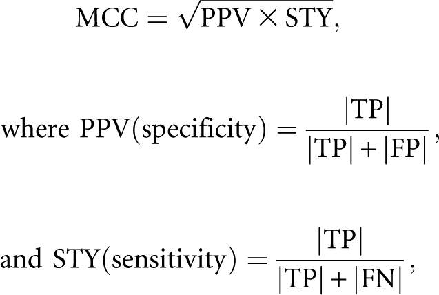(Gorodkin et al. 2001). When the model reproduces exactly the base interactions of the reference, then | FP | = | FN | = 0, | TP | > 0, and thus MCC = 1. When the model does not reproduce any of the interactions of the reference structure, then MCC = 0, since | TP | = 0.

We define the interaction network fidelity (INF) between structures A and B as the MCC, INF(A,B) = MCC(A,B). We propose a new measure of the resemblance between two structures A and B (for example, a model and its corresponding experimental structure), which is quantified by a deviation index,

Not having an INF, the DI would simply be the RMSD. However, given an INF from 0 to 1, then the RMSD between A and B could either have a large (and even infinite) DI if the two structures share no common interactions (INF = 0), or meaningful RMSD as INF approaches 1 (i.e., the majority of the interactions in A are reproduced in B).

Example: Modeling the rat 28S rRNA loop E 3D structure

Consider the crystal structure of the rat 28S rRNA loop E (PDB code 1Q9A; resolution 1.04 Å; Correll et al. 2003) shown in Figure 2A. MC-Annotate (Fig. 2B) and RNAview (Fig. 2C) were used to compute the base-pairing network of this structure. Since RNA structure annotation is subject to interpretation and small geometrical variations—for instance, MC-Annotate is stricter than RNAview—we therefore take the intersection of both programs. MC-Annotate also computes the base-stacking network (see Fig. 2D).

FIGURE 2.

The rat 28S rRNA loop E structure. (A) Stereoview of the crystal structure (PDB code 1Q9A). (Green) Adenosines, (yellow) cytosines, (violet) guanosines, (red) uracils. The thread through the phosphate atoms is shown using a cylinder. Each base ring is filled and highlighted by thick covalent bonds. The H-bonded bases of the characteristic loop E structure, here the G9-U10-A19 base triple, are linked with dotted lines. Note that U1 in this crystal structure is not paired with G27. The image was generated using Pymol. (B) Secondary structure annotated by MC-Annotate. (C) Secondary structure annotated by RNAview. (D) Stacking annotation.

To illustrate the benchmarking of RNA 3D structure modeling results, we generated loop E 3D structures using MC-Sym (Parisien and Major 2008; see Materials and Methods). We generated a decoy of 9847 3D structures, where each structure is at least at 1 Å RMSD from each other. The RMSDs (all atoms but H) between these structures and the crystal structure range from 1.6 Å to 7.8 Å, whereas the INF values range from 0.49 to 0.89 (Fig. 3). We note that for a given RMSD threshold, we have a wide range of INF values, and for a given INF threshold, we have a wide range of RMSDs. However, as RMSDs worsen, the INF values also worsen. We note an absence of population in the upper right corner (i.e., high RMSD and high INF values). The Pearson correlation coefficient between RMSD and INF values is P = 0.60 for this particular decoy.

FIGURE 3.

Distribution of (RMSD, INF) values. For each MC-Sym generated structure, the RMSD and INF values when compared with the crystal structure are plotted. The oblique line is the linear regression (P = 0.6). The horizontal line is at an INF of 0.85, and the vertical line at 2.0 Å RMSD.

For further analyses, we randomly selected three of the MC-Sym-generated structures. Structure A is located in the upper-left corner of Figure 3 and is shown in Figure 4A. This structure has good RMSDs (1.64 Å) with the crystal structure, and good INF and DI values, 0.88 and 1.86, respectively. Since RMSDs are averaged values, they do not inform about the maximum modeling error. Therefore, we also report the max RMSD(i,j) (j > i), i.e., the maximum RMSD over any sequence fragment defined by i and j; j > i. If we exclude from the analysis the dangling nucleotide U1 in the crystal structure, the fragment that has maximum RMSD with the crystal structure is C20–C21 with 1.7 Å. This is shown by the fact that C20 and C21 are base paired in the generated structures, as annotated by RNAview, but they have problematic geometries in the crystal structure, as indicated by the absence of annotation by MC-Annotate (Fig. 2B).

FIGURE 4.

Three models of the rat 28S rRNA loop E. The models are shown colored and the crystal structure in gray (PDB code 1Q9A). (Blue) Well modeled regions (RMSD < 0.5 Å), (red) badly modeled regions (RMSD > 3.0 Å). The models were optimally aligned (all atoms but H) with the crystal structure. (A) Model with a good INF (0.88; TP 29; FP 6; FN 2) and a good RMSD (1.64 Å); DI = 1.86. (B) Model with a good INF (0.88; TP 28; FP 5; FN 3), but a bad RMSD (3.76 Å); DI = 4.30. Although the geometry of the base pairs is well conserved, the thread through the phosphate atoms is shifted. (C) Model with a bad INF (0.71; TP 21; FP 7; FN 10), but a good RMSD (2.03 Å); DI = 2.85. The thread through the phosphate atoms is well superimposed, but the base-pairing geometry is wrong. Structural features that lead to a bad INF include: (D) base-stacking parameters that differ between the crystal (yellow) and model (blue) structures, such as G9, which shows a high rise in the crystal structure when compared with the model, and A19, for which a tilt can be observed between the crystal and model structures; and (E) base-pairing parameters that differ between the crystal and model structures, such as C20, which flips (propeller twist of 180°) between the crystal and model structures.

Structure A contains 29 TP, i.e., 29 of the 30 base interactions (10 base pairs and 20 base stacks) in the crystal structure. Six FP are made: (1, 2) two upward stacking between C3–U4 and C5–C6. Note that in principle these base-stacking interactions make sense since they are located in a stem. They were not detected in the crystal structure by MC-Annotate; (3) a flip of the C20 base around the glycosidic bond creates an inward stacking A19–C20; (4) as assumed in the modeling, A8–C20 now form a base pair (H/W trans); (5) the dangling nucleotide U1 in the models is base paired to G27 as a canonical W/W cis type; and (6) as assumed in the modeling, U7–C21 now form a base pair (S/H trans). Due to the C20 base flip, the upward stacking A19–C20 and C20–C21 are not reproduced, making two FN.

Structure B was selected in the upper right section of Figure 3, i.e., it has a good INF (0.88), but a bad RMSD with the crystal structure (3.76 Å). It is shown in Figure 4B. If we remove U1, the worst fragment is G2–C20 (19-nucleotides [nt] long) with 3.66 Å. This is shown in Figure 4B by a shifted backbone in almost all nucleotide positions. Structure B contains 28 of the 30 base interactions (10 base pairs and 20 base stacks) in the crystal structure. Five FP are made. They are the same as in structure A, but the upward stacking between C5–C6 is absent as in the crystal structure. The two FN due to the C20 base flip are also present in structure B. In addition, no inward base stacking is detected between G9 and G18.

Finally, structure C (Fig. 4C) was selected in the lower left region of Figure 3, i.e., bad INF (0.71), but relatively good RMSD (2.03 Å). Again, the worst fragment is G2–C20, but its RMSD is now 2 Å. What hurts the RMSD of this model is related to difficulties to reproduce the base triple and the A8–C20 base pair of the crystal structure; typical errors in RNA modeling. In our particular case, it is noteworthy that the bases in the generated base triple have a more planar geometry than those observed in the crystal structure (Fig. 4D). As for the A8–C20 base pair, its H/W trans type now makes a consensus between MC-Annotate and RNAview. Structure C contains 21 of the 30 base interactions in the crystal structure. Seven FP are made: (1–5) are the same as in structure A; but, in addition, (6) an upward stacking between A16–G17 is detected that was not detected in the crystal structure; (7) the flanking base pair of the GAGA tetraloop, which is changed to a W/H trans (S/H trans in the crystal). The three FN of structure B are also made in structure C (two are due to the C20 base flip) (Fig. 4E). In addition, four upward stackings are not detected between A11–C12, C12–G13, A14–G15, and U4–C5. The outward stacking between G13–G17 and the G9–U10 S/H cis base pair are also not detected. The tenth FN is the absence of the S/H trans G13–A16 base pair.

Deformation profile

The DP is a distance matrix representing the average distance between a predicted model (PM) and reference model (RM). The DP matrix is obtained by (1) computing all 1-nt superimposition of PM over RM and then (2) for each superimposition, computing the average distance between each base in RM and the corresponding base in PM. Let RM_i and PM_i represent the ith nucleotides of RM and PM respectively, let SUP(A_i,B_i) be the model that results from the superposition of model B over the reference model A, minimizing the RMSDs between all the atoms of the nucleotides A_i and B_i, and let AVG_DIST(A_i,B_i) be the average distance between all atoms of the nucleotides A_i and B_i. Thus, the deformation profile of PM regarding RM is defined as:

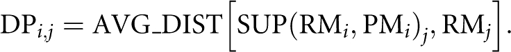Figure 5 illustrates the process of computing a DP matrix.

FIGURE 5.

Building steps of the deformation profile. (A) A predicted model (PM) will be compared with the reference model (RM). After superimposing PM over RM, minimizing the RMSD between nucleotides 2 (B) and 4 (C), the average distances between all atoms of corresponding nucleotides is calculated and recorded in DP matrix (D).

Once a pair of nucleotides (PM_i, RM_i) is superimposed, every other pair of nucleotides will be closer or farther depending on how well PM_i predicts RM_i. Those average distances are represented in the ith row of the matrix. Thus, the row average provides information about local similarity regarding the ith nucleotide. For example, an individual row with higher values than the rest of the matrix (Figs. 6, 7, represented as yellow/red rows in the DP matrices) usually means a particularly poorly predicted nucleotide. The jth column of the matrix contains the average atomic distances between the jth nucleotides of PM and RM, for each superimposition. Thus, the column average indicates how the distance between PM_j and RM_j depends on the overall prediction of all nucleotides. Finally, the main diagonal contains the average atomic distance of each nucleotide, allowing a perspective of individual nucleotide conformation similarity.

FIGURE 6.

Deformation Profile between predicted model 553 and the hammerhead ribozyme crystal structure. (A) DP matrix. Blue and pink squares inside the matrix correspond to intra- and interdomain similarity relationships, respectively. Numbers in the left top corner of each square are the average value of all positions inside the square. Color scale goes from 0 Å (white) to (but not including) 20 Å (dark green) in 10 equal steps and from 20 Å (yellow) to 80 Å (red) in five equal steps. (B) Average values of rows (green), columns (black), and main diagonal (red) of the matrix. (Shaded green regions) Helical strands. (C) 3D structure of the model. Each nucleotide is colored according to the respective row average value, from minimum (white) to maximum deformation (red) value. (D) Superimposition of the model and reference 3D structures. (E) Interaction network of the original molecule.

FIGURE 7.

Same as Figure 6 but for model 633.

An interesting property of DP is the ability to reveal similarity information at several structural scales. The rectangles corresponding to the intersection of two strands indicate the relative similarity between those strands. This way, one can easily apprehend the structural similarity at intradomain (such as between both strands of a helix or the nucleotides of a loop) and interdomain scales (such as between two helices or two loops).

It is worth noticing that values in a DP are not normalized across the whole matrix. Values close to the main diagonal tend to be smaller than values farther away. This is because nucleotide pairs closer from the superimposing pair tend to have smaller average atomic distances than those farther away. Consequently, one should only compare DP values from regions at similar distances to the main diagonal or, obviously, values from DPs of distinct models.

Example: The hammerhead ribozyme

To exemplify the deformation profile, we compared three predicted models of a hammerhead ribozyme with the reference crystal structure (PDB: 1NYI) (Dunham et al. 2003). We generated a decoy of 9999 3D structures, where each structure is at least at 1 Å RMSD from each other. The RMSDs (all atoms but H) between these structures and the crystal structure range from 2.5 Å to 15.8 Å. Selecting models from decoys is a thorny question. Here, we limited our analysis to a series of structural properties offered by the MC-Pipeline website (see Materials and Methods). We reduced the decoy by performing a five-clustering of the 10,000 models, and selecting one model per cluster that has a small volume (<25,000), a good P-Score (<−15), and to either be bipolar or coplanar (at the >0.7 level) (Laederach et al. 2007). The “thresholds” were established by comparing each structural property with RMSDs to the crystal structure (Supplemental Fig. S1). The selected models and their properties are shown in Table 1.

TABLE 1.

Structural parameter values for five models of the hammerhead ribozyme

From the modeling results, we further analyzed models 553, 633, and 2698, the resulting DPs of which are pictured in Figures 6 and 7, and Supplemental Figure S2, respectively. The models share 3.4, 12.2, and 4.9 Å RMSDs with the crystal structure, respectively. The helical regions of the models score fairly well and much better than interhelical and interloop regions (Table 2). Not surprisingly, nucleotides involved in canonical WC base pairing are better predicted than nucleotides involved in noncanonical base pairs or in loops. The 3- and 2-nt-long single-stranded regions (L1 and L3) present the worst deformation score of all short (<5-nt) contiguous regions (Supplemental Fig. S3), except for L3 in model 2698, which was particularly well predicted. The difficulty in predicting L1 and L3 also reflects in the poor prediction of the relative positions of L1 and L3. The main difference between prediction quality among the three models is due to the relative position of helix H1 with respect to the other two helices. Noticeably, the coaxial stacking of helices H2 and H3 was reasonably well predicted in all three models. While model 553 scored well in all helix–helix relative positions, models 633 and 2698 present a displacement of helix H1 regarding H2 and H3. In model 2698, helix H1 is slightly twisted, which significantly penalizes H1×H2 and, to a lesser extent, H1×H3. In model 633, helix H1 has its double-helical axis rotated by half a turn, pointing in the opposite direction of H1 in the reference molecule, which is reflected in the high values of H1×H2 and H1×H3.

TABLE 2.

Intradomain and interdomain scores for all helices, loops, helix–helix, and loop–loop combinations

DISCUSSION

So far, the field of 3D structural modeling has been driven by RMSD comparisons. In particular, GDT-TS (global distance test) is a measure that accounts for the number of atoms that are within 1, 2, 4, and 8 Å of the RMSD from a reference structure (Zemla et al. 1999; Ginalski et al. 2005). A perfect model scores 1.0. Recently, optimal GDT-TS scores of ∼0.35 for a tRNA (∼75 nt) and 0.20 for the P4–P6 domain of a group I intron (∼150 nt) have been reported (Jonikas et al. 2009). In our study, the optimal score for the hammerhead ribozyme (∼40 nt) is 0.68. However, when objectively selecting models from decoys by applying K-clustering, GDT-TS scores of 0.20, 0.06, and 0.60 are obtained, respectively. In comparison, protein structure predictions now reach GDT-TS scores as high as 0.75 on average (Zhang 2008). These results highlight the fact that there is a need for improved RNA model selection and generation methods.

RMSD-based measures might be a sufficient criterion for modeling protein structures since the backbone trace is indicative of the structure and correct positioning of the side chains (Dunbrack and Cohen 1997). However, RNA structures contain specific patterns of interacting side chains that are characteristic of folded modules and typical to each overall architecture (Lescoute and Westhof 2006). To evaluate adequately the accuracy of a predicted model, it is key to assess how well such tertiary modules and the non-Watson–Crick base pairs have been reproduced. We show that, in the context of the modeling example we used, the Pearson coefficient between RMSD and INF values (P = 0.6) presents little correlation between the two indexes. Our results further show that RMSDs do not provide information about the quality and fidelity of the base interaction network. Besides, the Pearson coefficient for structures with RMSD ≥3.0 Å (P = 0.2) is even weaker. These results point to the potential risk of using averaged values such as RMSD in evaluating the quality of RNA 3D models and, thus, the structure prediction methods that generate them. Besides, if the correlation on a small hairpin RNA example is already low, then it is expected to be even lower on larger RNAs.

Besides, the INF is less subject to variations than RMSD for an RNA under thermal motion (Grishaev et al. 2008). Intrahelical distortions include: collective atomic motion resulting in slight helix twisting that rarely affect base–base interactions (Fig. 4B), and relative atomic motion that is handled by discretizing the base–base interactions using symbolic annotation (Gendron et al. 2001; Leontis and Westhof 2001; Lemieux and Major 2002; Yang et al. 2003). Interhelical disposition from thermal motion affects the angle between helices, which greatly affects atomic distances and thus RMSD. However, such changes in general concern only a small fraction of the base–base interactions, and thus do not affect much the INF (Table 1).

In the structure prediction field, models <3 Å of RMSD from an experimental structure are considered accurate. Our results suggest extreme prudence at this particular value, since in our test case the INF value of such models can be as low as 0.7. In our example, structure C has an INF of 0.71. This structure, despite 21 TP, also had seven FP and 10 FN. If we look between 3 and 5 Å of RMSD, then INF values can be as low as 0.5; with a wider range of INF values (0.5–0.9) located at or near 4 Å of RMSD. Clearly, assessing the quality and accuracy of any given RNA 3D model needs both the RMSD and INF values.

Capturing the dissimilarity between two structures in a single value, as does RMSD, is a practical way of assessing the accuracy of predicted models. However, a single value cannot provide enough information about the shape of the actual structure and the local dissimilarities. Understanding the contribution of individual domain—nucleotides, helices, single-stranded regions—to an overall dissimilarity score demands the intervention of a human expert, which is not compatible with the analysis of dozens or hundreds of candidate models produced by automatic prediction tools. The proposed deformation profile provides a compact representation of RNA model dissimilarities from nucleotide length to intradomain scales and can be used in complement to the DI to fully assess the quality of predicted models.

Consequently, a full quantification of the comparison between two RNA 3D structures should include the overall RMSD, max RMSD(i,j), INF, as well as the DI. If only one value is to be used, then the DI is the most significant one since it reflects the overall features encoded by the RMSD calibrated by the quality of the reproduced interaction network, which is encoded by the INF value. As the size of modeled RNAs increases, the importance of using both quantifiers increases as well since the correlation between RMSD and INF values is expected to decrease. Finally, phosphate or backbone atom-only, as well as canonical base-paired region-only RMSD, should be avoided since they are not indicative of the quality of the produced models, and the field has now made sufficient progress in RNA 3D modeling and prediction methods so that all-atom models are now the gold standard.

MATERIALS AND METHODS

Generating MC-Sym decoys

To generate a decoy for the Loop E, we produced an MC-Sym script from the dot-bracket notation supported by the RNAview annotated secondary structure, “((((((((.((((..)))))))))))).” The Dot2Sym program is an MC-Tool to generate MC-Sym input scripts from dot-bracket notations (see Supplemental Information). Note that no base-pairing type information is used, and MC-Sym in such a case attempts all consistent base-pairing types.

For the hammerhead ribozyme, we also obtained a first script from Dot2Sym using the following dot-bracket input: “((((((…((((((((..))))))))(((((..))))))))))).” The script was manually edited and can be found in the provided Supplemental Information. We reduced the 10,000 structure decoys to a list of five models using the five-clustering and the following SQL query:

SELECT * FROM BKOiY0dM2m T1 INNER JOIN (SELECT MIN(PScore) AS minP, Cluster FROM BKOiY0dM2m WHERE ((Bipolar >= 0.7) OR (Coplanar >= 0.7)) and Volume <= 25000 and PScore <= -15 GROUP BY Cluster) T2 ON T1.PScore = T2.minP and T1.Cluster = T2.Cluster WHERE T1.Volume <= 25000

See the MC-Sym FAQ (http://www.major.iric.ca/MC-Sym/faq.html), commands.html page generated by MC-Sym, and the MC-Pipeline website for details (http://www.major.iric.ca/MC-Pipeline). The 3D structures were visualized and rendered using Pymol (DeLano 2002).

RMSD

RMSD values were for all-atom but H, as computed using the MC-RMSD program. MC-RMSD is part of the MC-Tools, which are available from the authors.

Deformation profile

All the data processing, PDB file manipulation, and superimposition used to compute the Deformation Profile were done in Python using Bio.PDB (http://biopython.org) and NumPy (http://numpy.scipy.org/). The script to produce DP matrices is available from the authors.

SUPPLEMENTAL MATERIAL

Supplemental material can be found at http://www.rnajournal.org.

REFERENCES

- Abraham M, Dror O, Nussinov R, Wolfson HJ. Analysis and classification of RNA tertiary structures. RNA. 2008;14:2274–2289. doi: 10.1261/rna.853208. [DOI] [PMC free article] [PubMed] [Google Scholar]
- Correll CC, Beneken J, Plantinga MJ, Lubbers M, Chan YL. The common and the distinctive features of the bulged-G motif based on a 1.04 Å resolution RNA structure. Nucleic Acids Res. 2003;31:6806–6818. doi: 10.1093/nar/gkg908. [DOI] [PMC free article] [PubMed] [Google Scholar]
- Das R, Baker D. Automated de novo prediction of native-like RNA tertiary structures. Proc Natl Acad Sci. 2007;104:14664–14669. doi: 10.1073/pnas.0703836104. [DOI] [PMC free article] [PubMed] [Google Scholar]
- DeLano WL. The PyMOL molecular graphics system. DeLano Scientific; San Carlos, CA: 2002. [Google Scholar]
- Ding F, Sharma S, Chalasani P, Demidov VV, Broude NE, Dokholyan NV. Ab initio RNA folding by discrete molecular dynamics: From structure prediction to folding mechanisms. RNA. 2008;14:1164–1173. doi: 10.1261/rna.894608. [DOI] [PMC free article] [PubMed] [Google Scholar]
- Djelloul M, Denise A. Automated motif extraction and classification in RNA tertiary structures. RNA. 2008;14:2489–2497. doi: 10.1261/rna.1061108. [DOI] [PMC free article] [PubMed] [Google Scholar]
- Dowell RD, Eddy SR. Evaluation of several lightweight stochastic context-free grammars for RNA secondary structure prediction. BMC Bioinformatics. 2004;5:71–85. doi: 10.1186/1471-2105-5-71. [DOI] [PMC free article] [PubMed] [Google Scholar]
- Dunbrack RL, Jr, Cohen FE. Bayesian statistical analysis of protein side-chain rotamer preferences. Protein Sci. 1997;6:1661–1681. doi: 10.1002/pro.5560060807. [DOI] [PMC free article] [PubMed] [Google Scholar]
- Dunham CM, Murray JB, Scott WG. A helical twist-induced conformational switch activates cleavage in the hammerhead ribozyme. J Mol Biol. 2003;332:327–336. doi: 10.1016/s0022-2836(03)00843-x. [DOI] [PubMed] [Google Scholar]
- Gabb HA, Sanghani SR, Robert CH, Prevost C. Finding and visualizing nucleic acid base stacking. J Mol Graph. 1996;14:6–11. doi: 10.1016/0263-7855(95)00086-0. 23–24. [DOI] [PubMed] [Google Scholar]
- Gendron P, Lemieux S, Major F. Quantitative analysis of nucleic acid three-dimensional structures. J Mol Biol. 2001;308:919–936. doi: 10.1006/jmbi.2001.4626. [DOI] [PubMed] [Google Scholar]
- Gesteland RF, Cech TR, Atkins JF, editors. The RNA world. CSHL Press; Cold Spring Harbor, NY: 2006. [Google Scholar]
- Ginalski K, Grishin NV, Godzik A, Rychlewski L. Practical lessons from protein structure prediction. Nucleic Acids Res. 2005;33:1874–1891. doi: 10.1093/nar/gki327. [DOI] [PMC free article] [PubMed] [Google Scholar]
- Gorodkin J, Stricklin S, Stormo G. Discovering common stem–loop motifs in unaligned RNA sequences. Nucleic Acids Res. 2001;29:2135–2144. doi: 10.1093/nar/29.10.2135. [DOI] [PMC free article] [PubMed] [Google Scholar]
- Grishaev A, Ying J, Canny MD, Pardi A, Bax A. Solution structure of tRNAVal from refinement of homology model against residual dipolar coupling and SAXS data. J Biol NMR. 2008;42:99–109. doi: 10.1007/s10858-008-9267-x. [DOI] [PMC free article] [PubMed] [Google Scholar]
- Hao MH, Rackovsky S, Liwo A, Pincus MR, Scheraga HA. Effects of compact volume and chain stiffness on the conformations of native proteins. Proc Natl Acad Sci. 1992;89:6614–6618. doi: 10.1073/pnas.89.14.6614. [DOI] [PMC free article] [PubMed] [Google Scholar]
- Huang H-C, Nagaswamy UMA, Fox GE. The application of cluster analysis in the intercomparison of loop structures in RNA. RNA. 2005;11:412–423. doi: 10.1261/rna.7104605. [DOI] [PMC free article] [PubMed] [Google Scholar]
- Jonikas MA, Radmer RJ, Laederach A, Das R, Pearlman S, Herschlag D, Altman RB. Coarse-grained modeling of large RNA molecules with knowledge-based potentials and structural filters. RNA. 2009;15:189–199. doi: 10.1261/rna.1270809. [DOI] [PMC free article] [PubMed] [Google Scholar]
- Laederach A, Chan JM, Schwartzman A, Willgohs E, Altman RB. Coplanar and coaxial orientations of RNA bases and helices. RNA. 2007;13:643–650. doi: 10.1261/rna.381407. [DOI] [PMC free article] [PubMed] [Google Scholar]
- Lemieux S, Major F. RNA canonical and noncanonical base pairing types: A recognition method and complete repertoire. Nucleic Acids Res. 2002;30:4250–4263. doi: 10.1093/nar/gkf540. [DOI] [PMC free article] [PubMed] [Google Scholar]
- Lemieux S, Major F. Automated extraction and classification of RNA tertiary structure cyclic motifs. Nucleic Acids Res. 2006;34:2340–2346. doi: 10.1093/nar/gkl120. [DOI] [PMC free article] [PubMed] [Google Scholar]
- Leontis NB, Westhof E. Geometric nomenclature and classification of RNA base pairs. RNA. 2001;7:499–512. doi: 10.1017/s1355838201002515. [DOI] [PMC free article] [PubMed] [Google Scholar]
- Lescoute A, Westhof E. The interaction networks of structured RNAs. Nucleic Acids Res. 2006;34:6587–6604. doi: 10.1093/nar/gkl963. [DOI] [PMC free article] [PubMed] [Google Scholar]
- Lescoute A, Leontis NB, Massire C, Westhof E. Recurrent structural RNA motifs, isostericity matrices, and sequence alignments. Nucleic Acids Res. 2005;33:2395–2409. doi: 10.1093/nar/gki535. [DOI] [PMC free article] [PubMed] [Google Scholar]
- Lisi V, Major F. A comparative analysis of the triloops in all high-resolution RNA structures reveals sequence structure relationships. RNA. 2007;13:1537–1545. doi: 10.1261/rna.597507. [DOI] [PMC free article] [PubMed] [Google Scholar]
- Major F, Thibault P. RNA tertiary structure prediction. In: Lengauer T, editor. Bioinformatics: From genomes to therapies. Vol. I. Wiley-VCH; Weinheim, Germany: 2007. pp. 491–539. [Google Scholar]
- Martinez HM, Maizel JV, Jr, Shapiro BA. RNA2D3D: A program for generating, viewing, and comparing three-dimensional models of RNA. J Biomol Struct Dyn. 2008;25:669–683. doi: 10.1080/07391102.2008.10531240. [DOI] [PMC free article] [PubMed] [Google Scholar]
- Massire C, Westhof E. MANIP: An interactive tool for modeling RNA. J Mol Graphics Modell. 1998;16(4–6):197–205. doi: 10.1016/s1093-3263(98)80004-1. 255–257. [DOI] [PubMed] [Google Scholar]
- Michel F, Westhof E. Modeling of the three-dimensional architecture of group I catalytic introns based on comparative sequence analysis. J Mol Biol. 1990;216:585–610. doi: 10.1016/0022-2836(90)90386-Z. [DOI] [PubMed] [Google Scholar]
- Parisien M, Major F. The MC-Fold and MC-Sym pipeline infers RNA structure from sequence data. Nature. 2008;452:51–55. doi: 10.1038/nature06684. [DOI] [PubMed] [Google Scholar]
- Shatsky M, Nussinov R, Wolfson HJ. Flexible protein alignment and hinge detection. Proteins. 2002;48:242–256. doi: 10.1002/prot.10100. [DOI] [PubMed] [Google Scholar]
- St-Onge K, Thibault P, Hamel S, Major F. Modeling RNA tertiary structure motifs by graph-grammars. Nucleic Acids Res. 2007;35:1726–1736. doi: 10.1093/nar/gkm069. [DOI] [PMC free article] [PubMed] [Google Scholar]
- Stombaugh J, Zirbel CL, Westhof E, Leontis NB. Frequency and isostericity of RNA base pairs. Nucleic Acids Res. 2009;37:2294–2312. doi: 10.1093/nar/gkp011. [DOI] [PMC free article] [PubMed] [Google Scholar]
- Xin Y, Laing C, Leontis NB, Schlick T. Annotation of tertiary interactions in RNA structures reveals variations and correlations. RNA. 2008;14:2465–2477. doi: 10.1261/rna.1249208. [DOI] [PMC free article] [PubMed] [Google Scholar]
- Yang AS, Honig B. An integrated approach to the analysis and modeling of protein sequences and structures. I. Protein structural alignment and a quantitative measure for protein structural distance. J Mol Biol. 2000;301:665–678. doi: 10.1006/jmbi.2000.3973. [DOI] [PubMed] [Google Scholar]
- Yang H, Jossinet F, Leontis N, Chen L, Westbrook J, Berman H, Westhof E. Tools for the automatic identification and classification of RNA base pairs. Nucleic Acids Res. 2003;31:3450–3460. doi: 10.1093/nar/gkg529. [DOI] [PMC free article] [PubMed] [Google Scholar]
- Zemla A, Venclovas C, Moult J, Fidelis K. Processing and analysis of CASP3 protein structure predictions. Proteins. 1999;(Suppl 3):22–29. doi: 10.1002/(sici)1097-0134(1999)37:3+<22::aid-prot5>3.3.co;2-n. [DOI] [PubMed] [Google Scholar]
- Zhang Y. Progress and challenges in protein structure prediction. Curr Opin Struct Biol. 2008;18:342–348. doi: 10.1016/j.sbi.2008.02.004. [DOI] [PMC free article] [PubMed] [Google Scholar]