Population Pharmacokinetic/Pharmacodyanamic Mixture Models via Maximum a Posteriori Estimation

Abstract

Pharmacokinetic/pharmacodynamic phenotypes are identified using nonlinear random effects models with finite mixture structures. A maximum a posteriori probability estimation approach is presented using an EM algorithm with importance sampling. Parameters for the conjugate prior densities can be based on prior studies or set to represent vague knowledge about the model parameters. A detailed simulation study illustrates the feasibility of the approach and evaluates its performance, including selecting the number of mixture components and proper subject classification.

1. Introduction

The use of mathematical modeling is central to the study of the absorption, distribution and elimination of therapeutic drugs and to understanding how drugs produce their effects. From its inception the field of pharmacokinetics and pharmacodynamics has incorporated methods of mathematical modeling, simulation and computation in an effort to better understand and quantify the processes of uptake, disposition and action of therapeutic drugs. These methods for pharmacokinetic/pharmacodynamic (PK/PD) systems analysis impact all aspects of drug development including in vitro, animal and human testing, as well as drug therapy. Modeling methodologies developed for studying pharmacokinetic/pharmacodynamic processes confront many challenges related in part to the severe restrictions on the number and type of measurements that are available from laboratory experiments and clinical trials, as well as the variability in the experiments and the uncertainty associated with the processes themselves.

Since their initial application to pharmacokinetics in the 1970’s, Bayesian methods have provided a framework for PK/PD modeling in drug development that can address some of the above-mentioned challenges. Sheiner et al. (1975) applied Bayesian estimation (maximum a posteriori probability estimation, MAP) to combine population information with drug concentration measurements obtained in an individual, in order to determine a patient-specific dosage regimen. Katz, Azen and Schumitzky (1981) reported the first efforts to calculate the complete posterior distribution of model parameters in a nonlinear pharmacokinetic individual estimation problem, for which they used numerical quadrature methods to perform the needed multi-dimensional integrations.

The population PK/PD problem has also been cast in a Bayesian framework, initially by Racine-Poon (1985) using a two-stage approach, and more generally by Wakefield et al. (1994). Solution to this computationally demanding problem is accomplished through the application of Markov chain Monte Carlo methods pioneered by Gelfand and Smith (1990) and now available in general purpose software (see Lunn et al., 2002 for discuss relevant to PK/PD population modeling).

Population PK/PD modeling, including Bayesian approaches, are used in drug development to identify the influence of measured covariates (e.g., demographic factors and disease status) on drug kinetics and response. It is now recognized, however, that genetic polymorphisms in drug metabolism and in the molecular targets of drug therapy can also influence the efficacy and toxicity of medications (Evans and Relling, 1999). Population modeling approaches that can identify and model distinct subpopulations not related to available measured covariates may, therefore, help determine otherwise unknown genetic and other determinants of observed pharmacokinetic/pharmacodynamic phenotypes.

We have previously reported on a maximum likelihood approach using finite mixture models to identify subpopulations with distinct pharmacokinetic/pharmacodynamic properties (Wang et al., 2007). Wakefield and Walker (1997) and Rosner and Mueller (1997) have introduced Bayesian approaches to address this problem within a nonparametric mixture model framework. In this paper a computationally practical maximum a posteriori probability estimation (MAP) approach is proposed using finite mixture models. Section 2 of this paper describes the finite mixture model within a nonlinear random effects framework and defines the MAP estimation problem. A solution via the EM algorithm is presented in Section 3. Subject classification and model selection issues are discussed in Section 4. An example and detailed simulation study are presented in Section 5 and Section 6 contains a discussion. The Appendix discusses important asymptotic properties of the MAP estimator, further motivating its use, and derives the formulas for the asymptotic covariance.

2. Nonlinear Random Effects Finite Mixture Model and MAP Estimation Problem

A two-stage nonlinear random effects model that incorporates a finite mixture model is given by

$$Y_i\mid {\theta }_i,\beta \sim N(h_i({\theta }_i),G_i({\theta }_i,\beta )),i=1,\dots ,n$$ (1)

and

$${\theta }_1,\dots ,{\theta }_n{\sim }_{i.i.d}\sum _{k=1}^K{w}_{k}N({\mu }_k,{\mathrm{\sum }}_k),$$ (2)

where i =1, …, n indexes the individuals and k =1, …, K indexes the mixing components. The alternate problem formulation presented in Cruz-Mesía et al. (2008) and in Pauler and Laird (2000), also results in the solution outlined below.

At the first stage represented by (1), Y_i = (y_1i, …, y_mii)^T is the observation vector for the ith individual (Y_i ∈R^mi); h_i(θ_i) is the function defining the pharmacokinetic/pharmacodynamic (PK/PD) model, including subject specific variables (e.g., drug doses); θ_i is the vector of model parameters (random effects) (θ_i ∈ R^p); and G_i(θ_i, β) is a positive definite covariance matrix (G_i ∈ R^mi×mi) that may depend upon θ_i as well as on other parameters β (fixed effects) (β ∈ R^q).

At the second stage given by (2), a finite mixture model with K multivariate normal components is used to describe the population distribution. The weights {w_k}are nonnegative numbers summing to one, denoting the relative size of each mixing component (subpopulation), for which μ_k (μ_k ∈ R^p) is the mean vector and Σ_k (Σ_k ∈ R^p×p) is the positive definite covariance matrix.

Letting φ represent the collection of parameters {β, (w_k, μ_k, Σ_k), k = 1, …, K}, the population problem involves estimating φ given the observed data{Y₁, …, Y_n}. If φ is regarded as a random variable with a known prior distribution p(φ), the maximum a posteriori probability (MAP) estimate (φ^MAP) is the mode of the posterior distribution p(φ|Yⁿ):

$$p(\phi \mid Y^n)=\frac{p(Y^n\mid \phi )p(\phi )}{p(Y^n)}=\frac{{\displaystyle \prod _{i=1}^n}p(Y_i\mid \phi )p(\phi )}{p(Y^n)}.$$

where Yⁿ={Y₁, …, Y_n}. The MAP estimator enjoys the same large sample properties as the ML estimator, namely consistency and asymptotic normality. In addition, the MAP objective function is a regularization of the likelihood function and as such avoids the well-documented singularities and degeneracies of mixture models (see, Fraley and Raftery (2005) and Ormoneit and Tresp(1998)).

For mixture of normal distributions, a multivariate normal prior on the mean for each mixing component is given by:

$${\mu }_k\mid {\mathrm{\sum }}_k\sim N({\lambda }_k,{\mathrm{\sum }}_k/{\tau }_k),k=1,\dots ,K,$$ (3)

where λ_k and τ _k can be viewed as the mean and shrinkage respectively. An inverse Wishart prior with degrees of freedom q_k and scale matrix Ψ_k is assigned to each covariance component:

$${({\mathrm{\sum }}_k)}^{-1}\sim \mathit{Wishart}(q_k,{\mathrm{\Psi }}_k),k=1,\dots ,K.$$ (4)

The mixing weights have a Dirichlet distribution as the prior:

$$(w_1,\dots ,w_K)\sim \mathit{Dirichlet}(a_1,\dots ,a_K).$$ (5)

We consider the model given by (1) and (2) for the important case G_i(θ_i, β) = σ²H_i(θ_i), where H_i(θ_i) is a known function and β = σ². The prior for σ² is an inverse Gamma distribution:

$${({\sigma }^2)}^{-1}\sim \mathit{Gamma}(a,b).$$ (6)

These densities are conjugate priors to the multivariate normal mixtures (see appendix for the parameterizations used).

The hyper-parameters {a, b, (a_k,λ_k,τ_k,q_k,Ψ_k), k = 1, …, K} can be based on prior studies or set to represent vague knowledge about the parameters (see below).

3. Solution via the EM Algorithm

The EM algorithm, originally introduced by Dempster, Laird and Rubin (1977), is used to perform iterative computation of maximum likelihood (ML) estimates. It is applied below to solve the MAP estimation problem defined in the previous section.

The component label vector z_i is introduced as a K dimensional indicator such that z_i(k) is one or zero depending on whether or not the parameter θ_i arises from the kth mixing component. Letting φ^(r) ={β,(w_k^(r), μ_k^(r), Σ_k^(r), k = 1, …, K)} represent the parameters at the rth iteration of the EM algorithm, the E step computes a conditional posterior expectation, given by

$$Q(\phi ,{\phi }^{(r)})=E\{log{L}_c(\phi )\mid Y^N,{\phi }^{(r)}\}+logp(\phi ),$$

where $log{L}_c(\phi )={\displaystyle \sum _{i=1}^n}{\displaystyle \sum _{k=1}^K}{z}_i(k)log\left(w_{k}p\left(Y_i,{\theta }_i\mid {\sigma }^2,{\mu }_k,{\mathrm{\sum }}_k\right)\right)$. In the M step, the posterior mode φ^(r+1) is estimated as the optimizer of Q(φ,φ^(r)) such that ${\phi }^{(r+1)}=\underset{\phi }{argmax}Q(\phi ,{\phi }^{(r)})$. Under the prior defined above, the updating process of the M step is:

$$\begin{array}{l}{w_k}^{(r+1)}=\frac{{\displaystyle \sum _{i=1}^n}\int g_{ik}({\theta }_i,{\phi }^{(r)})d{\theta }_i+(a_k-1)}{n-K+{\displaystyle \sum _{k=1}^K}{a}_k},\\ {\mu }_k^{(r+1)}=\frac{{\displaystyle \sum _{i=1}^n}\int {\theta }_i{g}_{ik}({\theta }_i,{\phi }^{(r)})d{\theta }_i+{\tau }_k{\lambda }_k}{{\displaystyle \sum _{i=1}^n}\int g_{ik}({\theta }_i,{\phi }^{(r)})d{\theta }_i+{\tau }_k},\\ {\mathbf{\sum }}_k^{(r+1)}=\frac{{\displaystyle \sum _{i=1}^n}\int ({\theta }_i-{{\mu }_k}^{(r+1)})({\theta }_i-{{\mu }_k}^{(r+1)})g_{ik}({\theta }_i,{\phi }^{(r)})d{\theta }_i+{\tau }_k({\lambda }_k-{{\mu }_k}^{(r+1)}){({\lambda }_k-{{\mu }_k}^{(r+1)})}^T+{\mathbf{\psi }}_k}{{\displaystyle \sum _{i=1}^n}\int g_{ik}({\theta }_i,{\phi }^{(r)})d{\theta }_i+q_k-d},\end{array}$$

and

$${({\sigma }^2)}^{(r+1)}=\frac{{\displaystyle \sum _{i=1}^n}{\displaystyle \sum _{k=1}^K}\int {(Y_i-h_i({\theta }_i))}^T{H}_i{({\theta }_i)}^{-1}(Y_i-h_i({\theta }_i))g_{ik}({\theta }_i,{\phi }^{(r)})d{\theta }_i+2b}{{\displaystyle \sum _{i=1}^n}{m}_i+2(a-1)},$$

where $g_{ik}({\theta }_i,\phi )=\frac{w_{k}p(Y_i\mid {\sigma }^2,{\theta }_i)p({\theta }_i\mid {\mu }_k,{\mathrm{\sum }}_k)}{{\displaystyle \sum _{k=1}^K}{w}_k\int p(Y_i\mid {\sigma }^2,{\theta }_i)p({\theta }_i\mid {\mu }_k,{\mathrm{\sum }}_k)d{\theta }_i}\text{for}k=1,\dots ,K$ and d = dim(θ_i).

The E and M steps are repeated until convergence. Discussions on the sufficient conditions for the convergence can be found at Dempster et al. (1977), Wu (1983) and Tseng (2005). In the appendix, an error analysis for φ^MAP is presented.

In order to implement the algorithm, all the integrals in the updating equations must be evaluated at each iterative step. For the maximum likelihood mixture model problem we have successfully used importance sampling to calculate the corresponding integrals in the EM algorithm (see Wang et al. 2007). The same method can be applied here and was used in the examples presented below. In brief, an envelope function p_e(k) is selected for each mixing component and for each subject, so that a number of individual specific random samples are taken from $p_{e(k)}:{\mathbf{\theta }}_{i(k)}^{(1)},\dots ,{\mathbf{\theta }}_{i(k)}^{(T)}{\sim }_{i.i.d.}{p}_{e(k)}({\mathbf{\theta }}_i)$. As all the integrals in the algorithm share the form ∫f(θ_i)g_ik (θ_i, φ)dθ_i, they are approximated as follows:

$$\int f({\mathbf{\theta }}_i)g_{ik}({\mathbf{\theta }}_i,\phi )d{\mathbf{\theta }}_i\cong \frac{{\displaystyle \sum _{l=1}^T}f\left({\mathbf{\theta }}_{i(k)}^{(l)}\right)w_{k}p({\mathbf{Y}}_i\mid {\sigma }^2,{\mathbf{\theta }}_{i(k)}^{(l)})p({\mathbf{\theta }}_{i(k)}^{(l)}\mid {\mathbf{\mu }}_k,{\mathbf{\sum }}_k)/p_{e(k)}({\mathbf{\theta }}_{i(k)}^{(l)})}{{\displaystyle \sum _{k=1}^K}{\displaystyle \sum _{l=1}^T}{w}_{k}p({\mathbf{Y}}_i\mid {\sigma }^2,{\mathbf{\theta }}_{i(k)}^{(l)})p({\mathbf{\theta }}_{i(k)}^{(l)}\mid {\mathbf{\mu }}_k,{\mathbf{\sum }}_k)/p_{e(k)}({\mathbf{\theta }}_{i(k)}^{(l)})}.$$

The envelope distribution is taken to be a multivariate normal density using the subject’s previously estimated mixing-component specific conditional mean (i.e., ∫θ_ig_ik (θ_i, φ)dθ_i) and conditional covariance (i.e., ∫(θ_i − μ_k)(θ_i − μ_k)^T g_ik (θ_i, φ)dθ_i) as its mean and covariance. The number of independent samples (T) depends on the complexity of the model and the required accuracy in the integral approximations.

4. Subpopulation Classification and Model Selection

Assigning each individual subject to a subpopulation follows the same method as presented in Wang et al. (2007) for ML estimation. The E-step computes the posterior probability that subject i belongs to the kth subgroup:

$${\tau }_i(k)=\frac{w_{k}p(Y_i\mid {\sigma }^2,{\mu }_k,{\mathrm{\sum }}_k)}{{\displaystyle \sum _{k=1}^K}{w}_{k}p(Y_i\mid {\sigma }^2,{\mu }_k,{\mathrm{\sum }}_k)}=\frac{w_k\int p(Y_i\mid {\sigma }^2,{\theta }_i)p({\theta }_i\mid {\mu }_k,{\mathrm{\sum }}_k)d{\theta }_i}{{\displaystyle \sum _{k=1}^K}{w}_k\int p(Y_i\mid {\sigma }^2,{\theta }_i)p({\theta }_i\mid {\mu }_k,{\mathrm{\sum }}_k)d{\theta }_i},$$

and each individual is classified to the subpopulation associated with the highest posterior probability of membership. For example, for each i, (i =1, …, n), set ẑ_i (k) = 1 if $k=arg\underset{c}{max}{\tau }_i(c)$ or to zero otherwise. No additional computation is required since all the τ _i (k) are evaluated at each EM step.

Determining the number of mixing components K in a finite mixture model is an important but difficult problem. To compare two non-nested models, in contrast to likelihood ratio procedures for comparing nested models, several criteria have been proposed. For example, Lemenuel-diot et al. (2006) based such model selection on the Kullback-Leibler test, with the null hypothesis of p₀ components versus the alternative hypothesis of p₁ components (p₁ > p₀). Other criteria are based on a penalized objective function. For two models A and B with different values of K, say K_A and K_B, one would compare objective functions Q_A and Q_B, and prefer the model with the larger value. The Akaike Information Criterion (AIC) takes the form AIC = L − P, where L is the maximized log-likelihood for the model and P is the total number of estimated parameters. The Bayesian information criterion (BIC) is defined as BIC = L − 1/2P log N, where N is the number of observations in the data set. Fraley and Raftery (2005) reported using a BIC criterion for mixture model selection. Based on its simplicity and good behavior, their version of BIC criterion is also adopted here, with L replaced by the log-likelihood evaluated at φ^MAP.

5. Example

A one-compartment model with first-order elimination and first-order absorption is used as the model of the drug’s plasma concentrations y_ji, where

$$y_{ji}=\frac{DK{a}_i}{V_{i}K{a}_i-C{L}_i}\left(e^{-\frac{C{L}_i}{V_i}{t}_j}-e^{-K{a}_i{t}_j}\right)\left(1+{\epsilon }_{ji}\right)$$

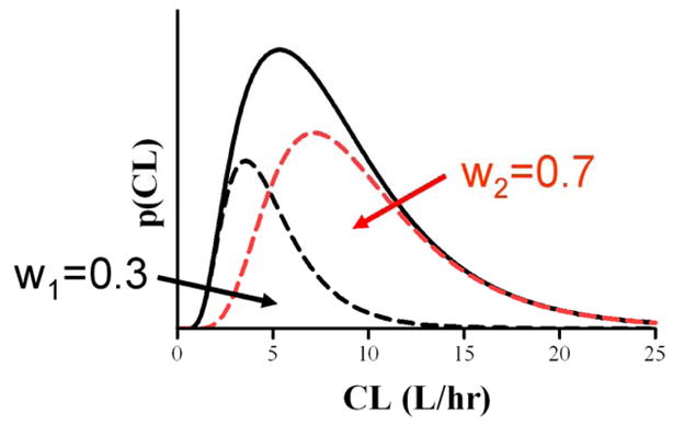
The model parameters V (L) and K_a (hr⁻¹) were assumed to be independent with $V_i{\sim }_{i.i.d.}LN({\mu }_V=50,{\sigma }_V^2={10}^2)$ and $K{a}_i{\sim }_{i.i.d.}LN({\mu }_{Ka}=1,{\sigma }_{Ka}^2={0.2}^2)$. The drug’s clearance CL (L/hr) was assumed to be a mixture of two lognormal densities:

$$C{L}_i{\sim }_{i.i.d.}{w}_{1}LN({\mu }_{C{L}_1}=5,{\sigma }_{C{L}_1}^2={(0.5{\mu }_{C{L}_1})}^2)+w_{2}LN({\mu }_{C{L}_2}=10,{\sigma }_{C{L}_2}^2={(0.5{\mu }_{C{L}_2})}^2)$$

with mixing weights w₁ =0.3 and w₂ =0.7. A sparse sampling schedule was used (m=4) with t₁ =2, t₂ =8, t₃ =12 and t₂₄ = 24 hrs. This is a difficult mixture problem, as is evident from inspection of the density for CL shown in Fig. 1, and was taken from a study of the kinetics of the drug metoprolol used by Kaila et al. (2006). The within individual error ε_ji is assumed to be i.i.d with σ² =0.1^2. The number of samples was reduced from the six sample times used by Kaila et al. (1, 2, 4, 8, 12, 24 hrs) to the four sample times used here in order to provide an even more challenging test. The number and timing of samples can influence estimation results and formal approaches to sample schedule design for population studies are available (Mentré et al., (1997)). A total of 300 population data sets were simulated from this model each consisting of n =50 subjects.

Fig. 1.

Simulated population density of clearance CL

The MAP estimates were obtained for each of the 300 population data sets using the EM algorithm with importance sampling as described above (the lognormal kinetic parameters were transformed). Very dispersed priors were assumed for the transformed parameters as follows:

$$\begin{array}{l}{\mu }_1\mid {\mathrm{\sum }}_1\sim N(log(5),{\mathrm{\sum }}_1/0.01){\mu }_2\mid {\mathrm{\sum }}_2\sim N(log(10),{\mathrm{\sum }}_2/0.01)\\ {({\mathrm{\sum }}_1)}^{-1}={({\mathrm{\sum }}_2)}^{-1}\sim \mathit{Wishart}(1,0.25)\\ (w_1,w_2)\sim \mathit{Dirichlet}(1,1)\\ {({\sigma }^2)}^{-1}\sim \mathit{Gamma}(1,0)\end{array}$$

For each of the estimated parametersφ, its percent prediction error was calculated for each population data set as:

$${\text{pe}}_j=100\times ({\phi }_j^{\text{MAP}}-{\phi }_j)/{\phi }_j,j=1,\dots ,300$$

These percent prediction errors were used to calculate the mean prediction error and root mean square prediction error (RMSE) for each parameter. In addition, the individual subject classification accuracy was evaluated for each population data set.

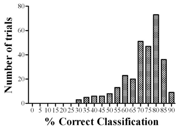
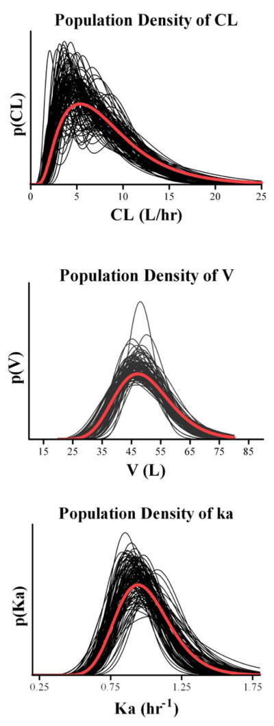
Figure 2 plots the estimated parameter population distributions of the 300 simulated data sets, as well as the true distributions used in the simulation, while Table 1 shows the mean estimates, estimation biases and root mean square errors (RMSE). The histogram of the percent correct classification is presented in Figure 3.

Fig. 2.

True (bold lines) and estimated (thin lines) population densities of CL (upper panel), V (middle panel) and Ka (lower panel).

Table 1.

True population values and mean of parameter estimates (300 trials), mean percent prediction error (PE) and root mean square percent prediction error (RMSE)

Parameter	Population Values	Mean of Estimates	Mean PE (%)	RMSE (%)
μCL1	5	5.177	3.541	30.50
μCL2	10	9.709	−2.910	20.55
μV	50	49.09	−1.816	3.374
μka	1	0.986	−1.401	6.287
σCL2 (cv%)	50	45.21	−18.25	36.79
σV2 (cv%)	20	19.31	−6.796	22.64
σka2 (cv%)	20	19.77	−2.270	42.25
w1	0.3	0.4486	49.53	68.44
σ	0.1	0.1094	9.421	15.46

Fig. 3.

Histogram of percent correct classification.

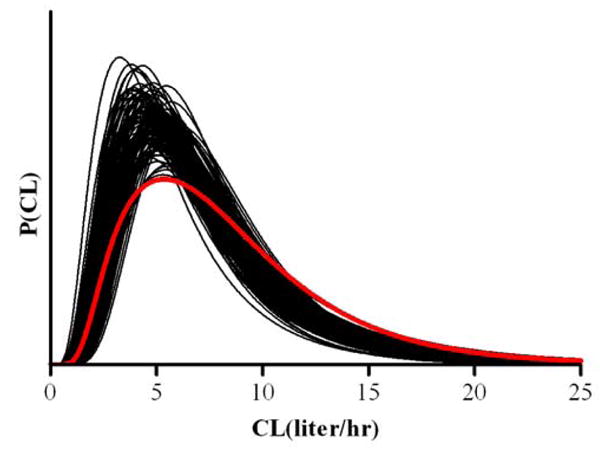
The data were also analyzed assuming a single component model for CL (lognormal) as well as for V and K_a as above. Model selection was based on the Bayesian information criterion (BIC) to select between a one or two component model for CL in each of the 300 population data sets. The estimated densities of clearance are displayed in Figure 4, while the detailed estimation results are given in Table 2. Based on BIC values, the two-component lognormal model for CL was correctly selected in 198 out of the 300 population trials.

Fig. 4.

True (bold lines) and estimated (thin lines) population densities of CL for the single component analysis

Table 2.

True population values and mean of parameter estimates (300 trials) for the single component model

Parameter	Population Values	Mean of Estimates
μCL1	5	7.271
μCL2	10	X
μV	50	49.16
μka	1	0.9891
σCL2 (cv%)	50	56.97
σV2 (cv%)	20	18.84
σka2 (cv%)	20	18.30
σ	0.1	0.1163

6. Discussion

In this paper, a maximum a posteriori probability estimation approach is presented for nonlinear random effects finite mixtures models that has application to identifying hidden subpopulations in pharmacokinetic/pharmacodynamic studies. Previously reported nonparametric Bayesian approaches to this problem (Wakefield and Walker (1997), Rosner and Mueller (1997)) have advantages over the MAP estimation approach presented herein, including calculation of the complete posterior distribution of model parameters including the number of mixing components. However, the computational challenges associated with the proper solution to the nonparametric Bayesian mixture problem are considerable, whereas the MAP estimation approach using the EM algorithm with importance sampling presented here is straightforward in comparison.

In calculating the MAP estimator, the values of the parameters defining the conjugate prior densities may be available from previous studies. When no prior information is available, these parameters can be set to reflect very disperse priors (e.g, τ_k → 0 and other parameters set as illustrated in the example presented). For linear mixture models with diffuse priors, as noted by Fraley and Raftery (2005), it is expected that the MAP results will be similar to the MLE results when they latter can be calculated. The advantage of the MAP estimator in such cases is that it avoids the unboundedness that can be associated with maximum likelihood mixture model problems (Fraley and Raftery (2005), Ormoneit and Tresp (1998)).

For determining the number of components in mixture models, several measures have been suggested, including the BIC criterion used in the example presented in this paper. In addition, a priori knowledge or assumptions about the biological mechanism for the modeled PK/PD polymorphism can also facilitate the model selection procedure, when combined with a model selection measure. For example, for drugs primarily metabolized by the liver, the information on hepatic cytochrome P450 family can help to decide a reasonable range for the number of clearance subgroups (e.g., K=3 accounting for extensive, intermediate, and poor metabolizer subpopulations) thus limiting the number of competing models to be tested.

Appendix: Asymptotic Properites

Let ${\phi }_n^{\mathit{MAP}}$ be the posterior mode of φ given Yⁿ. Assuming that there is a “true” parameter φ₀ which lies in the interior of the support of p(φ), it can be shown under suitable hypotheses that ${\phi }_n^{\mathit{MAP}}$ is consistent and asymptotically normal (White, 1994). However, from a Bayesian perspective, it is more natural to investigate the asymptotic behavior of the conditional density p(φ|Yⁿ). Under the assumptions stated below, it is found that p(φ|Yⁿ) is asymptotically normal with mean ${\phi }_n^{\mathit{MAP}}$. This gives another justification for calculating the MAP estimate.

This result is now stated more precisely. Assume that the Hessian matrix $A_n(\phi )=\frac{{\partial }^{2}logp(\phi \mid Y^n)}{\partial \phi \partial \phi }$ is invertible at $\phi ={\phi }_n^{\mathit{MAP}}$. Then given the regularity conditions of Philppou and Roussas (1975) and Bernardo and Smith (2001), it can be shown that ${\mathrm{\Gamma }}_n^{-1/2}({\phi }_n-{\phi }_n^{ML})$ converges in distribution to a standard multivariate normal random variable as n → ∞, where φ_n ~ p(φ|Yⁿ) and ${\mathrm{\Gamma }}_n^{-1}=-A_n({\phi }_n^{\mathit{MAP}})$. It follows that asymptotically, ${\phi }_n^{\mathit{MAP}}$ and Γ_n are the posterior mean and posterior covariance of p(φ|Yⁿ). For any component of ${\phi }_n^{\mathit{MAP}}$, the posterior standard error is the corresponding diagonal element of Γ_n.

The computation of Γ_n proceeds as follows:

$$\frac{{\partial }^{2}logp(\phi \mid Y^n)}{\partial \phi \partial \phi }=\left({\displaystyle \sum _{i=1}^n}\frac{{\partial }^{2}logp(Y_i\mid \phi )}{\partial \phi \partial \phi }\right)+\frac{{\partial }^{2}logp(\phi )}{\partial \phi \partial \phi }$$

and

$$-{\displaystyle \sum _{i=1}^n}\frac{\partial logp(Y_i\mid {\phi }_n^{\mathit{MAP}})}{\partial \phi \partial \phi }\approx {\displaystyle \sum _{i=1}^n}{V}_i({\phi }_n^{\mathit{MAP}})$$

where

$$V_i(\phi )=\frac{\partial logp(Y_i\mid \phi )}{\partial \phi }{(\frac{\partial logp(Y_i\mid \phi )}{\partial \phi })}^T$$

It follows that

$${\mathrm{\Gamma }}_n\approx {\left({\displaystyle \sum _{i=1}^n}{V}_i({\phi }_n^{\mathit{MAP}})-\frac{{\partial }^{2}logp({\phi }_n^{\mathit{MAP}})}{\partial \phi \partial \phi }\right)}^{-1}.$$

Note that in the maximum likelihood setting of Wang et al (2007), $\mathit{Cov}({\phi }_n^{ML})\approx {\left({\displaystyle \sum _{i=1}^n}{V}_i({\phi }_n^{\mathit{MAP}})\right)}^{-1}$. So the difference between MAP and ML is the term $\frac{{\partial }^{2}logp({\phi }_n^{\mathit{MAP}})}{\partial \phi \partial \phi }$. As n → ∞, the contribution of this term diminishes.

In this asymptotic analysis the precisions (σ²)⁻¹ and ${\mathrm{\sum }}_k^{-1}$ are considered as primary variables instead of the variances σ² and Σ_k. This is standard practice in the normal, gamma, Wishart model. Further using ${\mathrm{\sum }}_k^{-1}$ instead of Σ_k greatly simplifies the second derivative calculations.

We first calculate V_i(φ), i =1, …, n. The formulas below are similar to those given in given in Wang, et al (2007). The gradient components are calculated using the relation:

$$\frac{\partial }{\partial \phi }logp(Y_i\mid \phi )={\displaystyle \sum _{k=1}^K}\int \{\frac{\partial }{\partial \phi }logp(Y_i\mid \phi ,\gamma )w_k\eta (\theta \mid {\mu }_k,{\mathrm{\sum }}_k)\}{g}_{ik}({\theta }_i,\phi )d\theta ,$$

We have:

$$s_{{({\sigma }^2)}^{-1}}=\frac{\partial }{\partial {({\sigma }^2)}^{-1}}logp(Y_i\mid \phi )={\displaystyle \sum _{k=1}^K}\int \{(1/2)m_i{\sigma }^2-(1/2){(Y_i-h_i(\theta ))}^T{H}_i{(\theta )}^{-1}(Y_i-h_i(\theta )\}{g}_{ik}(\theta ,\phi )d\theta$$

Next using the constraint: w_K = 1 – w₁ – … – w_K−1, we have for k =1, …, K − 1

$$s_{w_k}=\frac{\partial }{\partial w_k}logp(Y_i\mid \phi )=\frac{1}{w_k}\int g_{ik}(\theta ,\phi )d{\theta }_i-\frac{1}{w_K}\int g_{iK}(\theta ,\phi )d\theta .$$

And for k =1, …, K

$$\begin{array}{l}{s}_{{\mu }_k}=\frac{\partial }{\partial {\mu }_k}logp(Y_i\mid \phi )=\int g_{ik}(\theta ,\phi )\{{{\mathrm{\sum }}_k}^{-1}(\theta -{\mu }_k)\}d\theta ,\\ \frac{\partial }{\partial {\mathrm{\sum }}_k^{-1}}logp(Y_i\mid \phi )=\int \{(1/2){\mathrm{\sum }}_k-(1/2)(\theta -{\mu }_k){(\theta -{\mu }_k)}^T\}{g}_{ik}(\theta ,\phi )d\theta ,\end{array}$$

so that

$$s_{\mathit{vech}({\mathrm{\sum }}_k^{-1})}=\frac{\partial }{\partial \mathit{vech}({\mathrm{\sum }}_k^{-1})}logp(Y_i\mid \phi )=\mathit{vech}[2\frac{\partial }{\partial {\mathrm{\sum }}_k^{-1}}logp(Y_i\mid \phi )-\mathit{Diagonal}(\frac{\partial }{\partial {\mathrm{\sum }}_k^{-1}}logp(Y_i\mid \phi ))]$$

where vech(X) is the vector of the lower triangular components of a symmetric matrix X. Putting these results together produces the vector

$$s_i=(s_{{({\sigma }^2)}^{-1}},s_{w_1},\dots ,s_{w_{K-1}},s_{{\mu }_1},\dots ,s_{{\mu }_K},s_{\mathit{vech}({\mathrm{\sum }}_1^{-1})},\dots ,s_{\mathit{vech}({\mathrm{\sum }}_K^{-1})}),$$

and the formula

$$V_i(\phi )={({\displaystyle \sum _{i=1}^n}{s}_i{s_i}^T)}^{-1}.$$

All the above computations can be performed during the importance sampler calculation at the final iteration of the EM algorithm.

It remains to calculate $\frac{{\partial }^{2}logp(\phi )}{\partial \phi \partial \phi }$. For this calculation we represent the parameter φ as $\phi =\{{({\sigma }^2)}^{-1},w_1,\dots ,w_{K-1},({\mu }_k,{\mathrm{\sum }}_k^{-1}),k=1,\dots ,K\}$. Now supposeθ has p components. Then each μ_k has p components and each ${\mathrm{\sum }}_k^{-1}$ has p(p+1)/2 unique components. Therefore $\frac{{\partial }^{2}logp(\phi )}{\partial \phi \partial \phi }$ is an R×R matrix, where R = 1 + (p − 1) + Kp + Kp(p+1)/2. Now

$$logp(\phi )=logp({\sigma }^{-2})+logp(w_1,\dots w_{K-1})+{\sum }_{k=1}^{K}logp({\mu }_k\mid {\mathrm{\sum }}_k^{-1})+{\sum }_{k=1}^{K}logp({\mathrm{\sum }}_k^{-1})$$

so that $B=\frac{{\partial }^{2}logp(\phi )}{\partial \phi \partial \phi }$ is a block diagonal matrix of the form B =Diag (B_σ⁻²; B_w; B(_μkνk), k =1, …, K), ${\nu }_k=\mathit{vech}({\mathrm{\sum }}_k^{-1})$.

To calculate B the following parameterizations for the prior p(φ) are assumed:

$$\begin{array}{l}p(\kappa )=c{\kappa }^{(a-1)}exp(-b\kappa ),\kappa ={\sigma }^{-2}\\ p(w_1,\dots ,w_{K-1})=c{(w_1)}^{a_1-1}\cdots ·{(w_K)}^{a_K-1},w_K=1-(w_1+\dots +w_{K-1})\\ p({\mu }_k\mid {\mathrm{\sum }}_k^{-1})=C{(det{\mathrm{\sum }}_k^{-1})}^{1/2}exp((-{\tau }_k/2){({\mu }_k-{\lambda }_k)}^T{\mathrm{\sum }}_k^{-1}({\mu }_k-{\lambda }_k)\\ p({\mathrm{\sum }}_k^{-1})=C{(det{\mathrm{\sum }}_k^{-1})}^{\beta }exp(-tr({\mathrm{\Psi }}_k{\mathrm{\sum }}_k^{-1})/2),\beta =(q_k-d-1)/2\end{array}$$

It follows:

$$\begin{array}{l}{B}_{{\sigma }^{-2}}=\frac{{\partial }^2}{\partial {\sigma }^{-2}\partial {\sigma }^{-2}}logp({\sigma }^{-2})=-(a-1){\sigma }^4\\ B_w=\frac{{\partial }^2}{\partial w\partial w}logp(w),w=(w_1,\dots ,w_{K-1})\\ {[B_w]}_{rr}=-(a_r-1)/{(w_r)}^2+(a_K-1)/{(w_K)}^2,r=1,\dots ,p-1\\ {[B_w]}_{rs}=(a_K-1)/{(w_K)}^2,1\le r,s\le p-1,r\ne s\\ B_{({\mu }_k,v_k)}=\left[\begin{array}{cc}{G}_{p\times p}& H_{p\times p(p+1)/2}\\ H^T& J_{p(p+1)/2\times p(p+1)/2}\end{array}\right]\\ G=\frac{{\partial }^2}{\partial {\mu }_k\partial {\mu }_k}logp({\mu }_k\mid {\mathrm{\sum }}_k^{-1})=-{\tau }_k{\mathrm{\sum }}_k^{-1}\\ H=\frac{{\partial }^2}{\partial {\mu }_k\partial \mathit{vech}({\mathrm{\sum }}_k^{-1})}logp({\mu }_k\mid {\mathrm{\sum }}_k)=-{\tau }_k{D}^T(({\mu }_k-{\lambda }_k)\otimes I)D,\\ J=J_1+J_2\\ J_1=\frac{{\partial }^2}{\partial \mathit{vech}({\mathrm{\sum }}_k^{-1})\partial \mathit{vech}({\mathrm{\sum }}_k^{-1})}logp({\mu }_k\mid {\mathrm{\sum }}_k^{-1})=-(1/2)D^T{\mathrm{\sum }}_k\otimes {\mathrm{\sum }}_{k}D\\ J_2=\frac{{\partial }^2}{\partial \mathit{vech}({\mathrm{\sum }}_k^{-1})\partial \mathit{vech}({\mathrm{\sum }}_k^{-1})}logp({\mathrm{\sum }}_k)=-\beta D^T{\mathrm{\sum }}_k\otimes {\mathrm{\sum }}_{k}D\end{array}$$

In the above equations, D is the permutation matrix satisfying D vech (X) =vec (X), where vec (X) is the vector of the stacked columns of the symmetric matrix X, and ⊗ is the Kronecker product (see Minka (2000)).

References

- Bernardo JM, Smith AFM. Bayesian Theory, Section 5.3.2. Wiley; New York: 2001. [Google Scholar]
- Cruz-Mesía R, Quintana FA, Marshall G. Model-based clustering for longitudinal data. Computational Statistics & Data Analysis. 2008;52:1441–1457. [Google Scholar]
- Dempster AP, Laird N, Rubin DB. Maximum likelihood from incomplete data via the EM algorithm. J Roy Statist Soc B. 1977;39:1–38. [Google Scholar]
- Evans WE, Relling MV. Pharmacogenomics: Translating functional genomics into rational therapeutics. Science. 1999;286:487–491. doi: 10.1126/science.286.5439.487. [DOI] [PubMed] [Google Scholar]
- Fraley C, Raftery AE. Technical Report no. 486. Department of Statistics, University of Washington; 2005. Bayesian regularization for Normal mixture estimation and model-based clustering. http://handle.dtic.mil/100.2/ADA454825. [Google Scholar]
- Gelfand AE, Smith AFM. Sampling-based approaches to calculating marginal densities. J of the Am Stat Assoc. 1990;85:398–409. [Google Scholar]
- Katz D, Azen SP, Schumitzky A. Bayesian approach to the analysis of nonlinear models: Implementation and evaluation. Biometrics. 1981;37:137–142. [Google Scholar]
- Kaila N, Straka RJ, Brundage RC. Mixture models and subpopulation classification: a pharmacokinetic simulation study and application to metoprolol CYP2D6 phenotype. J Pharmacokinet Pharmacodyn. 2007;34:141–156. doi: 10.1007/s10928-006-9038-9. [DOI] [PubMed] [Google Scholar]
- Lemenuel-diot A, Laveille C, Frey N, Jochemsen R, Mallet A. Mixture modeling for the detection of subpopulations in a pharmacokinetic/pharmacodynamic analysis. J Pharmacokinet Pharmacodyn. 2006;34:157–181. doi: 10.1007/s10928-006-9039-8. [DOI] [PubMed] [Google Scholar]
- Lunn DJ, Best N, Thomas A, Wakefield J, Spiegelhalter D. Bayesian analysis of population PK/PD models: general concepts and software. J of Pharmacokin and Pharmacodyn. 2002;29:217–307. doi: 10.1023/a:1020206907668. [DOI] [PubMed] [Google Scholar]
- Mentré F, Mallet A, Baccar D. Optimal design in random effect regression models. Biometrika. 1997;84:429–442. [Google Scholar]
- Minka T. Old and new matrix algebra useful for statistics. MIT Media Lab. 2000 http://research.microsoft.com/minka/papers/matrix.
- Ormoneit D, Tresp V. Averaging, maximum penalized likelihood and Bayesian estimation for improving Gaussian mixture probability density estimates. IEEE Transactions on Neural Networks. 1998;9:639–650. doi: 10.1109/72.701177. [DOI] [PubMed] [Google Scholar]
- Pauler DK, Laird NM. A mixture model for longitudinal data with application to assessment of noncompliance. Biometrics. 2000;56:464–472. doi: 10.1111/j.0006-341x.2000.00464.x. [DOI] [PubMed] [Google Scholar]
- Racine-Poon A. A Bayesian approach to non-linear random effects models. Biometrics. 1985;41:1015–1024. [PubMed] [Google Scholar]
- Rosner GL, Muller P. Bayesian population pharmacokinetic and pharmacodynamic analyses using mixture models. J Pharmacokinet Biopharm. 1997;2:209–234. doi: 10.1023/a:1025784113869. [DOI] [PubMed] [Google Scholar]
- Sheiner LB, Halkin H, Peck C, Rosenberg B, Melmon KL. Improved computer assisted digoxin therapy: a method using feedback of measured serum digoxin concentrations. Ann Intern Med. 1975;82:619–627. doi: 10.7326/0003-4819-82-5-619. [DOI] [PubMed] [Google Scholar]
- Tseng P. An analysis of the EM algorithm and entropy-like proximal point methods. Math Oper Res. 2005;29:27–44. [Google Scholar]
- Wakefield JC, Smith AFM, Racine-Poon A, Gelfand AE. Bayesian analysis of linear and non-linear population models by using the Gibbs sampler. Applied Statistics. 1994;43:201–221. [Google Scholar]
- Wakefield JC, Walker SG. Bayesian nonparametric population models: formulation and comparison with likelihood approaches. J Pharmacokinet Biopharm. 1997;25:235–253. doi: 10.1023/a:1025736230707. [DOI] [PubMed] [Google Scholar]
- Wang X, Schumitzky A, D’Argenio DZ. Nonlinear random effects mixture models: Maximum likelihood estimation via the EM algorithm. Comput Stat Data Anal. 2007;51:6614–6623. doi: 10.1016/j.csda.2007.03.008. [DOI] [PMC free article] [PubMed] [Google Scholar]
- White H. Estimation, Inference and Specification Analysis. Cambridge University Press; 1994. Chapter 6. [Google Scholar]
- Wu CF. On the convergence properties of the EM algorithm. Ann Stat. 1983;11:95–103. [Google Scholar]