

Abstract
The inverse relationship between the incidence and the average age of first infection for immunizing agents has become a basic tenet in the theory underlying the mathematical modeling of infectious diseases. However, this relationship assumes that the infection has reached an endemic equilibrium. In reality, most infectious diseases exhibit seasonal and/or long-term oscillations in incidence. We use a seasonally-forced age-structured SIR model to explore the relationship between the number of cases and the average age of first infection over a single epidemic cycle. Contrary to the relationship for the equilibrium dynamics, we find that the average age of first infection is greatest at or near the peak of the epidemic when mixing is homogeneous. We explore the sensitivity of our findings to assumptions about the natural history of infection, population mixing behavior, the mechanism of seasonality, and of the timing of case reporting in relation to the infectious period. We conclude that seasonal variation in the average age of first infection tends to be greatest for acute infections, and the relationship between the number of cases and the average age of first infection can vary depending on the nature of population mixing and the natural history of infection.
Keywords: epidemic model, age distribution, seasonality
1. Introduction
Age-structured epidemic models have long been used to understand how transmission of infections might vary among different age groups. These models were originally developed to provide insight into how policies such as vaccination affect the age distribution of infection (Griffiths, 1974; Schenzle, 1984). The long-term dynamics of such models are relatively well understood. It has been shown that at equilibrium, the average age of first infection is inversely proportional to the force of infection (λ), and thus the incidence of disease (Anderson and May, 1983; Anderson and May, 1985; Dietz, 1975). This is consistent with observations that the mean age of infection with a number of childhood diseases was lower in urban compared to rural areas (Fales, 1928), and that the average age of pediatric patients with mild and severe clinical malaria decreased with increasing transmission intensity in sub-Saharan Africa (Snow and Marsh, 1998). Interventions that reduce the incidence of infection, such as vaccination, are expected to lead to an increase in the average age of infection (Griffiths, 1973). This is a trend that has been observed for poliomyelitis in association with improved hygiene in the U.S. (Anderson and May, 1991) and for post-vaccination measles, rubella, and pertussis (Anderson and May, 1991; Broutin et al., 2005).
However many infections do not reach an endemic equilibrium, but rather exhibit regular epidemic cycles due to the interaction between susceptible and infectious hosts. In the absence of stochastic effects or seasonal forcing, the basic SIR (susceptible-infectious-recovered) family of models predict that these oscillations will be damped until a stable endemic equilibrium is reached (Anderson and May, 1991). Seasonal variations in climatic factors, immune system function, and/or population contact rates help sustain these oscillations (Dowell, 2001; Grassly and Fraser, 2006). These seasonal variations in epidemic parameters generally occur with a period of 1 year, but the period of the long-term oscillations in disease incidence due to the dynamical interaction of susceptible and infected hosts may be annual or multi-annual. If the natural period of oscillations is an approximate linear multiple of the 1-year seasonal forcing, then resonance can lead to large-amplitude fluctuations in the number of infections at the underlying sub-harmonic frequency (Dietz, 1976). Certain aspects of short-term dynamics have also been studied extensively, such as the effect of age-structure on the periodicity of oscillations in incidence and the tendency of such models to exhibit chaos (Bolker and Grenfell, 1993; Earn et al., 2000; Earn et al., 1998; Olsen and Schaffer, 1990; Rohani et al., 1999). Relatively little attention, however, has been paid to short-term seasonal changes in the average age of infection predicted by such models.
Hitherto, most researchers have ignored seasonal changes in the age distribution of infection, or have assumed that such changes reflected seasonal differences in mixing patterns, primarily due to school terms (Bolker and Grenfell, 1993; Grenfell and Anderson, 1985). While the presence of seasonal or regular epidemics has been shown to have little impact on the estimation of certain parameters important in determining the long-term dynamics (Whitaker and Farrington, 2004), examining the relationship between the number of cases and the average age of first infection may help to provide additional insight into the etiology of diseases for which the involvement of an infection has been hypothesized, but for which a specific infectious agent has yet to be identified. One such disease is Kawasaki disease (KD), an acute systemic vasculitis that occurs primarily in children under 5 years of age. Two aspects of the epidemiologic evidence which suggest an infectious etiology for KD include seasonal fluctuations in incidence and the age distribution of cases (Burgner and Harnden, 2005). If one assumes that an infectious agent is responsible for KD, then by examining the correlation between the number of cases and the average age of such cases, it may be possible to predict the values of certain parameters of that infectious agent, such as the duration of infectiousness and the nature of immunity to re-infection. Comparing these predictions against measured values for candidate etiologic agents could help to narrow the range of possibilities, providing a source of evidence independent of the types of evidence usually considered in identifying etiology.
We define a basic age-structured SIR model and examine how the relationship between the number of cases and the average age of first infection varies for an immunizing infection depending on the duration of infectiousness and assumptions about population mixing. We find that the average age of first infection is greatest at or soon after the epidemic peak regardless of the duration of infectiousness when we assume homogeneous mixing. This relationship emerges as a consequence of fluctuations in the susceptible population, and can be verified mathematically under some simplifying assumptions. We go on to explore how sensitive this relationship is to assumptions about population mixing, the mechanism of seasonality, the presence of a latent period prior to onset of infectiousness, and whether we consider prevalent or incident infections to be more representative of case report data.
2. Basic age-structured SIR model
2.1. Description of the model
We first define a basic age-structured SIR model. We model a hypothetical population in which individuals are equally divided among 80 one-year age classes. Individuals are born into the first susceptible age class (S1) at a rate of ν = 12.6 births per 1,000 people per year, and age into the next age class at a rate μ = 1 yr-1. All individuals live to 80 years old, at which point they die (or are dropped from the model), leading to a rectangular age distribution that approximates that of a developed country (Anderson and May, 1983). Movement of individuals from one age class to the next and from one infection state to another is governed by a series of differential equations.
The SIR model assumes that individuals become immediately infectious upon disease transmission, and that infection is immunizing, such that once an infected individual has recovered, he/she is immune to re-infection later in life. The set of ordinary differential equations (ODEs) that describe the system are as follows:
| (2.1) |
where Si, Ii, and Ri are the number susceptible, infectious, and recovered (respectively) in age class i, μ is the rate of aging out of age class i, and δ is the rate of recovery from infection (=1/D, where D is the duration of infectiousness). Note that all individuals are born into the susceptible class, such that μS0 = ν (the birth rate) and μI0 = μR0 = 0.
The force of infection for age class i at time t (measured in weeks) is given by
| (2.2) |
where b1 is the relative amplitude of seasonal forcing and βij is transmission parameter for transmission from age group j to age group i, which is the product of the age-specific contact rate (the proportion of the population in age group j contacted by an individual in age group i in a given week) and the probability of transmission given contact. Initially, we assume mixing is homogeneous, such that all individuals are equally likely to contact one another regardless of age; thus βij = β and λi(t) = λ(t) do not depend upon the age of individuals. We explore the sensitivity of our results to this assumption in Section 3.
For convenience, we model age using discrete age classes rather than treating age as a continuous variable. The small (1-year) width of the age classes should limit problems associated with assuming exponential rates of aging (such that some individuals spend much less than a year in a given age class, while others spend >1 year), since the variance in the time spent in a given age class relative to the mean will decrease when aggregated over multiple years (e.g. when aggregated over 5 years, the distribution of time spent within any 5-year age group is Γ(5,1), and approximately 90% of density lies between 2 and 9 years). However, to ensure our results are not sensitive to this assumption, we further subdivide the population into monthly age groupings for 0-10 years of age, such that the time spent in any 12-month age grouping is Γ(12,1) (90% CI 6.9-18.2 months).
We vary the duration of infectiousness (D) from 1 week to 12 weeks. The probability of infection per contact in the model is adjusted such that βD remains the same and the average age of infection is between 4-6 years old, consistent with the mean age of Kawasaki disease cases in the U.S., as well as a number of childhood infections including measles and pertussis in the pre-vaccination era (Anderson and May, 1991). The ODEs were integrated using the Dormand-Prince method in MATLAB v7.6 (The MathWorks, Natick, MA). The full code is available from the authors upon request.
2.2. Analysis of the relationship between the number cases and average age of first infection
We assess the relationship between the number of incident infections and the average age of such infections over a period of 10 years once the model has reached an “equilibrium” annual or multi-annual cycle. Let and be the total number of susceptible and infectious individuals, respectively, at time t, and recall that when we assume homogeneous mixing. The number of incident infections at time t is and the average age of cases is given by
| (2.3) |
where the weight ai is the midpoint of age group i. Thus, under homogeneous mixing, the average age of incident cases is equal to the average age of susceptible individuals in the population.
We calculate Pearson correlation coefficients between the total number of cases at time t, C(t), and the average age of first infection at time t+l, A(t+l), where the lag time l varies from 0 to T − 1 weeks, where T is the period of oscillations predicted by the model. The outcome variables are the lag time associated with the maximum correlation (which can also be interpreted approximately as the number of weeks between the peak in the number of cases and the peak in the average age of infection), the correlation coefficient for lag l = 0 (ρ0), and the difference between the maximum and minimum average age of infection (Amax − Amin).
2.3. Homogeneous mixing results and discussion
We find that when the duration of infectiousness is short (D = 1 week), the average age of first infection reaches its maximum at the same time as the peak in the number of cases (l = 0 weeks) and the average age of infection and the number of cases are positively correlated (ρ0 = 0.850) (Table 1). As the duration of infectiousness increases, the lag time and the correlation remain approximately the same; again the average age of first infection reaches a maximum at or within 1 week of the peak in the number of cases (Table 1). The difference between the maximum and minimum average age of first infection (Amax − Amin) is greatest when D = 1 week, but diminishes substantially (to levels that may be unmeasurable in practice) as the duration of infectiousness increases. However, note that the magnitude of seasonal forcing (which is largely unknown) affects the amplitude of seasonal variation in the average age of first infection, but does not have much of an effect on the lag time or ρ0 (Table 1).
Table 1.
Age-structured model results for the relationship between the number of incident cases (C) and the average age of first infection (A) for the basic SIR model assuming homogeneous mixing.
| Outcome measure | Duration of infectiousness | |||
|---|---|---|---|---|
| 1 week | 4 weeks | 8 weeks | 12 weeks | |
| Lag time | 0c | 0 | 0 | 0 |
| ρ0 | 0.840 | 0.983 | 0.992 | 0.988 |
| Amax - Amina | 0.087 | 0.002 | 0.001 | 0.001 |
| Amax - Aminb | --d | 0.008 | 0.005 | 0.004 |
Seasonal forcing = 5%
Seasonal forcing = 25%
Epidemic period = 2 years
Epidemic fade-out occurred
Examining how the proportion susceptible within each age group and the age distribution of cases changes over the course of a single epidemic helps us to understand why this occurs. For acute infections (D = 1 week), the proportion of susceptible individuals in each age group is increasing during the period of low incidence (Fig. 1a); more susceptible individuals are being born into the youngest age class or aging into the older age classes than are being infected within each age group. The proportion susceptible within the youngest age class begins to decline slightly sooner than that of the older age classes (and prior to the peak of the epidemic) because the build-up of susceptibles has been greatest within the youngest age class. Following the peak of the epidemic, the proportion susceptible within the youngest age class begins to increase again quite a bit sooner than that of the other age classes, since individuals are born into S1 at a constant rate, but age into the older susceptible age classes at a slightly slower rate since there are fewer susceptibles remaining in the next youngest age class following the epidemic. As a result, the proportion of cases occurring among members of the youngest age class begins to increase (and the average age of first infection begins to decrease) following the peak of the epidemic (Fig. 1b). Thus, when the duration of infectiousness is short, the proportion of cases occurring within the youngest age group is higher during the trough and lowest at the peak of the epidemic. This leads to a positive correlation between the number of cases and the average age of first infection.
Figure 1.
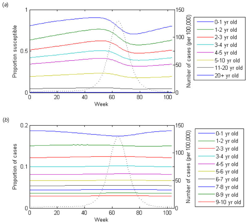
Dynamics of the basic SIR model over a single epidemic cycle for an acute infection (D = 1 week, 5% seasonal forcing). (a) The proportion of the age group susceptible to infection. (b) The proportion of cases occurring among each age group is indicated by the colored lines. The dotted lines represent the incidence of infection.
For longer durations of infectiousness (D = 12 weeks), however, there is less seasonal fluctuation in the proportion susceptible within each age group (Fig. 2a). The number of cases tends to be more constant throughout the year, even with stronger seasonal forcing. The rate of epidemic spread is slower; in order for the average age of first infection to remain around 4-6 years old, the per day probability of transmission given contact between a susceptible and infectious individuals must be less. However, members of the youngest age groups still tend to be infected early on in the epidemic, leaving fewer susceptibles (and therefore a smaller proportion of cases) in the youngest age class by the peak of the epidemic. Under some simplifying assumptions, it is possible to show that these findings are general and to understand mathematically how they are generated (Appendix A).
Figure 2.
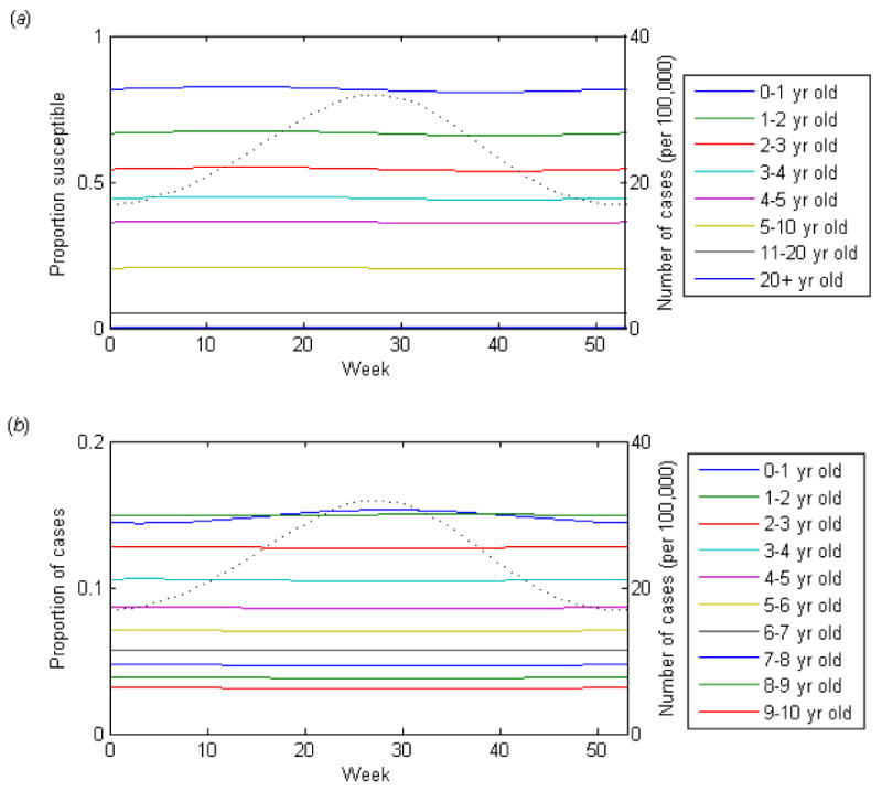
Dynamics of the basic SIR model over a single epidemic cycle for a long duration infection (D = 12 weeks, 25% seasonal forcing). (a) The proportion of the age group susceptible to infection. (b) The proportion of cases occurring among each age group is indicated by the colored lines. The dotted line represents the incidence of infection.
3. Sensitivity to population mixing assumptions
We explore a variety of assumptions about how individuals belonging to different age classes mix with one another, and construct “who acquires infection from whom” (WAIFW) matrices based on these assumptions (Appendix B). The simplest assumption is that individuals are equally likely to contact any other individual in the population regardless of age (homogeneous mixing), which we explored in Section 2. Alternatively, we might assume that individuals are 10-times more likely to contact other members of their own age class (assortative mixing), such that βii = 10βij for i≠j. We expect this to be a slightly better (albeit over-simplified) reflection of the true population mixing behavior for respiratory-transmitted infections, as individuals tend to have more contact with others their own age, particularly within the setting of schools.
However, the reality is likely somewhere in between. Recent studies have attempted to estimate age-specific transmission parameters for respiratory infections using a combination of serologic data and self-reported contact data (Mossong et al., 2008; Wallinga et al., 2006). Participants in the study were asked to report the number and approximate age (within 6- to 20-year age categories) of different individuals with whom they conversed in a typical week. The data was then corrected for reciprocity. Seroprevalence data was then used to estimate a disease-specific infectivity parameter (which was assumed to be independent of age), and to test the model fit. We use normalized age-specific contact rates from the Netherlands (Wallinga et al., 2006) (self-reported mixing). These are in broad agreement with estimates from other European countries (Mossong et al., 2008).
Finally, others have attempted to estimate age-specific transmission parameters from serological data and case reports by constraining certain parameters to be equal to one another. One such matrix used to describe measles dynamics in England and Wales in the pre-vaccination era assumes that primary school children (6-10 years old) have a unique (and considerably higher) rate of mixing with one another than with other age groups (Anderson and May, 1985). Pre-school aged children have a relatively unique (and slightly elevated) rate of mixing with one another and with primary school children, while adolescents and adults each mix with other age groups at a uniform rate. Models utilizing such a matrix have been termed “realistic age-structured” (RAS) models; we use a matrix that is proportional to the estimates for one such model (Bolker and Grenfell, 1993) (RAS mixing). For all alternative mixing assumptions, we again adjust the probability of transmission per contact such that the average age of infection is approximately 4-6 years old.
The lag times are greater (12-24 weeks) and ρ0 is less for assortative and self-report mixing models (Table 2). For assortative mixing, there is a relatively strong dependence between the lag time and the duration of infectiousness; as the duration of infectiousness increases, so does the lag time between the peak in the number of cases and the average age of first infection. For long durations of infectiousness (D = 12 weeks), the number of cases and the average age of first infection are inversely correlated, such that cases tend to be younger at the peak of the epidemic and older during the trough. The lag time also increases slightly with longer durations of infectiousness for self-reported mixing, but the relationship is not as strong. When we assume primary school children mix with each other at much higher rates, as in the RAS model, the average age of infection is greatest prior to the peak in the number of cases (l = 40-41 weeks) and ρ0 is close to zero (Table 2). Furthermore, this type of population mixing leads to a slightly different age distribution of cases compared to the other mixing assumptions, with a large proportion of cases among those aged 6-10 years. The degree of seasonal variation in the average age of first infection is considerably higher under all alternative mixing assumptions compared to homogeneous mixing, and again tends to be greatest for acute infections.
Table 2.
Sensitivity of age-structured model results to population mixing assumptions for the SIR model.
| Mixing assumption (WAIFW) |
Outcome measure | Duration of infectiousness | |||
|---|---|---|---|---|---|
| 1 week | 4 weeks | 8 weeks | 12 weeks | ||
| Assortative | Lag time | 12 | 16 | 20 | 24 |
| ρ0 | 0.110 | -0.323 | -0.766 | -0.975 | |
| Amax - Amina | 0.303 | 0.209 | 0.084 | 0.051 | |
| Self-report | Lag time | 14b | 14 | 16 | 17 |
| ρ0 | 0.113 | -0.184 | -0.358 | -0.424 | |
| Amax - Amin | 0.938 | 0.142 | 0.075 | 0.055 | |
| RAS | Lag time | 40 | 41 | 41 | 40 |
| ρ0 | 0.086 | 0.234 | 0.201 | 0.133 | |
| Amax - Amin | 0.165 | 0.131 | 0.068 | 0.057 | |
Seasonal forcing = 5% for D = 1 week, 25% for D = 4-12 weeks
Epidemic period = 2 years
Intuitively it seems understandable that the average age of infection might be expected to vary over the course of the epidemic when population mixing is not homogeneous. If population mixing is highly assortative and members of the youngest age class are again the first to be infected at the beginning of an epidemic (since they have the greatest proportion susceptible and the highest rate of replenishment of susceptibles), then they will be more likely to infect other members of their own age class rather than a member of another age class. The proportion of cases occurring among the youngest age class will increase early in the epidemic. Some members of other age classes will be infected as well, with individuals from the younger age classes more likely to be infected than members of the older age classes due to variations in the proportion susceptible. This will lead to a gradual “spillover” of infection from one age class to the next, with the older age classes representing a greater proportion of the cases on the tail-end of the epidemic. Thus, for acute infections, the average age of infection peaks approximately 12 weeks after the peak in the number of cases. However, for longer durations of infectiousness, this spillover from one age class to the next occurs more gradually, leading to a greater lag time between the peak in the number of cases and the average age of first infection.
Realistic mixing based on self-reported contact data presents a similar scenario. Again, individuals are more likely to contact other members of their own age group, although in this case the age groupings are slightly larger (i.e. 6-year to 20-year age classes) and we assume homogeneous mixing within one's own age group. However, school-aged children and young adults have approximately 50% more contacts compared to pre-school children (age 0-5 years), and older adults. Thus, slightly more cases occur among school-aged children than predicted under homogeneous or assortative mixing. Again, the youngest children represent the largest proportion of cases at the beginning of the epidemic, while the proportion of cases occurring among older children increases following the peak of the epidemic.
Like the self-reported mixing behavior, the RAS models assume that school-aged children have more contacts than preschool children. In this case, however, the discrepancy is much larger; the contact rate among primary school children (age 6-10 years) is assumed to be almost 8 times higher than among pre-school children (age 0-5 years) and more than 30 times higher than among adults. As a result, the epidemic tends to begin among the primary school children despite the higher rates of immunity in these older age groups. Thus, the proportion of cases occurring among children 6 years of age and older increases towards the beginning of the epidemic then declines prior to the peak of the epidemic.
4. Mechanism of seasonality
The means by which seasonal oscillations in the incidence of infectious diseases are generated is largely unknown, although there are numerous hypotheses. Climatic factors such as colder temperatures and lower relative humidity (Lowen et al., 2007), host physiological factors such as photoperiod effects on levels of vitamin D (Cannell et al., 2006), and behavioral factors such as the aggregation of children in schools (Fine and Clarkson, 1982) have all been cited as possible causes of the seasonality of respiratory pathogens (Altizer et al., 2006; Dowell, 2001; Grassly and Fraser, 2006).
Sinusoidal forcing functions such as the one in Eq. (2.2) are often used to parameterize the underlying mechanism of seasonality. This parameterization seems appropriate if one assumes that climatic and/or host physiological factors are the primary drivers of the seasonal oscillations. However, other models, particularly the RAS models for measles dynamics, have considered the aggregation of children in schools to be the primary mechanism by which seasonal oscillations are generated (and longer-period oscillations are sustained) (Schenzle, 1984). Such models explicitly parameterize this using “term-time forcing” in which the contact rate among school-aged children (6-10 year olds) switches between a high in-school rate and a lower rate during school holidays. This type of seasonal forcing will likely impact the relationship between seasonal changes in incidence and the average age of infection since increased rates of transmission are associated with age-dependent changes in contact rates.
We examine how the use of term-time forcing affects the relationship between the number of cases and the average age of first infection. We use a formulation similar to that of Schenzle (1984) in which the contact rate among 6-10 year olds is equal to βij(1 + b2H(τ)), where τ = t mod 52 (measured in weeks), and the indicator function H(τ) for 0 ≤ τ < 52 is equal to 1 when school is in session and 0 during the winter, spring, summer, and fall vacation periods as follows:
| (4.1) |
We vary b2 such that the mixing rate among school-aged children was 2 to 8 times the rate of mixing among pre-school (0-5 year old) children, depending on the mixing assumption.
We examine the affect of term-time forcing for both the self-reported and RAS mixing assumptions. For self-reported mixing, we assume that the contact rate among school-aged (6-19 year old) children is the same as that among school-aged children during vacation periods, and that the in-school rate is 2 times higher for 6-12 year old children and 1.5 times higher for 13-19 year olds, leading to average annual rates similar to those of Wallinga, et al (2006). For RAS mixing, we use an in-school mixing rate similar to that of Bolker and Grenfell (1993) in which the mixing rate among school-aged children is approximately 8 times higher than during vacation periods, when it is assumed to be the same as that among pre-school aged children.
When we use term-time forcing to induce seasonal oscillations, we find that the average age of first infection is largely determined by the forcing function H(t), i.e. whether or not school was in session, regardless of the duration of infectiousness and population mixing assumption. The average age of infection tends to be higher during school terms and lower during vacation periods. For self-reported mixing, the number of cases also tends to increase and decrease depending on whether or not school is in session, and is highest just prior to the summer vacation period for acute infections (Fig. 3a). The lag time corresponding to the maximum correlation is approximately 0 weeks regardless of the duration of infectiousness. As we increase the duration of infectiousness, the pattern remains more or less the same; however, the rate of increase in the number of cases and the average age of infection is slower during the in-school periods when D = 12 weeks (Fig. 3b).
Figure 3.
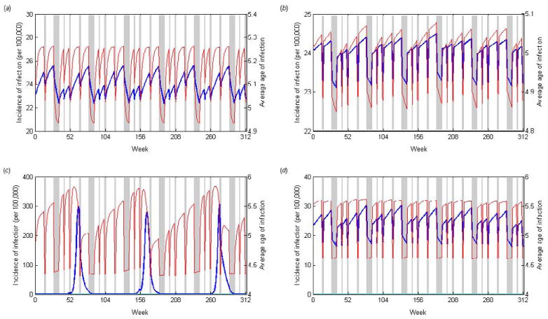
Age-structured model results using “term-time” seasonal forcing. The number of incident infections (blue lines) and the average age of first infection (red lines) are plotted over a six year period for (a) an acute infection (D = 1 week) assuming self-reported mixing, (b) a long duration infection (D = 12 weeks) assuming self-reported mixing, (c) an acute infection (D = 1 week) assuming RAS mixing, and (d) a long duration infection (D = 12 weeks) assuming RAS mixing. Holiday periods are represented by the gray shaded areas.
For RAS mixing, again the average age of infection tends to be higher during in-school periods and lower during vacation periods. However, when the duration of infectiousness is short (D = 1 week), there is a strong biennial cycle in the number of cases, such that there is a single epidemic peak occurring every other year just prior to the spring vacation period (Fig. 3c). As the duration of infectiousness increases, the biennial cycle becomes less prominent. Again the number of cases tends to increase during in-school periods and decrease during vacation periods such that the peak prevalence occurrs prior to the summer vacation period (Fig. 3d), and the lag time corresponding to the maximum correlation is approximately 0 weeks.
5. Age-structured SEIR model
A slight variation on the basic age-structured SIR model includes the addition of a latent period following infection of a susceptible individual, during which that person is not yet infectious to others; this is the SEIR (susceptible-exposed-infectious-recovered) model. We assume that the average duration of the latent period is one week, consistent with infections such as measles, rubella, and chickenpox (Anderson and May, 1991). The set of differential equations describing the system is as follows:
| (5.1) |
where λi is the same as defined for the SIR model. Again note that μS0 = ν and μE0 = μI0 = μR0 = 0. We use this SEIR model to examine how the addition of latent period prior to the onset of infectiousness affects the relationship between the number of cases and the average age of first infection.
The results of the SEIR model are similar to those of the SIR model (Table 3). The biggest discrepancy is that the lag time increases by 3 weeks (and ρ0 decreases) when we assume homogeneous mixing with D = 1 week. Furthermore, the predicted period of oscillations is no longer 2 years for acute infections; rather, there is a much weaker 1 year seasonal oscillation. This is consistent with what we would expect given the predicted period of intrinsic oscillations is given by T = 2π[A(D′ + D)]1/2, where (D′ + D) is the sum of the latent and infectious periods. When we exclude the latent period (D′ = 0) and assume D = 1 week and A = 5 years, the predicted period of oscillations is very close to 2 years, leading to resonance with the seasonal oscillations. However, when (D′ + D) = 2 weeks, the predicted period of oscillations is approximately 2.75 years and no resonant oscillations occur. The additional latent period has little or no effect on the relationship between the number of cases and the average age of infection under other population mixing assumptions.
Table 3.
Relationship between the number of cases and the average age of infection for the SEIR model.
| WAIFW | Outcome measure | Duration of infectiousness | |||
|---|---|---|---|---|---|
| 1 week | 4 weeks | 8 weeks | 12 weeks | ||
| Homogeneous | Lag time | 3 | 3 | 3 | 3 |
| ρ0 | 0.809 | 0.913 | 0.919 | 0.921 | |
| Amax - Amina | 0.005 | 0.006 | 0.004 | 0.004 | |
| Assortative | Lag time | 13 | 16 | 21 | 25 |
| ρ0 | -0.014 | -0.390 | -0.796 | -0.986 | |
| Amax - Amin | 0.096 | 0.146 | 0.064 | 0.039 | |
| Self-report | Lag time | 14 | 15 | 16 | 16 |
| ρ0 | -0.091 | -0.218 | -0.364 | -0.413 | |
| Amax - Amin | 0.066 | 0.102 | 0.058 | 0.041 | |
| RAS | Lag time | 40 | 42 | 41 | 40 |
| ρ0 | 0.173 | 0.290 | 0.232 | 0.162 | |
| Amax - Amin | 0.046 | 0.090 | 0.052 | 0.043 | |
Seasonal forcing = 5% for D=1week, 25% for D=4-12 weeks
6. Prevalent versus incident infections
Our primary analysis considers the relationship between the number of incident infections and the average age of such infections. Thus, our comparison to case notification data assumes that cases are reported at beginning of their infectious period or at a constant interval, e.g. 1 week, following the onset of infectiousness. Alternatively, one might assume that there is an equal probability of a case being reported at any point during the infectious period. If this is true, it would be more appropriate to model the relationship between the number of prevalent infections (Y) and the average age of prevalent infection (Ap). For acute infections, this discrepancy will be minimal, since the number of prevalent infections in a given week is approximately equal to the number of incident infections. However, for longer durations of infectiousness, our assumptions about whether incident or prevalent infections better represent case report data will likely impact the relationship between the number of cases and the average age of such cases. Thus, we evaluate the sensitivity of our results to this assumption.
For the basic SIR model assuming homogeneous mixing, the peak in the number of prevalent infections and the peak in the average age of prevalent infection occur at approximately the same time, i.e. l = 0 weeks for acute infections, but the lag time increases with longer durations of infectiousness (Table 4). When we assume population mixing is assortative or reflects self-reported patterns, again the lag time increases with increasing duration of infectiousness, and a duration of infectiousness of at least 4 weeks is required to obtain a negative correlation between incidence and mean age at lag 0 (Table 4). Again, it is possible to demonstrate mathematically that the results assuming homogeneous mixing are consistent with what we would expect (Appendix C).
Table 4.
Relationship between the number of prevalent infections (Y) and the average age of prevalent infection (Ap) for the basic SIR model.
| WAIFW | Outcome measure | Duration of infectiousness | |||
|---|---|---|---|---|---|
| 1 week | 4 weeks | 8 weeks | 12 weeks | ||
| Homogeneous | Lag time | 1b | 16 | 19 | 21 |
| ρ0 | 0.847 | -0.318 | -0.730 | -0.882 | |
| Amax - Amina | 0.072 | 0.038 | 0.058 | 0.068 | |
| Assortative | Lag time | 12 | 16 | 20 | 22 |
| ρ0 | 0.097 | -0.341 | -0.730 | -0.882 | |
| Amax - Amin | 0.240 | 0.229 | 0.121 | 0.097 | |
| Self-report | Lag time | 15b | 15 | 18 | 20 |
| ρ0 | 0.110 | -0.250 | -0.556 | -0.733 | |
| Amax - Amin | 0.946 | 0.169 | 0.116 | 0.105 | |
| RAS | Lag time | 40 | 40 | 26 | 24 |
| ρ0 | 0.083 | 0.081 | -0.985 | -0.967 | |
| Amax - Amin | 0.159 | 0.079 | 0.042 | 0.065 | |
Seasonal forcing = 5% for D = 1 week, 25% for D = 4-12 weeks
Epidemic period = 2 years
7. Discussion
We use seasonally-forced age-structured models to examine what aspects of the disease dynamics affect the relationship between the number of cases and the average age of first infection over the course of a single epidemic period. We explore a variety of parameter combinations and mixing assumptions, and find that the average age of first infection is greatest at or near the peak of the epidemic when we assume homogenous mixing regardless of the duration of infectiousness. When population mixing is at least partly assortative, or if we assume prevalent infections are more representative of case report data, the number of cases and average age of first infection become increasingly out of phase as the duration of infectiousness increases, such that when individuals are infectious for approximately 3 months or more, the average age of infection is lowest near the peak of the epidemic and greater during the trough, provided the seasonal forcing mechanism is not age-dependent. The degree of seasonal variation in the average age of infection is greatest for acute infections, particularly when mixing is non-homogeneous.
Theory derived from the long-term equilibrium dynamics of age-structured models suggests that the average age of infection should be inversely proportional to the incidence (Anderson and May, 1985). Higher incidence rates increase the likelihood of infection early in life, thereby leading to a lower average age of infection. Policies such as vaccination that decrease the incidence rate should increase the average age of infection in unvaccinated individuals (Anderson and May, 1983; Anderson and May, 1985; Anderson and May, 1991; Griffiths, 1973). Thus, the results of our model showing that the average age of infection is greatest at or soon after the seasonal peak in the number infected for acute infections may seem counter-intuitive. However, the long-term inverse relationship assumes that the system is in equilibrium, such that the proportion of each age class that is susceptible to infection remains constant, which is not the case for diseases exhibiting regular seasonal cycles.
Close inspection of the seasonal dynamics of the age-structured model assuming homogeneous mixing reveals that the amplitude of oscillations in the proportion susceptible is proportionally greater for the younger age classes than for the older age classes. As a result, those in the youngest age classes tend to experience the infection first, at the earliest stages of the epidemic. There is some epidemiologic evidence to support this in the case of influenza (Brownstein et al., 2005). As the epidemic progresses, there are relatively fewer susceptibles remaining in the youngest age classes, and therefore a slightly greater relative proportion of the cases occur among older individuals. This leads to an increase in the average age of infection, until the proportion susceptible among the older age classes has declined as well. The rate of replenishment of the susceptibles is greatest for the youngest age group since individuals are born into this age class at a constant rate. When the duration of infectiousness is short, the infection and recovery of most individuals in the youngest age groups occurs on a relatively quick time-scale, such that there is a considerable depletion of susceptibles by the time epidemic peaks; this leads to a noticeable change in the average age of first infection over the course of an epidemic. However, as the duration of infectiousness increases, the proportion susceptible declines more slowly and the amplitude of oscillations decreases; as a result, the degree of seasonal variation in the average age of infection is smaller.
If we assume that population mixing is at least somewhat assortative, then our models suggest that the peak in average age of infection is delayed somewhat relative to the peak in the epidemic. Again, the epidemic tends to be initiated by infections occurring among the youngest age group. However, since individuals are more likely to infect other members of their own age group, it takes longer for the transmission of infection to gradually spill over to older age groups.
When disease transmission is largely dependent upon high mixing rates among primary school-aged children, as in the RAS models, the epidemic tends to be initiated by the infection of these older children. Thus, the average age of infection tends to be greatest prior to the peak in the number of cases. However, in order to induce this relationship between the number of cases and the average age of infection, the mixing rate among school-aged children must be considerably greater than the mixing rate among younger children so as to compensate for the lower levels of susceptibility. Recent studies of mixing patterns (Mossong et al., 2008; Wallinga et al., 2006) suggest that if self-reported conversations are a good proxy for transmission-relevant contacts, then school-aged children should only have twice as many contacts as younger children, at most. Thus, in order for the contacts rates estimated for the RAS models to be applicable, the infection would have to be highly transmissible, such that transmission could occur over greater distances and would be more dependent upon factors such as classroom size than the number of conversational partners. This may be true for measles, but may not be as applicable to other respiratory or droplet-borne infections.
There is evidence suggesting that the average age of measles cases during the pre-vaccination era was greater during the first quarter of the year in which epidemics occurred than during the third quarter, when there were relatively few measles cases (Grenfell and Anderson, 1985). The authors pointed out that this seemed contrary to the intuition that the average age of cases should be lower during periods of high incidence, but they attributed it to age-related seasonal differences in mixing patterns. They argued that the majority of measles cases during epidemic periods occurred among school-aged children. During the non-epidemic summer months, school-aged children tended to have fewer contacts, but the mixing rate remained essentially the same for pre-school children, leading to a proportionally greater number of cases among these younger children (Grenfell and Anderson, 1985). While term-time forcing could generate this pattern, we show that their prior observation is in line with what might be expected for an acute immunizing infection such as measles even in the absence of term-time effects. Examination of pre-vaccination measles data on a weekly timescale may help distinguish whether or not term-time forcing is the primary determinant of changes in the average age of infection.
It is interesting to note that under the homogeneous mixing assumption, our results differ considerably for infections of longer duration depending on whether we assume incident or prevalent infections are more representative of the case report data. It is often assumed that the onset of symptoms and the onset of infectiousness occur at or around the same time. While this is true for most acute infections, for more chronic infections such as colonizing bacteria there will likely be more variability in the timing of symptoms and, more importantly, the timing of reporting in relation to the infectious period. Thus, it seems likely that the relationship between the number and age of reported cases will follow a pattern that lies somewhere between our results for incident and prevalent infections. Furthermore, this discrepancy is considerably less for other (perhaps more realistic) population mixing assumptions.
It remains to be seen whether it is possible to distinguish seasonal changes in the average age of infection due to the intrinsic dynamics from random variability in the case report data. Our results suggest that the degree of seasonal variation in the average age of first infection will be greatest for acute infections, which have a tendency to exhibit strong seasonal oscillations. For such infections, the change in the average age of first infection can be considerable when mixing is non-homogeneous (approximately 1 year in some cases, assuming conservatively that the amplitude of seasonal forcing is just 5% per year). However, for infections exhibiting weaker oscillations, seasonal changes in the age distribution of infection may be more difficult to detect. Assuming it is possible to distinguish seasonal variation in the average age of infection from case report data, our results suggest a number of ways in which this information may be useful in understanding the dynamics of infection and parameterizing models. For acute infections of known etiology, the relationship between seasonal changes in the number and mean age of cases may lend insight into the nature of population mixing. When population mixing is homogeneous, the average age of first infection tends to be greatest at or near the peak in the number of cases, while if mixing is at least partly assortative, the peak in the average age of infection tends to lag behind the peak in cases by two to three months. High rates of mixing in older age groups can reverse this pattern, such that the average age of infection is greatest prior to the peak in the number of cases as epidemics tend to begin among these older individuals. For infections of unknown etiology, such as Kawasaki disease, the analysis we present here suggests that the relationship between the number of cases and the average age of infection during seasonal oscillations in incidence is at least partly dependent upon the duration of infectiousness in a manner which is qualitatively insensitive to most realistic assumptions about population mixing behavior. Thus, examining the correlation between the number of cases and the average age of such cases may help to narrow down the search for an etiologic agent.
Acknowledgments
The authors thank Caroline Colijn for useful feedback in the analysis of the model, Megan Murray and Jamie Robins for constructive advice on the structure of this project, and David Burgner, Cecile Viboud, and Lone Simonsen for stimulating discussions that led to the worked described here. V.E.P. was supported by training grant T32 AI07535, and V.E.P. and M.L. were supported by cooperative agreement 5U01GM076497 (Models of Infectious Disease Agent Study) from the National Institutes of Health.
Appendix A. Proof of relationship between number and average age of incident infections
One way to verify the relationship between the average age of first infection (A) and the total number of cases (C) predicted by the model, and to show this relationship does not depend on the duration of infectiousness, is to examine the second derivative of A (d2A/dt2 = A″) at the peak of the epidemic. If A″ is negative at the peak of the epidemic, then this would indicate A is at or near its maximum, while if A″ is positive, there would be an inverse correlation between A and C at a lag of 0 weeks (ρ0 < 0).
Recall that is the total number of susceptible individuals and is the total number of prevalent infections at time t, and let be the weighted sum of the number of susceptibles in age group i at time t, where the weight ai is again the midpoint of age group i. Note that the average age of first infection at time t can be expressed as
| (A.1) |
The peak of the epidemic occurs when the number of incident cases ( for homogeneous mixing) reaches a maximum. This precedes the time when the number of prevalent infections (Y) is at a maximum by approximately the average duration of infectiousness (D), since incident cases will remain prevalent infections until they recover. Thus, at the peak of the epidemic, Y′ > 0 and Y″ < 0, where
| (A.2) |
and
| (A.3) |
Note that virtually everyone is recovered and immune by the time they reach the last age class (i = 80); thus, μI80 and μS80 ≈ 0. Therefore, since Y′ > 0, it follows from Eq. (A.2) that βX > δ. Given that Y″ < 0 at the peak of the epidemic, we can infer that at the peak, βν < β2XY − β′X.
The first derivative of A at the peak is given by
| (A.4) |
where
| (A.5) |
and
| (A.6) |
Therefore,
| (A.7) |
and the second derivative of A is
| (A.8) |
Note that neither A′ nor A″ depend on the duration of infectiousness, D.
Finally we prove that when Y″ < 0, the mean age of infection is at or near a maximum. Recall that Y″ < 0 implies βY(ν − βXY) − β′XY < 0. Furthermore, β′ ≤ 0 at this point since the peak in incidence occurs around the same time or slightly after the peak in the seasonal forcing parameter. Thus, βXY > ν when Y″ < 0. When the mean age of infection is peaking, A″ < 0, and therefore βXY > 2ν − μX/(A − 1). Note that when A′ = 0, ν − μX/(A − 1) = 0; thus, the conditions for A″ <0 and Y″ <0 are identical when the mean age of infection is at a maximum. This confirms our observation that the average age of first infection peaks at approximately the same time as the number of incident cases regardless of the duration of infectiousness.
Appendix B. WAIFW matrices
The WAIFW matrices described in Section 3 are as follows. All matrices are symmetric, such that βij = βji. Each matrix is scaled by a factor β0m, where m is the mixing type, such that the average age of infection is 4-6 years of age.
Homogeneous mixing:
Assortative mixing:
Self-reported mixing:
RAS mixing:
Appendix C. Proof of relationship between number and average age of prevalent infections
We can show that the relationship between the number and average age of prevalent infections is dependent on the duration of infectiousness, and that the average age of prevalent infections is greatest at or near the peak of the epidemic for acute infections by again examining the second derivatives.
Recall that is the total number of prevalent infections at time t, and let be the weighted sum of the number of infectious individuals in age group i at time t, where the weight ai is again the midpoint of age group i. Note that the average age of prevalent infection (Ap) at time t can be expressed as
| (B.1) |
The peak in the number of prevalent infections occurs when Y′ = 0 and Y″ < 0, where
| (B.2) |
given X = ΣSi, and
| (B.3) |
Again, virtually everyone is recovered and immune by the time they reach the last age class (i = 80), so μI80 and μS80 ≈ 0. Since Y′ = 0 at the peak of the epidemic, it follows from Eq. (B.2) that βX = δ. Also, Y″ < 0 at this point, so it follows from Eq. (B.3) that βν < β2XY − β′X.
Since Y′ = 0, the second derivative of Ap at the peak simplifies to
| (B.4) |
where
| (B.5) |
given Q = ΣaiSi, and
| (B.6) |
Therefore, substituting Eqs. (B.3) and (B.6) into Eq. (B.4) and recalling that βX = δ, we obtain
| (B.7) |
where again
| (B.8) |
is the average age of incident infections. Thus, Ap″ will be negative when βν(Ap − 1) > (β2XY − β′X + βX2δ)(Ap − A). Under homogeneous mixing, the difference Ap − A is approximately equal to the average duration of infectiousness measured in years, or μD. Since βν < β2XY − β′X, this will only occur when (Ap−A) is small, i.e. when the average duration of infectiousness is short.
Footnotes
Publisher's Disclaimer: This is a PDF file of an unedited manuscript that has been accepted for publication. As a service to our customers we are providing this early version of the manuscript. The manuscript will undergo copyediting, typesetting, and review of the resulting proof before it is published in its final citable form. Please note that during the production process errors may be discovered which could affect the content, and all legal disclaimers that apply to the journal pertain.
References
- Altizer S, Dobson A, Hosseini P, Hudson P, Pascual M, Rohani P. Seasonality and the dynamics of infectious diseases. Ecol Lett. 2006;9(4):467–484. doi: 10.1111/j.1461-0248.2005.00879.x. [DOI] [PubMed] [Google Scholar]
- Anderson RM, May RM. Vaccination against rubella and measles: quantitative investigations of different policies. J Hyg (Lond) 1983;90(2):259–325. doi: 10.1017/s002217240002893x. [DOI] [PMC free article] [PubMed] [Google Scholar]
- Anderson RM, May RM. Age-related changes in the rate of disease transmission: implications for the design of vaccination programmes. J Hyg (Lond) 1985;94(3):365–436. doi: 10.1017/s002217240006160x. [DOI] [PMC free article] [PubMed] [Google Scholar]
- Anderson RM, May RM. Infectious Diseases of Humans: Dynamics and Control. Oxford: Oxford University Press; 1991. [Google Scholar]
- Bolker BM, Grenfell BT. Chaos and biological complexity in measles dynamics. Proc Biol Sci. 1993;251(1330):75–81. doi: 10.1098/rspb.1993.0011. [DOI] [PubMed] [Google Scholar]
- Broutin H, Mantilla-Beniers NB, Simondon F, Aaby P, Grenfell BT, Guegan JF, Rohani P. Epidemiological impact of vaccination on the dynamics of two childhood diseases in rural Senegal. Microbes Infect. 2005;7(4):593–599. doi: 10.1016/j.micinf.2004.12.018. [DOI] [PubMed] [Google Scholar]
- Brownstein JS, Kleinman KP, Mandl KD. Identifying pediatric age groups for influenza vaccination using a real-time regional surveillance system. Am J Epidemiol. 2005;162(7):686–693. doi: 10.1093/aje/kwi257. [DOI] [PMC free article] [PubMed] [Google Scholar]
- Burgner D, Harnden A. Kawasaki disease: what is the epidemiology telling us about the etiology? Int J Infect Dis. 2005;9(4):185–194. doi: 10.1016/j.ijid.2005.03.002. [DOI] [PMC free article] [PubMed] [Google Scholar]
- Cannell JJ, Vieth R, Umhau JC, Holick MF, Grant WB, Madronich S, Garland CF, Giovannucci E. Epidemic influenza and vitamin D. Epidemiol Infect. 2006;134(6):1129–1140. doi: 10.1017/S0950268806007175. [DOI] [PMC free article] [PubMed] [Google Scholar]
- Dietz K. Transmission and control of arbovirus diseases. In: Ludwig D, Cooke KL, editors. Epidemiology. Philadephia: Society for Industrial and Applied Mathematics; 1975. pp. 104–121. [Google Scholar]
- Dietz K. The incidence of infectious diseases under the influence of seasonal fluctuations. In: Berger J, et al., editors. Lecture notes in biomathematics. Berlin, Germany: Springer; 1976. pp. 1–15. [Google Scholar]
- Dowell SF. Seasonal variation in host susceptibility and cycles of certain infectious diseases. Emerg Infect Dis. 2001;7(3):369–374. doi: 10.3201/eid0703.010301. [DOI] [PMC free article] [PubMed] [Google Scholar]
- Earn DJ, Rohani P, Bolker BM, Grenfell BT. A simple model for complex dynamical transitions in epidemics. Science. 2000;287(5453):667–670. doi: 10.1126/science.287.5453.667. [DOI] [PubMed] [Google Scholar]
- Earn DJ, Rohani P, Grenfell BT. Persistence, chaos and synchrony in ecology and epidemiology. Proc Biol Sci. 1998;265(1390):7–10. doi: 10.1098/rspb.1998.0256. [DOI] [PMC free article] [PubMed] [Google Scholar]
- Fales WT. The age distribution of whooping cough, measles, chicken pox, scarlet fever and diphtheria in various areas in the United States. American Journal of Hygiene. 1928;8:759–799. [Google Scholar]
- Fine PE, Clarkson JA. Measles in England and Wales--I: An analysis of factors underlying seasonal patterns. Int J Epidemiol. 1982;11(1):5–14. doi: 10.1093/ije/11.1.5. [DOI] [PubMed] [Google Scholar]
- Grassly NC, Fraser C. Seasonal infectious disease epidemiology. Proc Biol Sci. 2006;273(1600):2541–2550. doi: 10.1098/rspb.2006.3604. [DOI] [PMC free article] [PubMed] [Google Scholar]
- Grenfell BT, Anderson RM. The estimation of age-related rates of infection from case notifications and serological data. J Hyg (Lond) 1985;95(2):419–436. doi: 10.1017/s0022172400062859. [DOI] [PMC free article] [PubMed] [Google Scholar]
- Griffiths DA. The effect of measles vaccination on the incidence of measles in the community. J R Stat Soc, Series A. 1973;136(3):441–449. [Google Scholar]
- Griffiths DA. A catalytic model of infection for measles. Appl Statist. 1974;23(3):330–339. [Google Scholar]
- Lowen AC, Mubareka S, Steel J, Palese P. Influenza virus transmission is dependent on relative humidity and temperature. PLoS Pathog. 2007;3(10):1470–1476. doi: 10.1371/journal.ppat.0030151. [DOI] [PMC free article] [PubMed] [Google Scholar]
- Mossong J, Hens N, Jit M, Beutels P, Auranen K, Mikolajczyk R, Massari M, Salmaso S, Tomba GS, Wallinga J, Heijne J, Sadkowska-Todys M, Rosinska M, Edmunds WJ. Social contacts and mixing patterns relevant to the spread of infectious diseases. PLoS Med. 2008;5(3):e74. doi: 10.1371/journal.pmed.0050074. [DOI] [PMC free article] [PubMed] [Google Scholar]
- Olsen LF, Schaffer WM. Chaos versus noisy periodicity: alternative hypotheses for childhood epidemics. Science. 1990;249(4968):499–504. doi: 10.1126/science.2382131. [DOI] [PubMed] [Google Scholar]
- Rohani P, Earn DJ, Grenfell BT. Opposite patterns of synchrony in sympatric disease metapopulations. Science. 1999;286(5441):968–971. doi: 10.1126/science.286.5441.968. [DOI] [PubMed] [Google Scholar]
- Schenzle D. An age-structured model of pre- and post-vaccination measles transmission. IMA J Math Appl Med Biol. 1984;1(2):169–191. doi: 10.1093/imammb/1.2.169. [DOI] [PubMed] [Google Scholar]
- Snow RW, Marsh K. New insights inot the epidemiology of malaria relevant for disease control. British Medical Bulletin. 1998;54(2):293–309. doi: 10.1093/oxfordjournals.bmb.a011689. [DOI] [PubMed] [Google Scholar]
- Wallinga J, Teunis P, Kretzschmar M. Using data on social contacts to estimate age-specific transmission parameters for respiratory-spread infectious agents. Am J Epidemiol. 2006;164(10):936–944. doi: 10.1093/aje/kwj317. [DOI] [PubMed] [Google Scholar]
- Whitaker HJ, Farrington CP. Estimation of infectious disease parameters from serological survey data: the impact of regular epidemics. Stat Med. 2004;23(15):2429–2443. doi: 10.1002/sim.1819. [DOI] [PubMed] [Google Scholar]