

Abstract
Entrainment, where oscillators synchronize to an external signal, is ubiquitous in nature. The transient time leading to entrainment plays a major role in many biological processes. Our goal is to unveil the specific dynamics that leads to fast entrainment. By studying a generic model, we characterize the transient time to entrainment and show how it is governed by two basic properties of an oscillator: the radial relaxation time and the phase velocity distribution around the limit cycle. Those two basic properties are inherent in every oscillator. This concept can be applied to many biological systems to predict the average transient time to entrainment or to infer properties of the underlying oscillator from the observed transients. We found that both a sinusoidal oscillator with fast radial relaxation and a spike-like oscillator with slow radial relaxation give rise to fast entrainment. As an example, we discuss the jet-lag experiments in the mammalian circadian pacemaker.
Introduction
Biological rhythms are ubiquitous in nature and are found in diverse systems, from spiking neurons to animal populations with periods ranging from milliseconds to years. Our everyday life exhibits many behavioral and physiological oscillations that interact with the external fluctuating environment. Biological pacemakers typically interact with other oscillators including for example coupled rhythms of heart, respiration and movement [1], vocal fold oscillations [2] and singing duets of birds [3]. These interactions can lead to mutual synchronization as in the collective blinking of fireflies [4] and entrainment in which oscillators synchronize to a common signal. An example of this is the left and right birdsong control nuclei HVc that show synchronization in the absence of interhemispheric connections [5]. Another example is the entrainment of plant-leafs movements to the light-dark and cold-warm cycles [6]. Complex interactions between multiple oscillators are observed in the mammalian suprachiasmatic nucleus (SCN), where mutual synchronization and entrainment are combined. These tiny nuclei situated in the anterior hypothalamus are responsible for controlling endogenous circadian rhythms. Many different body functions like sleep-wake cycles and body temperature rhythms are regulated by centrally generated neuronal and hormonal activities. The SCN consists of two nuclei of about ten thousand densely packed neurons and generates a stable robust period of about 24 h. The SCN has the striking ability of fast reentrainment as observed in jet-lag type experiments, where after an abrupt phase shift of 6 h, the SCN can be almost completely reentrained within one cycle [7]–[9]. Also from the induced loss of rhythmicity in SCN slices after application of tetrodotoxin (TTX, a voltage gated sodium channel blocker), the SCN cells resynchronize within one cycle [10]. When TTX is applied, the oscillations are lost at a single cell level but after washing TTX out, the cells start oscillating again in a synchronized manner after 1 day. Such short transients times are remarkable, bearing in mind the large number of coupled oscillators involved and the diversity of their initial conditions and periods [11], [12]. How synchronization and entrainment mechanisms work within the SCN neurons is one of the main open problems in the field of circadian rhythms. Furthermore, in jet-lag and shift work schedules, the reentrainment time is of major relevance and has been associated to a number of diseases, ranging from sleep disorders to cancer [13]–[15].
Several mathematical models of SCN cells have been proposed with an increasing complexity (using 7 up to 73 differential equations [16]–[18]), none of which describes the short reentrainment times in detail. Our goal in this present paper is to unveil the specific dynamics that can lead to ultrafast entrainment. We present a generic model to characterize transient times leading to entrainment. This model is governed by two basic properties of the oscillator: (a) the radial relaxation timescale and (b) the phase velocity distribution around the limit cycle. When an oscillator is perturbed, the radial relaxation timescale determines the rate of convergence back to the unperturbed amplitude and it can hence be associated with robustness towards amplitude fluctuations. The phase velocity distribution determines the waveform of the oscillation.
Studying the transient time as a function of these two properties will give us a general understanding of how fast can entrainment be reached. Those two basic properties are inherent in every oscillator and, therefore, such a concept can be applied to many biological systems to predict the transient time to entrainment. Even more interestingly, one can infer properties of the underlying oscillator from the observed transient times as we will show later. Helpful insights derived from transients of an oscillatory system have already been applied in heart cells studies [19]. Although we focus on biological applications, the presented theory can be applied to many other oscillatory systems undergoing entrainment.
Results
Timescales of entrainment
When a system is entrained, it reaches a stable phase relation with the external rhythm and thus their phase difference becomes constant (see Materials and Methods). The transient time it takes to reach this stable phase relation depends on the initial conditions (ICs), the entrainment signal and the properties of the oscillator. An example of these transients for a generic circadian oscillator is shown in Figure 1. Each initial condition has an associated initial phase (see gray dots in Figure 1B and C), different initial phases can lead to big differences in the transient time to entrainment. Figure 1A shows the time evolution of two initial conditions,  and
and  , leading to a long transient (pink) and a short transient (blue) respectively. This can also be observed in a phase evolution plot where
  needs 8 days to achieve a stable phase relation whereas
  only 1 day (see Figure 1B). The dependence on initial conditions for a specific circadian oscillator model has already been studied [20]. A self-sustained oscillator is able to entrain just to certain combinations of entrainment amplitudes and periods that define the so-called entrainment region or 1∶1 “Arnold tongue” (see Figure 1D). In other words, each entrainment amplitude entrains the system within a certain period range, from a minimum
  to a maximum
  entrainment period, known as range of entrainment. Typically, at the borders of this entrainment region the transients leading to entrainment are much longer than those at the center (see Figure 1E). In the following we focus on those inherent properties of the oscillator that determine the transients.
Figure 1. Basic mechanisms involved in the entrainment of an oscillator.

(A) Time series for two initial conditions, ICslow and ICfast, leading to a long transient (pink) and a short transient (blue), respectively. The green bars represent the entrainment signal. (B) Phase evolution for both initial conditions. ICfast entrain after 1 day while IC slow needs 8 days (fig. 1) (C) Oscillator limit cycle representation with 24 marked initial conditions (gray). (D) Schematic representation of the entrainment region as a function of the entrainment amplitude and period (often termed 1∶1 “Arnold tongue”). Gray scale represents different transients to entrainment zones within the entrainment region. The green dots represent the section of the entrainment region (entrainment range) for a certain entrainment amplitude and in (E) their associated entrainment times are plotted as a function of the entrainment period. Computational details of A,B and E are given in Materials and Methods.
Generic oscillator model
As will be seen, our results indicate that two characteristics of the oscillator determine the transients: the radial relaxation time and the phase velocity around the limit cycle. To better illustrate the dependence of transient times on these two properties, we introduce a simple model oscillator that can mimic various oscillators. We use a generic circular oscillator of radius 1 and period 1 (arbitrary units) so the results can be easily rescaled to other systems. As a specific model, we introduce a variation of the Poincaré oscillator [21], given by
| (1) |
| (2) |
This oscillator can be smoothly switched from a sinusoidal shape to a spike-like oscillator, while the radial relaxation can be independently controlled (see Figure 2). Equation 1 describes the radial evolution and has a stable orbit at  , with a radial relaxation controlled by the parameters
  and
and  . For
. For  the radial relaxation is exponential and for
  the radial relaxation is nonlinear. For
  the radial relaxation time,
  , is long and for
  the radial relaxation time is short, sometimes referred to as “sloppy” and “rigid” oscillators respectively (see Figure 2E and F). Equation 2 describes the phase evolution or, in other words, the velocity around the limit cycle, where
  controls the velocity difference between the fastest (
 ) and slowest (
 ) points. The “offset” is a small positive constant and guarantees that the velocity is never zero (
 ). For
  (i.e.,
  ), there are no velocity variations along the limit cycle, and the oscillator is sinusoidal (see Figure 2A and B). For
  , we have large velocity differences along the limit cycle, leading to a spike-like behavior (see Figure 2C and D).
Figure 2. Limit cycle representations in phase space for a sinusoidal and spike-like oscillator together with their time series.

(A) Sinusoidal oscillator: limit cycle with 12 marked phase points (dots) and isochrons (rays). The intersection of each isochron with the limit cycle determines the phase. (B) Temporal evolution of  variable with parameters
  . (C) Spike-like oscillator, where most isochrons are concentrated in a small region of the limit cycle. (D) Temporal evolution of the
  variable with parameters
  . Representations of both oscillators (sinusoidal or spike-like) with short radial relaxation time (E) and long radial relaxation time (F) are also shown. Computational details are given in Materials and Methods.
We use this generic limit cycle model instead of the widely used phase models because amplitude dynamics will be of fundamental importance in characterizing transients leading to entrainment. The phase velocity around the limit cycle determines the temporal shape of the oscillation (waveform), as illustrated in Figure 2B and D. The radial relaxation rate  together with the degree of nonlinearity controlled by the parameter
  determines the timescale of convergence of perturbed solutions to the limit cycle (see Figure 2E and F). It can be associated with robustness towards amplitude fluctuations.
This oscillator, a modified Poincaré oscillator [21], belongs to the class of radial isochron limit cycles (RILC) due to its radial symmetry (see Materials and Methods). Many examples of useful biological insights based on RILC's can be found elsewhere [1], [21], [22]. Here we use the Winfree definition of isochrons as lines in phase space leading to the same asymptotic phase. Thus all initial conditions located on the same isochron will reach the limit cycle with the same phase [23]. The intersections of the isochrons and the limit cycle trajectory are the temporal phase points (see the dots in Figure 2A and C). In the case of RILCs, the isochron structure in the whole phase space can be deduced from the distribution of temporal phases. Thus a sinusoidal oscillator has equally distributed phase points and isochrons (see Figure 2A). A spike-like oscillator, on the other hand, makes a rapid excursion along the fast branch to spend most of its time at the slow branch. This time scale separation generates an asymmetric distribution of isochrons at the limit cycle by compressing them around the slow branch (see Figure 2C). The isochron distribution will be essential for the general understanding of the transient time to entrainment. As mentioned, our model was designed such that the phase velocity around the limit cycle and the radial relaxation time can be independently controlled to explore their influence on transients. For clarity, the oscillator will be rescaled to a period of 1 day and entrained with pulse-like perturbations of 1 h length. Square waveform oscillators, like the van der Pol oscillator in the relaxation regime, are not captured by this  . In order to simulate square waveform oscillators a new
  is introduced (see Figure S1 in Supporting Information).
Median time to entrainment
The time to entrainment depends strongly on the period ratio of external and internal rhythms (detuning) and on the initial phase (ICs). The internal period, such as the free-running period in circadian biology, and phase of the oscillators are typically unknown or difficult to measure. Therefore, we minimize the effects of detuning and initial conditions by studying ensembles of different external periods and initial phases. This allow us to associate a characteristic  with specific properties of an oscillator. The median time to entrainment
  is the median value of 12 different
  s. We use 12 different external periods evenly distributed within the range of entrainment to calculate the median as shown in Figure 1D and E. Additionally, for each external period,
  is taken as the median time from 24 uniformly distributed initial temporal phases (see Figure 1D). By taking both medians, we reduce the dependence on initial condition and entrainment period significantly (see Materials and Methods).
We start our results discussion with the exponential radial relaxation case ( in Equation 1) and describe the nonlinear case at the end of this section. For the case of exponential relaxation, we calculate the time to entrainment
  for different oscillator types using a broad range of values of phase velocity parameters
  and of radial relaxation rates
  , such that
  shows significant variations (see Figure 3). The entrainment signal was generated with short and medium-sized square periodic pulses. Specifically, we used 1 h pulse length with an amplitude of 0.8. This leads to a “range of entrainment” similar to that observed in rat locomotor activity under light pulse entrainment
  [24]. As mentioned above, the “range of entrainment” refers to the range of periods that a self-sustained oscillator is capable of entraining by a 1∶1 frequency ratio.
Figure 3. Median times to entrainment  as a function of the phase velocity distribution around the limit cycle
  and the radial relaxation constant
  .
.

Gray scale encodes the time to entrainment where black represents long  and white represents short
  . Both axes are plotted on logarithmic scales and
  in Equation 1. Computational details are given in the Materials and Methods.
According to Figure 3, the longest time to entrainment is found when the limit cycle has a sinusoidal temporal pattern and if the radial relaxation time is long (box 1 in Figure 3). The radial relaxation time,  , is in this case much longer than all other involved time scales: external periods
  , endogenous period (24 h) and pulse duration (1 h). Such long radial relaxation times allow the entrainment pulses to considerably perturb the trajectory of the limit cycle, leading to an expanded entrained orbit (a representative scheme of the mechanism is shown in Figure 4). Between the pulses, however, the system has not enough time to relax back to the original unperturbed orbit. A sinusoidal oscillator (
 ) implies equally distributed isochrons along the limit cycle and thus all isochrons diverge symmetrically from the limit cycle center. While the limit cycle expands, the isochrons spread apart, so phase changes induced by the same pulse size decrease. The phase change induced by a single pulse can be deduced from the difference between the starting isochron, where the perturbation starts, and the final isochron, where the trajectory is located after a given perturbation (see pink arrows in Figure 4). The combination of limit cycle expansion and equally distributed isochrons reduces the effect of each pulse. Very few isochrons are crossed leading to smaller phase changes per pulse. Consequently, it a rather long time to reach the final stable phase. For illustrative purposes we use vertical pulses in Figure 4, but similar features are observed with other types of entrainment signals.
Figure 4. Representative sinusoidal and spike-like limit cycles with long radial relaxation time.

Isochrons are represented as thin rays and perturbation pulses as pink arrows. (A) Unperturbed sinusoidal limit cycle trajectory (dashed small circle) and the expanded entrained limit cycle (solid large circle) for the sinusoidal oscillator. Initially the pulse generates a phase change up to 4 h, but later the pulse phase shift is reduced to less than 0.5 h. (B) Unperturbed spike-like limit cycle trajectory (dashed small circle) and the expanded entrained limit cycle (solid big circle) for the spike-like oscillator. Initially the pulse generates phase advances up to 14 h and, after some pulses, the phase shifts are still 8 h. The original limit cycle ( ) expands here about 7 times. The lower panels show the characteristic time series pattern of a sinusoidal and spike-like oscillator.
Surprisingly, the median time to entrainment  can be reduced up to 12-fold in our parameter range by changing independently
  or
or  . Keeping
  but increasing
  smoothly, changes the sinusoidal waveform oscillator into a spike waveform oscillator (see box 4 in Figure 3). The spike-like oscillator is also known as relaxation oscillator due to its fast and slow branches. The oscillator spends most of its time on the slow branch, so most stimuli are received on this branch. Spike-like oscillators have lower isochron divergence angles from the origin (see Figure 4B). This small isochron divergence allows considerable phase shifts of pulses despite the expansion of the limit cycle. This isochron clustering and, consequently, their low divergence angles allow the system to reach the final stable phase much faster.
As shown in Figure 3, an increase in the relaxation rate  leads to a drastic reduction in the median transient time
  as well. In this case, the radial relaxation time is much shorter than the period keeping the trajectory to the unperturbed limit cycle with keeping the trajectory to the unperturbed limit cycle with
  . Thus pulses induce considerable phase shifts for every given pulse and phase shifts are not reduced due to limit cycle expansion (compare box 2 in Figure 3).
The spike-like oscillator with short radial relaxation time is optimal as far as time to entrainment is concerned, because isochrons are concentrated in the slow branch without suffering from limit cycle expansion (see box 3 in Figure 3). In this case, perturbations induce large phase jumps, leading quickly to a stable phase from almost any initial condition.
In the present example, we used entrainment pulse amplitudes of 0.8, but qualitatively similar results are also observed with smaller amplitudes and also with sinusoidal perturbations (see Figure S2 in Supporting Information). As shown in Figure S2, the entrainment signal amplitude and waveform do not play a major role in determining the transient to entrainment.
Oscillators with highly nonlinear radial relaxation exhibit a much shorter median time to entrainment  as shown in Figure S2C and D in Supporting Information. This property is captured by our model using
  in Equation 1. The normal form of limit cycles arising via supercritical Hopf bifurcations corresponds to
  . Due to this strong nonlinearity, perturbations to the limit cycle trajectory relax rapidly back to the unperturbed limit cycle reducing considerably the limit cycle expansion effect (see Figure S2D). In the following, we relate our theory to a specific biological rhythm to gain insight into the properties of the system.
Fast entrainment in the mammalian circadian pacemaker
Physiological and behavioral processes in most organisms are synchronized with a 24 h day-night rhythm. Mammals have a central pacemaker located in the hypothalamic suprachiasmatic nucleus (SCN) that orchestrates circadian rhythms for the whole body. The SCN consists of two nuclei of about ten thousand densely packed neurons and generates a stable robust period of circa 24 h. This stable neuronal and hormonal rhythm regulates many different body functions. Cells within the SCN have an endogenous molecular clock based on a network of interlocking feedback loops of genes and proteins. The intercellular coupling between individual neurons generates not only a robust 24 h collective self-sustained rhythm under constant conditions (complete darkness) but also confers robustness against mutations [25]. The suprachiasmatic nucleus has a heterogeneous complex architecture. There is spatial heterogeneity, and individual neurons differ in their neuropeptide expression, light responsiveness, phase, and free running period [11], [12], [26]. For example, individual periods of dispersed cells span over 20 to 30.9 h with an average period of  . In organotypic slice cultures, periods range from 22.4 to 26.7 h with an average of
  [12]. Surprisingly, despite this complexity, the SCN exhibits fast reentrainment. In jet-lag type experiments the SCN can be almost completely reentrained within one day after an abrupt phase shift of 6 h [7]–[9]. Advanced microscopic techniques allow single cell bioluminescence measurements of clock proteins at intervals as short as 20 min. These measurements display almost sinusoidal oscillations [10], [25]. However, bioluminescence measurements provide only smoothed time series of specific reporter constructs and thus it is not entirely clear how sinusoidal the underlying core oscillator is. From our generic model, we predict that the observed fast reentrainment can be achieved in the following ways: (i) Sinusoidal waveform oscillator with relative short radial relaxation times (box 2 in Figure 3); (ii) spike-like oscillations with long relaxation time (box 4 in Figure 3); or (iii) a spike-like waveform and short radial relaxation time (box 3 in Figure 3). If SCN cells are self-sustained sinusoidal oscillators, we predict that the SCN cell oscillators have a short radial relaxation time. The radial relaxation time can be experimentally determined via a nonlinear fit to a time series in which an amplitude relaxation can be observed as in Figure 1A. The nonlinear fit can be done with the ansatz
 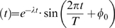 , where
  is time,
  is the oscillation period,
  the initial phase difference and
  is the radial relaxation from which the radial relaxation time
  can be directly obtained. In the vicinity of the limit cycle, the radial relaxation rate can be directly connected to the Floquet exponents. Large Floquet exponents (short radial relaxation times) have already been predicted on the basis of robustness studies using different clock models [27] and by optimizing a specific feedback model [28]. Our generic approach is based on one single characteristic, namely, the transient time to entrainment, and thus our prediction is independent of specific model assumptions. Most SCN cell models assume self-sustained oscillation, but experimental data [29], [30] and theoretical predictions [31], [32] suggest an alternative scenario, where most SCN cells might behave as damped oscillators. Detailed characterization of the transient time to entrainment with a mixture of sustained and damped oscillators is beyond the scope of the present work.
The Goodwin oscillator
The Goodwin oscillator [33] is a minimal model that describes the oscillatory negative feedback regulation of a protein which inhibits its own transcription. It provides a basic description of the central components in the circadian oscillators of Neurospora, Drosophila, and mammals [31], [34]. In this model, a clock gene mRNA ( ) produces a clock protein (
 ) which, in turn, activates a transcriptional inhibitor (
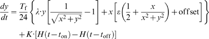
 ). Here we study a version of the Goodwin oscillator successfully used to model data from dermal fibroblasts from skin biopsies of human subjects [35]. The aim of that study was to investigate whether different types of behavior, early (“larks”) or late chronotypes (“owls”), have different clock properties in dermal fibroblasts. The model equations are:
| (3) |
| (4) |
| (5) |
This model describes the time evolution of mRNA ( ), of a cytosolic clock protein (
 ) and a nuclear clock protein (
 ). Concentrations of these are measured in arbitrary units (a.u.). This model has mostly linear kinetics with production rate constants
  and
and  and degradation rate constants
  ,
,  , and
, and  , all rate constants in
  . The Hill function, which expresses the transcription rate that is inhibited by the nuclear clock protein (
 ), has a maximal rate
  a.u./h, a half-saturation point
  a.u., and a Hill coefficient which we vary between
  and
and  . Our aim is to compare our generic predictions discussed above with a biochemical oscillator model. All eight parameters have an influence on the dynamics of the system. It has been shown that the Hill coefficient has a strong influence on the oscillator properties [35]. Therefore, we choose the Hill coefficient as the parameter to calculate the associated time to entrainment
  . Indeed, simulations confirm that the Hill coefficient has a strong effect on the time to entrainment. In Figure 5A, an increase from
  to
to  reduces the time to entrainment 5-fold. The entrainment signal was applied to all three dynamical variables in turn: to the cytosolic protein concentration, to mRNA concentration and to nuclear protein concentration. We observe qualitatively similar results in all three cases. Furthermore, in order to relate these transient times to our generic models, we extract for each Hill coefficient in the Goodwin model the velocity variations along the limit cycle parameter
  and the Floquet exponent associated with the radial relaxation timescale parameter
  . In this way, we can project these values on our plots for three models of radial oscillators (see Figure 5B, C and D). Interestingly, the Hill coefficient changes both velocity variations along the limit cycle
  and the radial relaxation timescale
  . Importantly, these two parameters govern the transients also in this higher-dimensional biochemical model. This is a demonstration that biochemical models are amaneable for studies using the concept developed in this paper.
Figure 5. Median time to entrainment  for the Goodwin model and the comparison with three radial oscillators models.

(A) Median time to entrainment for the Goodwin oscillator as a function of the Hill coefficient.  was calculated for an entrainment signal applied separately to each variable: the cytosolic protein concentration (pink), the mRNA concentration (dark violet) and the nuclear protein concentration (brown). (B)
  for a linear oscillator and the values of
  and
and  extracted from the Goodwin oscillator (green). (C)
  for a Poincaré oscillator and the values of
  and
and  extracted from the Goodwin oscillator (green). (D)
  for a Hopf-like oscillator and the values of
  and
and  extracted from the Goodwin oscillator (green).
  was calculated as in Figure 3 with relative pulse strength 0.4.s.
In addition to the results presented above we also checked if our findings hold for square-waveform oscillators, alternative entrainment signals and the more general scenario of mutually coupled oscillators (see Figures S1, S2 and S3 in Supporting Information). In all three cases we obtained qualitatively similar results in agreement with our concept.
Discussion
To our knowledge, ours is the first study that characterizes the transient time to entrainment in terms of the oscillator properties. Entrainment can be regarded as a particular case of synchronization with unidirectional coupling between the oscillators. Therefore, similar features observed in our results might be expected in other synchronization scenarios (see Supporting Information S1). The time to synchronization for a network of oscillators has been studied for several systems using analytical approaches [36]–[40] and numerical simulations [41]–[43]. Most synchronization studies focused on specific model oscillators at the network level and derived scaling laws associated with the number of oscillators. In [41] and [43], the synchronization rate of different conductance based models (Hodgkin-Huxley type models) was studied. Both studies showed that, a spike-like oscillator reached a synchronized state much more rapidly than a sinusoidal oscillator. Interestingly, it has been shown that synchronization can be achieved in a few cycles by relaxation oscillators [44] and by more sinusoidal “repressilators” [45]. Generally in models, the radial relaxation time and the phase velocity cannot be controlled independently. Therefore, changing the waveform pattern generally also changes the radial relaxation time, compounding the contributions of both properties and confusing the interpretation. Indeed, we observed this in the case of the Goodwin oscillator while increasing the Hill coefficient (see Figure 4C). Our goal was to reach a general understanding of the transient to entrainment based on topological representations. We use numerical simulations to exemplify our basic ideas. The model independent results can be related to most previously conducted studies.
Under the assumption that SCN cells are self-sustained sinusoidal oscillators, we predict that single cell oscillators have a short radial relaxation time. However, we cannot exclude that some SCN cells are spike-like oscillators and exhibit short transients this way. In fact, each SCN cell is a complex molecular oscillator and certain variables might exhibit a sinusoidal shape while others might have a spike-like shape. Perhaps, the pathway governing transients might be associated with a spike-like components. Time scale separations that support this view can be inferred from the rapid reentrainment observed in the SCN. Experiments with light pulses show that some core components of the SCN are able to respond to light within 1 h [46], [47].
In summary, we have shown how the time to entrainment is governed by the interplay of the radial relaxation time and the phase velocity distribution around the limit cycle. The time to entrainment  might be considered as an essential dynamical feature of an oscillator. In many systems, this quantity can be more easily extracted from experimental data than other related dynamical features such as Floquet exponents or isochron distributions. The median transient time to entrainment can be used to infer properties of the underlying oscillator from the observed transient times.
Materials and Methods
Model oscillator
The oscillator was designed to explore how the median time to entrainment  depends on a few generic parameters that are applicable to a big class of oscillators. In Equation 2,
  describes the phase evolution, where the parameter
  controls the ratio between the slowest and fastest velocities around the limit cycle. For
  ,
,  results in a sinusoidal oscillation (dashed blue line in Figure 6), for
  , a spike-like oscillation is generated (black line in Figure 6) and for a new
  we obtain a square-waveform oscillator (pink curve in Figure 6). The parameter
  controls the radial relaxation time independently of the phase dynamics. In the vicinity of the limit cycle,
  can be associated with the Floquet exponents, and
  with the isochron structure [23] of the limit cycle. This model allows us to create a spike-like oscillator with arbitrary Floquet exponents.
Figure 6. Phase velocity  as a function of the phase for different
  .
.

 controls the velocity gap between the fastest and slowest points and the parameter “offset” guarantees that the velocity is never zero. The black line corresponds to a spike-like oscillator, the pink line corresponds to the square-waveform oscillator and the dashed blue line corresponds to a sinusoidal oscillator with a constant phase velocity around the limit cycle.
A modified Poincaré oscillator is also known as radial isochron limit cycle due to the radial structure of its isochrons. The phase dynamics  is independent of the radial variable
  . Isochrons can be analytically calculated in some simple cases [21] or otherwise extracted with numerical approaches [48], but these approaches are not needed here since the isochrons can be projected directly from the temporal phase points plotted in Figure 3. Isochrons are a powerful tool to understand the phase changes induced by perturbations [49].
The simulations were carried out using the equations 1 and 2 with  and in Cartesian coordinates:
| (6) |
 |
(7) |
Here  , the unscaled period, depends on the parameters
  and offset. As discussed below we rescaled the period to 24 h by choosing an appropriate scaling factor
  . The entrainment signal
  is the Heaviside step function,
  is the pulse strength, the pulse start time is
  , with
  the entrainment period,
  and
and  is the pulse end time.
Time to entrainment
Our numerical experiments were designed to reduce dependencies on initial conditions and entrainment frequency. In Figure 3 we calculated the  for a wide range of
  and
and  values. Each point of the plot was calculated following the same numerical protocol: 1) Choose a parameter combination (
 ) of interest and rescale the system to a period
  h. 2) Calculate the range of entrainment and choose entrainment frequencies equidistributed within this range. 3) Choose initial temporal phases
  . The 24 h temporal initial phases are located around the unperturbed limit cycle (gray dots in Figure 1B and C), i.e. each initial condition is given by
 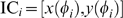 , where
  with
with  . 4) Start the simulations with periodic 1 h vertical pulses and calculate the instantaneous phase difference between the oscillator and the train of pulses for a total duration of 500 days (see Figure 1B). 5) The time to entrainment is considered to be reached if the mean phase difference of eight consecutive cycles is smaller than 5 minutes. Otherwise, no entrainment is detected. 6) Repeat steps 3–5 for the 24 different temporal phase initial conditions and then take their median value Te (see Figure 1C). 7) Repeat steps 2–6 for 12 evenly distributed frequencies within the total range of entrainment and then take their median value
  (see Figure 1E). 8) Choose another combination of
  and
and  and restart the protocol.
Supporting Information
(0.06 MB PDF)
Square waveform oscillator, its time series and the median time to entrainment. (A) Square waveform oscillator: limit cycle with 24 marked phase points (dots) and isochrons (rays). The intersection of each isochron with the limit cycle determines the phase and (B) the temporal evolution of x variable with parameters ε = 1, offset = 0.02, n = 0 and (C) the median time to entrainment <Te> as a function of the phase velocity around the limit cycle, ε, and radial relaxation constant, λ, for pulse entrainment. Gray scales refer to the median time to entrainment, where black represents long and white short <Te>.
(0.72 MB TIF)
Median time to entrainment <Te> for different entrainment signals and oscillators, under soft-pulses entrainment and under medium-sized-pulses for a nonlinear oscillator and for a Hopf oscillator. (A) Entrainment under sinusoidal perturbations with amplitude 0.05. (B) Entrainment under pulse perturbation with amplitude 0.4. (C) Entrainment under 1 h pulse perturbation with amplitude 0.8 for a nonlinear radial relaxation oscillator. (D) Entrainment under 1 h pulse perturbation with amplitude 0.8 for a Hopf oscillator. The median time to entrainment is plotted as a function of the phase velocity around the limit cycle, ε, and radial relaxation constant, λ. Gray scales refer to the median time to entrainment, where black represents long and white short <Te>. Both axes are plotted using logarithmic scales.}
(1.23 MB TIF)
Time to synchronization for two coupled oscillators. (A) Time to synchronization of two coupled “sloppy’ oscillators as a function of their transition from sinusoidal to a spike-like oscillator (B) Time to synchronization of two sinusoidal oscillators as a function of their transition from “sloppy’ to “rigid’ oscillator. See Supporting Information for model details.}
(0.83 MB TIF)
Acknowledgments
We thank Pål Westermark, Arkady Pikovsky and Achim Kramer for stimulating discussions and Anmar Khadra and Manuela Benary for carefully reading the manuscript.
Footnotes
Competing Interests: The authors have declared that no competing interests exist.
Funding: This work was supported by the Deutsche Forschungsgemeinschaft (SFB 618) and the EU-network Biosimulation. http://www.biologie.hu-berlin.de/forschung/SFB_618/ and http://biosim-network.eu/biosimulation_/ The funders had no role in study design, data collection and analysis, decision to publish, or preparation of the manuscript.
References
- 1.Glass L, Mackey MM. Princeton University Press; 1988. From Clocks to Chaos: The Rhythms of Life. [Google Scholar]
- 2.Herzel H, Berry D, Titze I, Steinecke I. Nonlinear dynamics of the voice: Signal analysis and biomechanical modeling. Chaos. 1995;5:30–34. doi: 10.1063/1.166078. [DOI] [PubMed] [Google Scholar]
- 3.Laje R, Mindlin GB. Highly structured duets in the song of the south american hornero. Phys Rev Lett. 2003;91:258104. doi: 10.1103/PhysRevLett.91.258104. [DOI] [PubMed] [Google Scholar]
- 4.Greenfield M, Tourtellot M, Snedden W. Precedence effects and the evolution of chorusing. Proc Roy Soc Lond B. 1997;264:1355–1361. [Google Scholar]
- 5.Schmidt MF. Pattern of interhemispheric synchronization in hvc during singing correlates with key transitions in the song pattern. J Neurophysiol. 2003;90:3931–3949. doi: 10.1152/jn.00003.2003. [DOI] [PubMed] [Google Scholar]
- 6.Millar AJ. Input signals to the plant circadian clock. J Exp Bot. 2004;55:277–283. doi: 10.1093/jxb/erh034. [DOI] [PubMed] [Google Scholar]
- 7.Yamazaki S, Numano R, Abe M, Hida A, Takahashi R, et al. Resetting central and peripheral circadian oscillators in transgenic rats. Science. 2000;288:682–685. doi: 10.1126/science.288.5466.682. [DOI] [PubMed] [Google Scholar]
- 8.Nagano M, Adachi A, Nakahama K, Nakamura T, Tamada M, et al. An abrupt shift in the day/night cycle causes desynchrony in the mammalian circadian center. J Neurosci. 2003;23:6141–6151. doi: 10.1523/JNEUROSCI.23-14-06141.2003. [DOI] [PMC free article] [PubMed] [Google Scholar]
- 9.Nakamura W, Yamazaki S, Takasu NN, Mishima K, Block GD. Differential response of period 1 expression within the suprachiasmatic nucleus. J Neurosci. 2005;25:5481–5487. doi: 10.1523/JNEUROSCI.0889-05.2005. [DOI] [PMC free article] [PubMed] [Google Scholar]
- 10.Yamaguchi S, Isejima H, Matsuo T, Okura R, Yagita K, et al. Synchronization of cellular clocks in the suprachiasmatic nucleus. Science. 2003;302:1408–1412. doi: 10.1126/science.1089287. [DOI] [PubMed] [Google Scholar]
- 11.Welsh DK, Logothetis DE, Meister M, Reppert SM. Individual neurons dissociated from rat suprachiasmatic nucleus express independently phased circadian firing rhythms. Neuron. 1995;14:697–706. doi: 10.1016/0896-6273(95)90214-7. [DOI] [PubMed] [Google Scholar]
- 12.Honma S, Nakamura W, Shirakawa T, Honma K. Diversity in the circadian periods of single neurons of the rat suprachiasmatic nucleus depends on nuclear structure and intrinsic period. Neurosci Lett. 2004;358:173–176. doi: 10.1016/j.neulet.2004.01.022. [DOI] [PubMed] [Google Scholar]
- 13.Rafnsson V, Tulinius H, Jonasson JG, Hrafnkelsson J. Risk of breast cancer in female flight attendants: a population-based study (iceland). Cancer Causes Control. 2001;12:95–101. doi: 10.1023/a:1008983416836. [DOI] [PubMed] [Google Scholar]
- 14.Costa G. Shift work and occupational medicine: an overview. Occup Med (Lond) 2003;53:83–88. doi: 10.1093/occmed/kqg045. [DOI] [PubMed] [Google Scholar]
- 15.Fu L, Lee CC. The circadian clock: pacemaker and tumour suppressor. Nat Rev Cancer. 2003;3:350–361. doi: 10.1038/nrc1072. [DOI] [PubMed] [Google Scholar]
- 16.Becker-Weimann S, Wolf J, Herzel H, Kramer A. Modeling feedback loops of the mammalian circadian oscillator. Biophys J. 2004;87:3023–3034. doi: 10.1529/biophysj.104.040824. [DOI] [PMC free article] [PubMed] [Google Scholar]
- 17.Leloup JC, Goldbeter A. Toward a detailed computational model for the mammalian circadian clock. Proc Natl Acad Sci USA. 2003;100:7051–7056. doi: 10.1073/pnas.1132112100. [DOI] [PMC free article] [PubMed] [Google Scholar]
- 18.Forger DB, Peskin CS. A detailed predictive model of the mammalian circadian clock. Proc Natl Acad Sci USA. 2003;100:14806–14811. doi: 10.1073/pnas.2036281100. [DOI] [PMC free article] [PubMed] [Google Scholar]
- 19.Kunysz A, Glass L, Shrier A. Overdrive suppression of spontaneously beating chick heart cell aggregates: experiment and theory. Am J Physiol. 1995;269:H1153–H1164. doi: 10.1152/ajpheart.1995.269.3.H1153. [DOI] [PubMed] [Google Scholar]
- 20.Bagheri N, Stelling J, Doyle FJ. Circadian phase resetting via single and multiple control targets. PLoS Comput Biol. 2008;4:e1000104. doi: 10.1371/journal.pcbi.1000104. [DOI] [PMC free article] [PubMed] [Google Scholar]
- 21.Winfree A. The geometry of biological time. 1980. Springer-Verlag, New York.
- 22.Hoppensteadt FC, Keener JP. Phase locking of biological clocks. J Math Biol. 1982;15:339–349. doi: 10.1007/BF00275692. [DOI] [PubMed] [Google Scholar]
- 23.Guckenheimer J. Isochrons and phaseless sets. J Math Biol. 1975;1:259–273. doi: 10.1007/BF01273747. [DOI] [PubMed] [Google Scholar]
- 24.Cambras T, Chiesa J, Araujo J, Díez-Noguera A. Effects of photoperiod on rat motor activity rhythm at the lower limit of entrainment. J Biol Rhythms. 2004;19:216–225. doi: 10.1177/0748730404264201. [DOI] [PubMed] [Google Scholar]
- 25.Liu AC, Welsh DK, Ko CH, Tran HG, Zhang EE, et al. Intercellular coupling confers robustness against mutations in the scn circadian clock network. Cell. 2007;129:605–616. doi: 10.1016/j.cell.2007.02.047. [DOI] [PMC free article] [PubMed] [Google Scholar]
- 26.Quintero JE, Kuhlman SJ, McMahon DG. The biological clock nucleus: a multiphasic oscillator network regulated by light. J Neurosci. 2003;23:8070–8076. doi: 10.1523/JNEUROSCI.23-22-08070.2003. [DOI] [PMC free article] [PubMed] [Google Scholar]
- 27.Rand DA, Shulgin BV, Salazar D, Millar AJ. Design principles underlying circadian clocks. J R Soc Interface. 2004;1:119–130. doi: 10.1098/rsif.2004.0014. [DOI] [PMC free article] [PubMed] [Google Scholar]
- 28.Locke JCW, Westermark PO, Kramer A, Herzel H. Global parameter search reveals design principles of the mammalian circadian clock. BMC Syst Biol. 2008;2:22. doi: 10.1186/1752-0509-2-22. [DOI] [PMC free article] [PubMed] [Google Scholar]
- 29.Herzog ED, Aton SJ, Numano R, Sakaki Y, Tei H. Temporal precision in the mammalian circadian system: a reliable clock from less reliable neurons. J Biol Rhythms. 2004;19:35–46. doi: 10.1177/0748730403260776. [DOI] [PubMed] [Google Scholar]
- 30.Vansteensel MJ, Michel S, Meijer JH. Organization of cell and tissue circadian pacemakers: a comparison among species. Brain Res Rev. 2008;58:18–47. doi: 10.1016/j.brainresrev.2007.10.009. [DOI] [PubMed] [Google Scholar]
- 31.Gonze D, Bernard S, Waltermann C, Kramer A, Herzel H. Spontaneous synchronization of coupled circadian oscillators. Biophys J. 2005;89:120–129. doi: 10.1529/biophysj.104.058388. [DOI] [PMC free article] [PubMed] [Google Scholar]
- 32.Bernard S, Gonze D, Cajavec B, Herzel H, Kramer A. Synchronization-induced rhythmicity of circadian oscillators in the suprachiasmatic nucleus. PLoS Comput Biol. 2007;3:e68. doi: 10.1371/journal.pcbi.0030068. [DOI] [PMC free article] [PubMed] [Google Scholar]
- 33.Goodwin BC. Oscillatory behavior in enzymatic control processes. Adv Enzyme Regul. 1965;3:425–438. doi: 10.1016/0065-2571(65)90067-1. [DOI] [PubMed] [Google Scholar]
- 34.Ruoff P, Vinsjevik M, Monnerjahn C, Rensing L. The goodwin model: simulating the effect of light pulses on the circadian sporulation rhythm of neurospora crassa. J Theor Biol. 2001;209:29–42. doi: 10.1006/jtbi.2000.2239. [DOI] [PubMed] [Google Scholar]
- 35.Brown SA, Kunz D, Dumas A, Westermark PO, Vanselow K, et al. Molecular insights into human daily behavior. Proc Natl Acad Sci USA. 2008;105:1602–1607. doi: 10.1073/pnas.0707772105. [DOI] [PMC free article] [PubMed] [Google Scholar]
- 36.Detinko VN, Merzlyakova MN, Babenko SV. Transient processes in the harmonic synchronization of self-excited oscillators. i. Soviet Physics J. 1976;19:1166–1170. [Google Scholar]
- 37.Woafo P, Kraenkel RA. Synchronization: stability and duration time. Phys Rev E. 2002;65:036225. doi: 10.1103/PhysRevE.65.036225. [DOI] [PubMed] [Google Scholar]
- 38.Koronovskii A, Hramov A, Khromova I. The time of synchronization of oscillations in two coupled identical subsystems. Technical Physics Letters. 2004;30:253. [Google Scholar]
- 39.Timme M, Geisel T, Wolf F. Speed of synchronization in complex networks of neural oscillators: analytic results based on random matrix theory. Chaos. 2006;16:015108. doi: 10.1063/1.2150775. [DOI] [PubMed] [Google Scholar]
- 40.Xiong X, Hong S, Wang J, Gan D. Synchronization rate of synchronized coupled systems. Physica A. 2007;385:689–699. [Google Scholar]
- 41.Somers D, Kopell N. Rapid synchronization through fast threshold modulation. Biol Cybern. 1993;68:393–407. doi: 10.1007/BF00198772. [DOI] [PubMed] [Google Scholar]
- 42.Hopfield JJ, Herz AV. Rapid local synchronization of action potentials: toward computation with coupled integrate-and-fire neurons. Proc Natl Acad Sci USA. 1995;92:6655–6662. doi: 10.1073/pnas.92.15.6655. [DOI] [PMC free article] [PubMed] [Google Scholar]
- 43.Campbell SR, Wang D, Jayaprakash C. Synchronization rates in classes of relaxation oscillators. IEEE Trans Neural Netw. 2004;15:1027–1038. doi: 10.1109/TNN.2004.833134. [DOI] [PubMed] [Google Scholar]
- 44.McMillen D, Kopell N, Hasty J, Collins JJ. Synchronizing genetic relaxation oscillators by intercell signaling. Proc Natl Acad Sci U S A. 2002;99:679–684. doi: 10.1073/pnas.022642299. [DOI] [PMC free article] [PubMed] [Google Scholar]
- 45.Garcia-Ojalvo J, Elowitz MB, Strogatz SH. Modeling a synthetic multicellular clock: repressilators coupled by quorum sensing. Proc Natl Acad Sci U S A. 2004;101:10955–10960. doi: 10.1073/pnas.0307095101. [DOI] [PMC free article] [PubMed] [Google Scholar]
- 46.Shigeyoshi Y, Taguchi K, Yamamoto S, Takekida S, Yan L, et al. Light-induced resetting of a mammalian circadian clock is associated with rapid induction of the mper1 transcript. Cell. 1997;91:1043–1053. doi: 10.1016/s0092-8674(00)80494-8. [DOI] [PubMed] [Google Scholar]
- 47.Best JD, Maywood ES, Smith KL, Hastings MH. Rapid resetting of the mammalian circadian clock. J Neurosci. 1999;19:828–835. doi: 10.1523/JNEUROSCI.19-02-00828.1999. [DOI] [PMC free article] [PubMed] [Google Scholar]
- 48.Izhikevich EM. The MIT Press; 2007. Dynamical Systems in Neuroscience: The Geometry of Excitability and Bursting. [Google Scholar]
- 49.Josic K, Shea-Brown ET, Moehlis J. Isochron. Scholarpedia. 2006;1:1361. [Google Scholar]
Associated Data
This section collects any data citations, data availability statements, or supplementary materials included in this article.
Supplementary Materials
(0.06 MB PDF)
Square waveform oscillator, its time series and the median time to entrainment. (A) Square waveform oscillator: limit cycle with 24 marked phase points (dots) and isochrons (rays). The intersection of each isochron with the limit cycle determines the phase and (B) the temporal evolution of x variable with parameters ε = 1, offset = 0.02, n = 0 and (C) the median time to entrainment <Te> as a function of the phase velocity around the limit cycle, ε, and radial relaxation constant, λ, for pulse entrainment. Gray scales refer to the median time to entrainment, where black represents long and white short <Te>.
(0.72 MB TIF)
Median time to entrainment <Te> for different entrainment signals and oscillators, under soft-pulses entrainment and under medium-sized-pulses for a nonlinear oscillator and for a Hopf oscillator. (A) Entrainment under sinusoidal perturbations with amplitude 0.05. (B) Entrainment under pulse perturbation with amplitude 0.4. (C) Entrainment under 1 h pulse perturbation with amplitude 0.8 for a nonlinear radial relaxation oscillator. (D) Entrainment under 1 h pulse perturbation with amplitude 0.8 for a Hopf oscillator. The median time to entrainment is plotted as a function of the phase velocity around the limit cycle, ε, and radial relaxation constant, λ. Gray scales refer to the median time to entrainment, where black represents long and white short <Te>. Both axes are plotted using logarithmic scales.}
(1.23 MB TIF)
Time to synchronization for two coupled oscillators. (A) Time to synchronization of two coupled “sloppy’ oscillators as a function of their transition from sinusoidal to a spike-like oscillator (B) Time to synchronization of two sinusoidal oscillators as a function of their transition from “sloppy’ to “rigid’ oscillator. See Supporting Information for model details.}
(0.83 MB TIF)