Abstract
For over 75 years it has been clear that the number of spikes in a neural response is an important part of the neuronal code. Starting as early as the 1950’s with MacKay and McCullough, there has been speculation over whether each spike and its exact time of occurrence carry information. Although it is obvious that the firing rate carries information, it has been less clear as to whether there is information in exactly timed patterns, when they arise from the dynamics of the neurons and networks, as opposed to when they represent some strong external drive that entrains them. One strong null hypothesis that can be applied is that spike trains arise from stochastic sampling of an underlying deterministic temporally modulated rate function, that is, there is a time-varying rate function. In this view, order statistics seem to provide a sufficient theoretical construct to both generate simulated spike trains that are indistinguishable from those observed experimentally, and to evaluate (decode) the data recovered from experiments. It remains to learn whether there are physiologically important signals that are not described by such a null hypothesis.
Introduction and background
The brain is easily regarded as an information-processing machine, with single neurons acting as the basic information processing elements (Moore et al., 1966; MacKay, 1968). The activity of single neurons arises from the integration over inputs. For long distance (> 0.5 mm or so) communication, a series of spikes is generated. This sequence of impulses presumably represents some weighted combination of the information on the inputs. In this view information is encoded in both the number and sequence of action potentials. Thus for learning how information is processed, the spike train is a signal of interest.
This information processing view provides a context for studying the brain as the substrate for behavior. This view immediately bringing up the question whether there is a neural code, and what its make up might be. The genetic code is a striking example of a code in biology. However, we cannot really connect the code we observe here to genetic codes. The genetic code has a fixed coding frame length, 3 base pairs, and a virtually universal meaning (with small redundancies and occasional reading errors). The coded material is always present in the DNA of the nucleus (or wherever the DNA is found), so it is structural, allowing it to be read over and over again. Finally the mechanisms responsible for reading the genetic code to make RNA and protein are now known with a striking degree of accuracy. Studies in molecular biology focus on when and what parts of the genome are going to be read, a really different set of problems from those in reading neuronal responses.
In contrast, a neural response unfolds in time and is evanescent, in that once a spike train has gone by, the exact same spike train seems unlikely ever to reappear. Furthermore, the meaning of a spike train is intimately connected to the neuron that is generating it. The organization of the brain with regions of functional localization or specialization is a fundamental aspect of brain function that has been known for well over a century. The response of every neuron is interpreted in this light, for example, we envision a visual system, an auditory system, a motor system, a limbic system, etc. Considering this alone, it is clear that neurons need to be considered as labeled lines, i.e., the neuron’s responses are interpreted in comparison to the sensitivity profile or tuning. In general, we do not study area 17 of the monkey (V1) with auditory stimuli (though there have been and continue to be specific reasons related to plasticity when such results might be of interest).
A question that remains open to this day is the scale or precision with which the line labeling needs to be known. This has a big impact on the manner with which we view neuronal activity. We commonly identify different brain regions according to many variables, but in the end we always ask what is different about the information in one brain region relative to the others, so we assume that we can not just average across the whole brain. However, at what spatial scale must we account for the information carried by single neurons? Can we average over neurons within a brain area or within a subregion such as a functional column, that is, is there some sort of simple population code based on averaging? Several popular techniques for studying brain function, functional imaging and evoked potential analysis rely on an assumption of averaging over local populations, while giving great weight to the differences in responsiveness across functional brain regions. A code such based on tuning functions such as population vectors takes averaging a step further (Georgopoulos et al., 1988; Salinas and Abbott, 1994). Another possibility is that we must explicitly account for the differences in the responses in each neuron, and to establish this relation requires the use of stimulating conditions that are uncorrelated, or even independent(Gawne and Richmond, 1993; Gawne et al., 1996).
Addressing these issues requires knowing how and what has been encoded in the activity of single neurons. Because the spike trains unfold in time it would be advantageous to monitor the accumulation of information over time and make a decision when some criterion is met. The strongest evidence that this might be the case is that reaction times often vary with the exact instruction, where, for example, the trade-off between accuracy and speed can be adjusted; this has been a major reason for the utility of signal detection theory for analyzing both behavior and neural responses. From observing behavior where reaction times vary, we can infer how much information a spike train must contain for the observed behavior to occur, and we can infer the relative contributions of signal and noise from the task-to-task and trial-to-trial variations (Shadlen et al., 1996). From such data, some estimate of the coding frame length might be made. It is clear without much analysis that simple detection of a stimulus takes less information than identification of which stimulus is present. That is, in so-called simple conditions the reactions can be very fast, whereas for difficult discrimination or perceptual recognition reaction times can be long. Sometimes the information encoded in the early response is different than the information encoded later, which would further delay the time at which a decision can be made (Sugase et al., 1999). Nonetheless, stimulus-related information probably unfolds in a similar way over episodes, at least during early stages of processing, e.g., when the same stimulus is presented repeatedly in the early visual system it is usual to assume that each spike train carries about the same information about the stimulus (Wiener and Richmond, 1999, 2003). Finally, some aspects of behavior interact with gathering information for other aspects.
Neuronal code structure
Since the earliest recordings of single neurons, it has been clear that the number of the spikes can be represented as a rate, and that rate can be regarded as one form of neural code (Fitzhugh, 1957; Kuffler et al., 1957). It was also recognized that the rate could vary. When FitzHugh analyzed ganglion cell firing taken from the cat he showed that a Poisson process was not adequate. For most of his examples, a gamma process was suitable. He pointed out, though, that one neuron in his study had a more complex firing pattern, perhaps the activity was oscillating, that appeared when the briefly flashed spot that was used for a stimulus became quite bright. Fitzhugh pointed out that this firing pattern would take techniques beyond assuming a stationary firing rate. He left the consequences of this rate variation to be dealt with in the future.
The observation pointed out by FitzHugh that a brief transient in a stimulus can lead to a neural firing pattern outlasting the transient change in the stimulus by a considerable period illustrates that intrinsic dynamics play an important role in information processing within the brain (Fitzhugh, 1957). These dynamics give rise to firing patterns that probably carry information beyond what is encoded by assuming a uniform firing rate (with variability, again see FitzHugh’s seminal paper). MacKay and McCullough considered issues such as the duration of a spike, the refractory period, and the speed and precision of synaptic transmission to calculate an upper bound for information transmission (MacKay and McCullough, 1952).
The most convincing evidence that patterns of spikes affect the efficacy of information transmission came from pioneering experiments using invertebrates. Following work showing that the strength of crayfish claw contraction was sensitive to the spacing of spikes in time (Wiersma and Adams, 1950), Segundo et al showed in a truly revolutionary report that the pattern of the spikes has an important role on the activity of target neurons in the central nervous system (Segundo et al., 1963). Given that the biophysical mechanisms underlying neuronal activity and transmission of activity from one neuron to another seem to follow the same principles in vertebrates, these findings can be taken as a strong indication that spike timing patterns should play an important role in vertebrate neural coding, also.
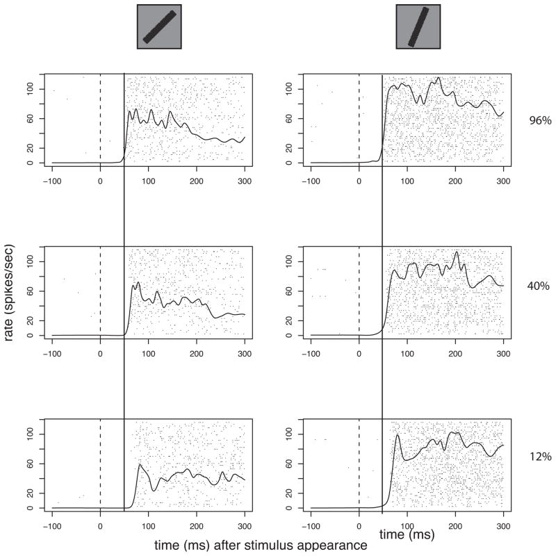
In early stages of visual processing in monkey, when a stimulus is stepped on within the receptive field of a neuron, the response begins after some delay (latency), thought to arise from the transmission from the retina to the site at which the neuronal recording takes place. So for example it is not unusual to see responses in the monkey lateral geniculate nucleus that begin 30–40 ms after the stimulus appears, and the earliest responses seen in primary visual cortex are on the order of 10 ms later. This timing can depend on the spatial configuration or other parameters, for example, the contrast, of the stimulus (Figure 1).
Figure 1.
Orientation and contrast affect two different parameters in supragranular V1 neuronal responses from rhesus monkey. The oriented bar at the top represents the stimulus flashed onto the receptive field of this neuron. The average number of spikes during the stimulus presentation changes with the orientation. As this example shows, the latency to response onset is closely related to the contrast. This example shows that the latency and average response strength can be independent, or nearly so. Thus, one important aspect of temporal coding, latency to response onset conveys, or at least emphasizes, different information than that conveyed by spike count. This example also demonstrates that counting spikes with respect to a fixed reference for all examples might induce a correlation with contrast that is really due to the delay in the response onset for lower contrast stimuli. For the rasters each line of dots shows the time of an action potential with reference to the stimulus appearance (vertical line at 0). The continuous line is a spike density plot formed by the convolution of a Gaussian pulse (σ = 3ms), converted to spikes/second/trial. The orientations of the two black bars are shown at the top of each column, and the luminance contrast is on the right of each row. This neuron shows the almost total absence of activity when there is no stimulus on the receptive field (to the left of time = 0).
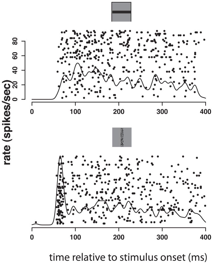
As the response evolves over time, there are response patterns that seem stereotyped, even if the number of spikes varies and the spikes are not seen at exactly the same time on repeated trials. For example, in V1 there may be a large transient burst of firing at the beginning of the stimulus-elicited firing, a feature that might be missing from the firing elicited by another pattern even when the number of spikes is the same (Figure 2).
Figure 2.
Equal strength responses from one supragranular V1 neuron with obvious differences in temporal encoding for 2 different stimuli, one a solid bar and the other a speckled bar orthogonal to the solid one, as shown above the responses.
A straightforward approach to analyzing both the number and pattern in the spike train is to take the principal components from the individual responses (Richmond and Optican, 1987). These provide the optimal linear basis set in the signal power or variance accounted for by each principal component; the principal components are ordered so that each principal component represents more variance than any of the preceding ones. This guarantees that any truncation will be the optimal linear representation. The coefficients of these principal components make a neural code. Because of the nature of the principal components, i.e., ordered by variance explained, it is likely that the earlier ones represent more information than the later ones, and this is generally the case.
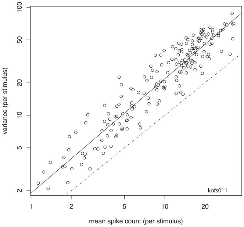
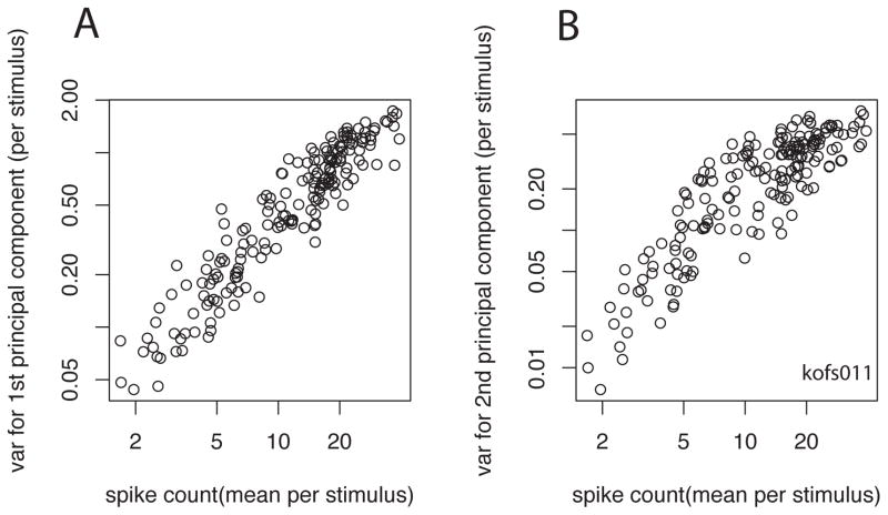
When stimuli are abruptly stepped on and then remain on for a few hundred milliseconds, both the number and timing of the spikes vary considerably across presentations of each stimulus, i.e., on different trials the number and timing of the spikes is different (cf. Figures 1 & 2). Nonetheless, the responses appear to be similar, and when low-pass filtered, i.e., convolved with Gaussian with standard deviation σ 3–5 ms; (Heller et al., 1995; Victor and Purpura, 1996). When the neuronal response variance across trials (either as the simple spike counts, or for the coefficients of the first or first 2–4 principal components) is calculated across a large number of stimuli and plotted as a function of the mean firing rates, the variance rises as a function of the firing rate, as is to be expected of a point process (Figure 3; (Dean, 1981; Tolhurst et al., 1983; Wiener and Richmond, 1999). The coefficients of the first principal component are usually closely related to the number of spikes in the response, indicating that the number of spikes is the strongest signal (i.e., accounting for the greatest variance) in the response (Figure 4; (Richmond and Optican, 1987; Richmond et al., 1990). Thus, it should be no surprise that the variance in the coefficients of the first principal component calculated on a stimulus-by-stimulus basis is directly related to the means of the first principal component (Figure 5A). Since the first principal component is strongly related to the spike count, the second principal component, which is by construction orthogonal to the first (the coefficients of the first and second are uncorrelated), must be related to some other feature of the responses, i.e., a pattern of spikes that accounts for a substantial proportion of variance. The variance of the second principal component is not very closely related to the mean of the second principal component (for the given stimulus set). Instead, the variance of the second principal component is also related to the means of the spike counts for the set of stimuli (Figure 5B). This shows that a great deal of the variation in the timing of the spikes is related to the variation in the spike count. If the patterns of spikes were just stochastically related to the spike count, i.e., when there are more spikes the number of spike patterns goes up, this is what we might expect to see. Imagine that the data arise from a Poisson process. Then the numbers of spike patterns observed will be related to the combinations of spikes that arise in such a Poisson process, which is , that is, n choose k or where the number of patterns that will arise from chance with n identical spikes distributed randomly into k bins. This consideration makes it seem entirely plausible that the variance in the second principal component, which is measuring a rate fluctuation that is (nearly) orthogonal to the mean rate, is related to the mean firing rate. This suggests that the number of patterns of spikes observed is arising from a process related to the number of spikes available, a seemingly obvious relationship. This again weighs in favor of the view that the spikes are stochastic samples of the underlying rate process.
Figure 3.
Variance of spike count as a function of spike count for 174 stimuli from one supragranular V1 neuron. On this log-log plot, the variance is linearly related (solid line) to the spike count. The relation here is ‘supra’ Poisson, that is, the regression line is offset above the line for which the variance equals the mean, which usually indicates some type of bursting. The stimulus set consisted of black bars, white bars, Walsh patterns, and speckled bars (cf Figure 2). All of the stimuli were presented, then the order was shuffled and they were presented again, for about 50 times (if the monkey broke fixation, which happened rarely, the response was not used here).
Figure 4.
A. Shapes of average response and first 5 principal components. The principal components are mutually orthogonal. All are plotted as probability of spiking as a function of time after stimulus appearance. The principal components are derived from low-pass filtered (3 ms σ Gaussian pulse) and sub-sampled (every 6 ms) spike densities of each trial. These principal components were calculated using all of the responses (~50 per stimulus) elicited by 174 stimuli (~8700 responses). As is standard, the average response was subtracted from each response before the data domain covariance matrix was calculated (thus translating the reference point to the mean of the data) which accounts for the negative values for some parts of some principal components, and for some of the coefficients in panel B. Each stimulus was stepped on for 360 ms. B. Average principal component coefficients for the first 5 principal components for the two stimuli shown in Figure 2. C. The reconstructed peristimulus spike densities (solid and dotted lines, matching those in Fig. 2) using the first 5 principal components (plus the mean). Because the mean response was subtracted from each response, each of the principal components weighted by the coefficient in panel B has been added to the average. High frequency components such as the low-level apparent oscillatory activity in the originals in Figure 2 are reduced or eliminated because the higher principal components have been left out. Thus, this reconstruction with only 5 principal components has the effect of additional low-pass filtering (after the Gaussian convolution described above) the responses.
Figure 5.
Mean variance relations between spike counts for each of the 174 stimuli (x-axis) and variance of 1st (left panel) or 2nd principal components for the corresponding stimulus. This shows that the variance of the coefficients of the 2nd principal component is linearly related to the mean spike counts, just as is true for the spike count variance and 1st principal component variance.
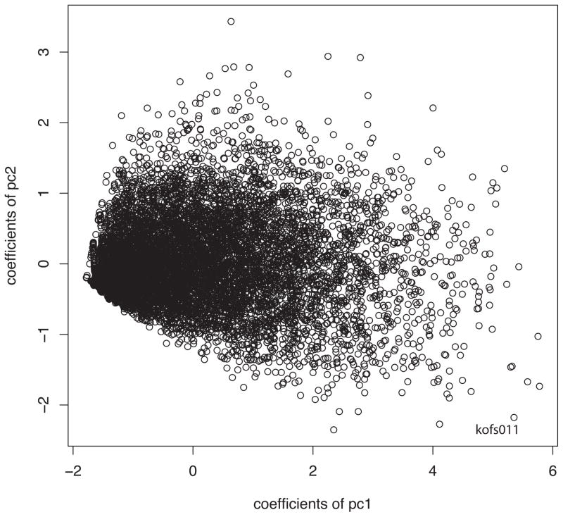
There is one additional observation related to the principal components that raises the possibility that the spikes arise from a stochastic process. When the coefficients of the second principal components are plotted as functions of the coefficients of the first principal component, the data fit into a cone (Figure 6). This shows that the number of spike patterns, a parameter that is better related to the second principal component, increases as the spike count increases, although the number of patterns grows somewhat more slowly (not shown; see (Wiener and Richmond, 2003) than would be expected from a purely Poisson process (one limitation is the refractory period).
Figure 6.
Coefficients of second principal component vs coefficients of first principal component for each stimulus presentation. The narrow distribution at the left is a consequence of the spike trains being point processes. Because the first principal component is nearly the spike count, the number of spikes available for patterns of activity increases from left to right, so the number of patterns possible is small for low spike counts (left side of plot). Then numbers of spike patterns represented by the second principal component increase quickly with the increasing spike count, making for the cone-like structure in this plot. This shows that even though the principal components are orthogonal, they are not independent; higher coefficients of the first principal component lead to a larger range of values for the second.
Stochastic spike trains
The findings above support a hypothesis that the spike train is a stochastic sampling of some underlying perhaps continuous distribution. Given the evidence, it is reasonable to develop and investigate a description of spike trains in which spikes are stochastic samples of underlying distributions, even if the trains are not Poisson, i.e., stochastic does not necessarily mean Poisson.
Now let us generalize. We will no longer require either a constant firing rate, or even a time-varying Poisson process. We will still require that the spikes arise from a stochastic renewal process. What happens when the spikes are stochastic, but not necessarily Poisson, samples from a continuous, deterministic processes, i.e., from the rate function or spike density over time (for example, continuous lines in Figure 1)? The intuition for our model is that the spike train for the trials can be simulated as a simple rate-varying Poisson process, and the distribution of spike counts is controlled so that they match the observed distribution of spike counts. To obtain simulated spike trains that on average match our recorded data, we use the normalized spike probability density over time, or peristimulus time histogram, to get a rate variation function over time. Because we have shown that the deviations from a Poisson process can be matched by matching the spike count distributions from our recorded data (Oram et al., 1999), we then simulate spike trains and pick those that meet our requirements for the number of spikes. We can even easily incorporate the absolute refractory period by only picking simulated trials that have no intervals as short as 1 millisecond (1 bin in our simulations). Under these conditions the numbers of spike patterns we observe are statistically indistinguishable from those observed in the spike trains (Oram et al., 1999).
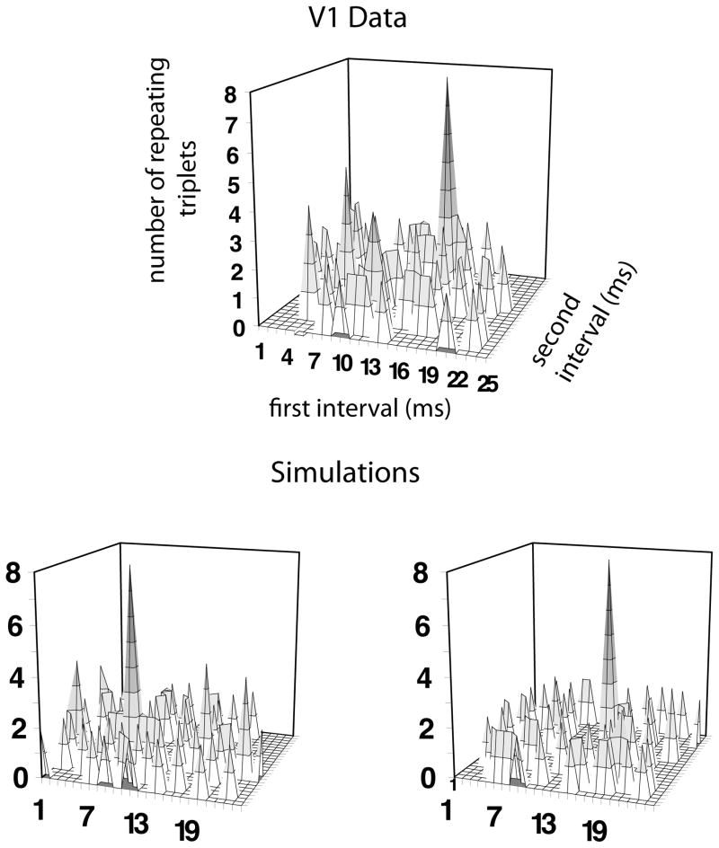
When the data from these simulated spike trains are analyzed, the numbers of triplets over the set of two intervals (that is, the number of triplets for each pair of intervals is counted forming joint-interval histograms) are indistinguishable from the ones seen in the real data. Thus, when the spike count distributions of the data and simulation match, the distributions of spike timings, i.e., the joint interval histograms, that are seen in the physiological data are compatible with this constrained stochastic process. Furthermore, the numbers of patterns can have high individual peaks for particular patterns (Figure 7). When the simulations are run again, the highest peaks are related to different patterns than in the original simulations. On examination of the simulated data, the numbers of preferred patterns seen in the data are within the numbers that might be expected from a stochastic process (derived from the simulations), suggesting that the preferred patterns seen in the physiological data could arise as a consequence of a stochastic process.
Figure 7.
Numbers of triplets arising in the data of one V1 supragranular neuron (upper panel), and the numbers of triplets arising in two simulation runs of 104 each using the simple spike count matching model with refractory period (see text). When the numbers of triplets in the data are correlated with the numbers of triplets in the simulations over the stimuli, the linear correlation is r > 0.99.
This simple model does not provide a means to interpret what mechanisms contribute to the deviation from a true Poisson process, but it does show that for data like those we have sampled in the visual and motor systems, matching the spike count distribution to that seen from the recordings is a strong enough constraint to create a stochastic model of the spike trains that is indistinguishable from the data.
Order statistics for modeling and analyzing spike trains
These considerations lead to a model in which the pattern of the spikes over time arise as if they were thrown down with probabilities given by the rate function, that is, they are stochastic samples from a deterministic rate function. This simple model is described by order statistics. Order statistics describes how a stochastic point process with n ordered points sample an underlying distribution, here the normalized spike density over time (Arnold et al., 1992). Specifically, the fundamental equation in order statistics describes the unconditional distribution in time of when the kth of n spikes will occur when t=0 is the beginning of an interval of interest, e.g., when a stimulus appears and disappears:
where F(t) is the cumulative probability distribution for the rate variation function (the integrated spike density or PSTH), f(t) is the normalized perstimulus time spike density (histogram), and hn,s(t) is the order statistic for the probability of a spike at time t in a train of n spikes for stimulus s. This completely describes stochastic spike trains, and, therefore, provides a strong null hypothesis for testing whether spike trains are stochastic, overcoming a potentially dangerous limitation of having to assume a Poisson process in particular. This order statistic approach provides a straightforward, well-developed description that can be used to make both a generative model for spike trains, and an interpretive (decoding) model (see below).
The probability distribution for the first spike out of n spikes starting at some time, t=0, such as the stimulus appearance, is:
Now summing over n, the probability of the first spike across the distribution of spike counts (estimated from the data, or chosen from an a priori hypothesis) for the stimulus is:
where ps(n)is the probability of n spikes given the stimulus s. Furthermore, we recognize that 1 − hs (t) is the probability of stimulus s at time t when there is no spike. This provides the machinery needed to decode spike trains, millisecond-by-millisecond, or to estimate the mutual information. Now it is completely straightforward to apply Bayes theorem to decode millisecond-by-millisecond:
So we have an expression that calculates the probability of each stimulus, given a spike at time t, or when there is no spike. That is, p(s|t) can all be calculated for each stimulus at each time step when there is no spike, or when there is a spike. When a spike does occur, the first order statistics are recalculated using the time t as the new reference time, that is, a new t=0. The set of p(s\t) at that point is used for the new prior probabilities, p(s), for all of the stimuli (Figure 8). Using this recursive relation, we can decode the stimulus as the response unfolds.
Figure 8.
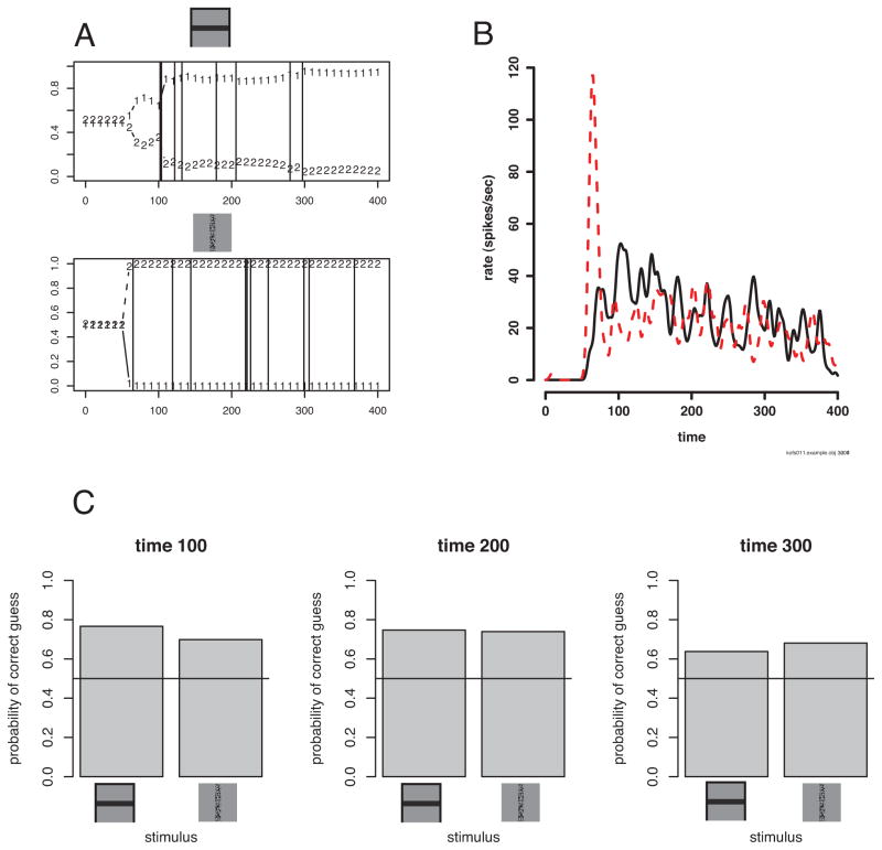
Decoding of example from Figure 2. A. Millisecond-by-millisecond decoding for two spike trains with spike times shown as vertical lines. Because there are two stimuli in this example, the probability for random guessing is 0.5. B. The overlaid spike densities from Figure 2. The dashed line is the spike density for the speckled vertical bar and the solid line is for the horizontal black bar. This helps to explain the decoding, which starts before a spike for the black bar, because the decoder knows that if no spike has occurred by this time, the black bar is more likely. The value of the decoder is that it points to this feature of the spike densities. C. The decoding performance over the approximately 50 trials with each stimulus. The decoding accuracy does not improve after 100 ms for this example.
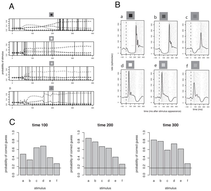
The algebra above depends on the assumption that the spike trains are stochastic samples using the spike count distributions and the rate functions estimated from the data. This approach seems to work well. Here are two brief examples, one taken from a V1 supragranular (layers 2 or 3) complex cell, where the baseline firing rate is just about zero (Figure 8), and the other from LGN recordings where neurons have baseline (un-stimulated) firing rates of about 40 Hz (Figure 9). This decoding strategy works well in both circumstances.
Figure 9.
Decoding examples for neurons that have ongoing activity as is often seen in monkey LGN neurons. A. Decodings for 4 example responses (chosen to end correctly). The stimuli are shown above. The vertical lines show the spike times. The lower-case letters a–g show the probability that the response seen until the time examined was elicited by each stimulus seen in panel B. The horizontal line shows the 1/6 prior probability assuming random guessing. B. The rasters and spike density for the 6 different stimuli shown in this example. These were all square spots positioned on the receptive field and flashed on for 250 ms each. Notice the off-responses. C. The decoding performance for each of the stimuli at 3 different times during the stimulus cycle. The decoding performance is different across the stimuli, and leads to the conclusion that some stimuli are more easily mistaken (misidentified) for others. Also, decoding improves with time, with the best average decoding occurring at 300 ms after stimulus appearance.
What has been shown above is that a model in which spike trains are treated as stochastic samples provides a powerful tool for analyzing firing. A substantial number of experiments have been carried out that seem to show remarkable reproducibility of spikes across stimulations(Bryant and Segundo, 1976; Mainen and Sejnowski, 1995; Bair and Koch, 1996; Buracas et al., 1998; Butts et al., 2007). The question is whether the order statistic approach would work well in these situations. It would likely still work because the response features are time-locked to the stimulus or other trial event. In many, if not all, of these experiments, one can make the observation that the stimulus had some strong time-changing characteristic, that is, there was strong motion or luminance steps(Williams et al., 2004). Also, whereas the data from many of these experiments have been subjected to rigorous analysis, none of them have been tested against an order-statistic based hypothesis. What would be expected under such conditions? For the hypothesis, the spike density and spike count distributions would need to be measured. Then simulations would be made using these to determine whether the spike trains in the recorded data fell outside of the confidence intervals for the simulated data, where the confidence intervals are estimated from the variability arising from a large number of simulation runs, e.g., 103 or 104.
Unsettled issues and conclusions
An unsettled issue is whether there are hidden patterns that are not time-locked to events in the recordings, perhaps giving a clue to whether there are undetected processes underlying the generation of spike trains. The strongest early hypotheses about the existence of such patterns arose from the work of Abeles, and Lestienne and Stehler (Lestienne and Strehler, 1987; Abeles and Gerstein, 1988; Abeles et al., 1993). This remains a fascinating area of work, that in a manner of speaking harkens back to the original calculation done by Mackay and McCullough, in that they had to suppose that all patterns were available for use in coding (MacKay and McCullough, 1952). The order statistic hypothesis shows that processes deviating from a Poisson process make significant differences in the numbers of patterns that are predicted to arise in spike trains from stochastic processes (triplets above). The hidden pattern hypothesis is based on the idea that the dynamics of the system favor the occurrence of specific spike patterns arising when system architecture is appropriate,.e.g., synfire chains (Lestienne and Strehler, 1987; Abeles and Gerstein, 1988; Abeles, 1991).
At this point, it is clear, as it has been for more than 75 years, that the strongest part of the neural code is the spiking rate (Adrian and Bronk, 1928, 1929), with the single most critical parameter generally being the mean rate. However, there is also strong evidence that temporal encoding, at least in the form of rate variation, is also an important feature of the code. What is established above is that the spike counts over moderate counting periods show considerable variability. The pattern of the spikes over time is taken to arise as a stochastic sample of a deterministic rate function. These two properties lead to a model in which spikes arise as if they were thrown down with probabilities given by the rate function.
Because of the interaction between the number of spikes and sampling of underlying continuous processes, patterns of spiking activity need to be interpreted with care, and many details probably do matter in coming to conclusions about whether activity is stochastic or not. Although not discussed here, the properties described above have important influences on the relations between neurons, i.e., the peaks in cross-correlograms can arise from purely stochastic considerations (Brody, 1998; Oram et al., 2001). Strong sensory signals can be reflected in a temporal code that follows the driving rate, and while it has not been tested, it would not be surprising to find that these also have the properties described above.
What is clear is that assuming that spikes arise as a stochastic, but not necessarily, Poisson point process is a powerful null hypothesis, and because of the vast modern attention to the properties of point processes using order statistics, the description provides a strong null hypothesis that can be used in both generative and analysis (decoding and mutual information) models. This approach does not require utilizing the exact timing of every spike, but rather substitutes a connection between relatively simple measurements of neuronal responses, the peristimulus time histogram, and estimates of its bandwidth (not discussed above except implicitly with reference to rapid motion energy stimuli), the distribution of observed spike counts, and the structure of spike trains. Because we are interested in functionality, not just signal strength, the possibility must remain that some network properties of importance could be signaled through the existence of seemingly nonstochastic patterns, such as triplets (Abeles, 1991). At this time, deviations from this order statistic model seem to be small, and therefore, if considered in signal-to-noise terms, account for very little signal strength. Thus, the experimental evidence reviewed above suggests patterns of spikes are indistinguishable from what would be expected from a stochastic point process, and modeling the trains from that point of view is a powerful approach to describing them.
Acknowledgments
This work was supported by the Intramural Program of NIH/NIMH.
References
- Abeles M. Corticonics. Cambridge, UK: Cambridge Univ. Press; 1991. [Google Scholar]
- Abeles M, Gerstein GL. Detecting spatiotemporal firing patterns among simultaneously recorded single neurons. J Neurophysiol. 1988;60:909–924. doi: 10.1152/jn.1988.60.3.909. [DOI] [PubMed] [Google Scholar]
- Abeles M, Bergman H, Margalit E, Vaadia E. Spatiotemporal firing patterns in the frontal cortex of behaving monkeys. J Neurophysiol. 1993;70:1629–1638. doi: 10.1152/jn.1993.70.4.1629. [DOI] [PubMed] [Google Scholar]
- Adrian ED, Bronk DW. The discharge of impulses in motor nerve fibres: Part I. Impulses in single fibres of the phrenic nerve. J Physiol. 1928;66:81–101. doi: 10.1113/jphysiol.1928.sp002509. [DOI] [PMC free article] [PubMed] [Google Scholar]
- Adrian ED, Bronk DW. The discharge of impulses in motor nerve fibres: Part II. The frequency of discharge in reflex and voluntary contractions. J Physiol. 1929;67:i3–151. [PMC free article] [PubMed] [Google Scholar]
- Arnold BC, Balakrishnan N, Nagarajan HN. A first course in order statistics. New York: Wiley; 1992. [Google Scholar]
- Bair W, Koch C. Temporal precision of spike trains in extrastriate cortex of the behaving macaque monkey. Neural Comput. 1996;8:1185–1202. doi: 10.1162/neco.1996.8.6.1185. [DOI] [PubMed] [Google Scholar]
- Brody CD. Slow covariations in neuronal resting potentials can lead to artefactually fast cross-correlations in their spike trains. J Neurophysiol. 1998;80:3345–3351. doi: 10.1152/jn.1998.80.6.3345. [DOI] [PubMed] [Google Scholar]
- Bryant HL, Segundo JP. Spike initiation by transmembrane current: a white-noise analysis. J Physiol. 1976;260:279–314. doi: 10.1113/jphysiol.1976.sp011516. [DOI] [PMC free article] [PubMed] [Google Scholar]
- Buracas GT, Zador AM, DeWeese MR, Albright TD. Efficient discrimination of temporal patterns by motion-sensitive neurons in primate visual cortex. Neuron. 1998;20:959–969. doi: 10.1016/s0896-6273(00)80477-8. [DOI] [PubMed] [Google Scholar]
- Butts DA, Weng C, Jin J, Yeh CI, Lesica NA, Alonso JM, Stanley GB. Temporal precision in the neural code and the timescales of natural vision. Nature. 2007;449:92–95. doi: 10.1038/nature06105. [DOI] [PubMed] [Google Scholar]
- Dean AF. The variability of discharge of simple cells in the cat striate cortex. Exp Brain Res. 1981;44:437–440. doi: 10.1007/BF00238837. [DOI] [PubMed] [Google Scholar]
- Fitzhugh R. The statistical detection of threshold signals in the retina. J Gen Physiol. 1957;40:925–948. doi: 10.1085/jgp.40.6.925. [DOI] [PMC free article] [PubMed] [Google Scholar]
- Gawne TJ, Richmond BJ. How independent are the messages carried by adjacent inferior temporal cortical neurons? J Neurosci. 1993;13:2758–2771. doi: 10.1523/JNEUROSCI.13-07-02758.1993. [DOI] [PMC free article] [PubMed] [Google Scholar]
- Gawne TJ, Kjaer TW, Hertz JA, Richmond BJ. Adjacent visual cortical complex cells share about 20% of their stimulus-related information. Cereb Cortex. 1996;6:482–489. doi: 10.1093/cercor/6.3.482. [DOI] [PubMed] [Google Scholar]
- Georgopoulos AP, Kettner RE, Schwartz AB. Primate motor cortex and free arm movements to visual targets in three-dimensional space. II. Coding of the direction of movement by a neuronal population. J Neurosci. 1988;8:2928–2937. doi: 10.1523/JNEUROSCI.08-08-02928.1988. [DOI] [PMC free article] [PubMed] [Google Scholar]
- Heller J, Hertz JA, Kjaer TW, Richmond BJ. Information flow and temporal coding in primate pattern vision. J Comput Neurosci. 1995;2:175–193. doi: 10.1007/BF00961433. [DOI] [PubMed] [Google Scholar]
- Kuffler SW, Fitzhugh R, Barlow HB. Maintained activity in the cat’s retina in light and darkness. J Gen Physiol. 1957;40:683–702. doi: 10.1085/jgp.40.5.683. [DOI] [PMC free article] [PubMed] [Google Scholar]
- Lestienne R, Strehler BL. Time structure and stimulus dependence of precisely replicating patterns present in monkey cortical neuronal spike trains. Brain Res. 1987;437:214–238. doi: 10.1016/0006-8993(87)91638-6. [DOI] [PubMed] [Google Scholar]
- MacKay DM. Neural communications: experiment and theory. Science. 1968;159:335–353. doi: 10.1126/science.159.3812.335. [DOI] [PubMed] [Google Scholar]
- MacKay DS, McCullough WS. The limiting information capacity of a neuronal link. Bull Math Math Biophysics. 1952;14:127–135. [Google Scholar]
- Mainen ZF, Sejnowski TJ. Reliability of spike timing in neocortical neurons. Science. 1995;268:1503–1506. doi: 10.1126/science.7770778. [DOI] [PubMed] [Google Scholar]
- Moore GP, Perkel DH, Segundo JP. Statistical analysis and functional interpretation of neuronal spike data. Annu Rev Physiol. 1966;28:493–522. doi: 10.1146/annurev.ph.28.030166.002425. [DOI] [PubMed] [Google Scholar]
- Oram MW, Wiener MC, Lestienne R, Richmond BJ. Stochastic nature of precisely timed spike patterns in visual system neuronal responses. J Neurophysiol. 1999;81:3021–3033. doi: 10.1152/jn.1999.81.6.3021. [DOI] [PubMed] [Google Scholar]
- Oram MW, Hatsopoulos NG, Richmond BJ, Donoghue JP. Excess synchrony in motor cortical neurons provides redundant direction information with that from coarse temporal measures. J Neurophysiol. 2001;86:1700–1716. doi: 10.1152/jn.2001.86.4.1700. [DOI] [PubMed] [Google Scholar]
- Richmond BJ, Optican LM. Temporal encoding of two-dimensional patterns by single units in primate inferior temporal cortex. II. Quantification of response waveform. J Neurophysiol. 1987;57:147–161. doi: 10.1152/jn.1987.57.1.147. [DOI] [PubMed] [Google Scholar]
- Richmond BJ, Optican LM, Spitzer H. Temporal encoding of two-dimensional patterns by single units in primate primary visual cortex. I. Stimulus-response relations. J Neurophysiol. 1990;64:351–369. doi: 10.1152/jn.1990.64.2.351. [DOI] [PubMed] [Google Scholar]
- Salinas E, Abbott LF. Vector reconstruction from firing rates. J Comput Neurosci. 1994;1:89–107. doi: 10.1007/BF00962720. [DOI] [PubMed] [Google Scholar]
- Segundo JP, Moore GP, Stensaas LJ, Bullock TH. Sensitivity of Neurones in Aplysia to Temporal Pattern of Arriving Impulses. J Exp Biol. 1963;40:643–667. doi: 10.1242/jeb.40.4.643. [DOI] [PubMed] [Google Scholar]
- Shadlen MN, Britten KH, Newsome WT, Movshon JA. A computational analysis of the relationship between neuronal and behavioral responses to visual motion. J Neurosci. 1996;16:1486–1510. doi: 10.1523/JNEUROSCI.16-04-01486.1996. [DOI] [PMC free article] [PubMed] [Google Scholar]
- Sugase Y, Yamane S, Ueno S, Kawano K. Global and fine information coded by single neurons in the temporal visual cortex. Nature. 1999;400:869–873. doi: 10.1038/23703. [DOI] [PubMed] [Google Scholar]
- Tolhurst DJ, Movshon JA, Dean AF. The statistical reliability of signals in single neurons in cat and monkey visual cortex. Vision Res. 1983;23:775–785. doi: 10.1016/0042-6989(83)90200-6. [DOI] [PubMed] [Google Scholar]
- Victor JD, Purpura KP. Nature and precision of temporal coding in visual cortex: a metric-space analysis. J Neurophysiol. 1996;76:1310–1326. doi: 10.1152/jn.1996.76.2.1310. [DOI] [PubMed] [Google Scholar]
- Wiener MC, Richmond BJ. Using response models to estimate channel capacity for neuronal classification of stationary visual stimuli using temporal coding. J Neurophysiol. 1999;82:2861–2875. doi: 10.1152/jn.1999.82.6.2861. [DOI] [PubMed] [Google Scholar]
- Wiener MC, Richmond BJ. Decoding spike trains instant by instant using order statistics and the mixture-of-Poissons model. J Neurosci. 2003;23:2394–2406. doi: 10.1523/JNEUROSCI.23-06-02394.2003. [DOI] [PMC free article] [PubMed] [Google Scholar]
- Wiersma CAG, Adams RT. The influence of nerve impulse sequence on the contractions of different crustacean muscles. Physiol comp et oeco. 1950;2:20–33. [Google Scholar]
- Williams PE, Mechler F, Gordon J, Shapley R, Hawken MJ. Entrainment to video displays in primary visual cortex of macaque and humans. J Neurosci. 2004;24:8278–8288. doi: 10.1523/JNEUROSCI.2716-04.2004. [DOI] [PMC free article] [PubMed] [Google Scholar]


