Additive Genetic Variability and the Bayesian Alphabet

Abstract

The use of all available molecular markers in statistical models for prediction of quantitative traits has led to what could be termed a genomic-assisted selection paradigm in animal and plant breeding. This article provides a critical review of some theoretical and statistical concepts in the context of genomic-assisted genetic evaluation of animals and crops. First, relationships between the (Bayesian) variance of marker effects in some regression models and additive genetic variance are examined under standard assumptions. Second, the connection between marker genotypes and resemblance between relatives is explored, and linkages between a marker-based model and the infinitesimal model are reviewed. Third, issues associated with the use of Bayesian models for marker-assisted selection, with a focus on the role of the priors, are examined from a theoretical angle. The sensitivity of a Bayesian specification that has been proposed (called “Bayes A”) with respect to priors is illustrated with a simulation. Methods that can solve potential shortcomings of some of these Bayesian regression procedures are discussed briefly.

IN an influential article on animal breeding, Meuwissen et al. (2001) suggested using all available molecular markers as covariates in linear regression models for prediction of genetic value for quantitative traits. This has led to a genome-enabled selection paradigm. For example, major dairy cattle breeding countries are now genotyping elite animals and genetic evaluations based on SNPs (single nucleotide polymorphisms) are becoming routine (Hayes et al. 2009; van Raden et al. 2009). A similar trend is taking place in poultry (e.g., Long et al. 2007; González-Recio et al. 2008, 2009), beef cattle (D. J. Garrick, personal communication), and plants (Heffner et al. 2009).

The extraordinary speed with which events are taking place hampers the process of relating new developments to extant theory, as well as the understanding of some of the statistical methods proposed so far. These span from Bayes hierarchical models (e.g., Meuwissen et al. 2001) and the Bayesian Lasso (e.g., de los Campos et al. 2009b) to ad hoc procedures (e.g., van Raden 2008). Another issue is how parameters of models for dense markers relate to those of classical models of quantitative genetics.

Many statistical models and approaches have been proposed for marker-assisted selection. These include multiple regression on marker genotypes (Lande and Thompson 1990), best linear unbiased prediction (BLUP) including effects of a single-marker locus (Fernando and Grossman 1989), ridge regression (Whittaker et al. 2000), Bayesian procedures (Meuwissen et al. 2001; Gianola et al. 2003; Xu 2003; de los Campos et al. 2009b), and semiparametric specifications (Gianola et al. 2006a; Gianola and de los Campos 2008). In particular, the methods proposed by Meuwissen et al. (2001) have captured enormous attention in animal breeding, because of several reasons. First, the procedures cope well with data structures in which the number of markers amply exceeds the number of observations, the so-called “small n, large p” situation. Second, the methods in Meuwissen et al. (2001) constitute a logical progression from the standard BLUP widely used in animal breeding to richer specifications, where marker-specific variances are allowed to vary at random over many loci. Third, Bayesian methods have a natural way of taking into account uncertainty about all unknowns in a model (e.g., Gianola and Fernando 1986) and, when coupled with the power and flexibility of Markov chain Monte Carlo, can be applied to almost any parametric statistical model. In Meuwissen et al. (2001) normality assumptions are used together with conjugate prior distributions for variance parameters; this leads to computational representations that are well known and have been widely used in animal breeding (e.g., Wang et al. 1993, 1994). An important question is that of the impact of the prior assumptions made in these Bayesian models on estimates of marker effects and, more importantly, on prediction of future outcomes, which is central in animal and plant breeding.

A second aspect mentioned above is how parameters from these marker-based models relate to those of standard quantitative genetics theory, with either a finite or an infinite number (the infinitesimal model) of loci assumed. The relationships depend on the hypotheses made at the genetic level and some of the formulas presented, e.g., in Meuwissen et al. (2001), use linkage equilibrium; however, the reality is that marker-assisted selection relies on the existence of linkage disequilibrium. While a general treatment of linkage disequilibrium is very difficult in the context of models for predicting complex phenotypic traits, it is important to be aware of its potential impact. Another question is the definition of additive genetic variance, according to whether marker effects are assumed fixed or random, with the latter corresponding to the situation in which such effects are viewed as sampled randomly from some hypothetical distribution. Meuwissen et al. (2001) employ formulas for eliciting the variance of marker effects, given some knowledge of the additive genetic variance in the population. Their developments begin with the assumption that marker effects are fixed, but these eventually become random without a clear elaboration of why this is so. Since their formulas are used in practice for eliciting priors in the Bayesian treatment (e.g., Hayes et al. 2009), it is essential to understand their ontogeny, especially considering that priors may have an impact on prediction of outcomes.

The objective of this article is to provide a critical review of some of these aspects in the context of genomic-assisted evaluation of quantitative traits. First, relationships between the (Bayesian) variance of marker effects in some regression models and additive genetic variance are examined. Second, connections between marker genotypes and resemblance between relatives are explored. Third, the liaisons between a marker-based model and the infinitesimal model are reviewed. Fourth, and in the context of the quantitative genetics theory discussed in the preceding sections, some statistical issues associated with the use of Bayesian models for (massive) marker-assisted selection are examined, with the main focus on the role of the priors. The sensitivity of some of these methods with respect to priors is illustrated with a simulation.

RELATIONSHIP BETWEEN THE VARIANCE OF MARKER EFFECTS AND ADDITIVE GENETIC VARIANCE

Additive genetic variance:

A simple specification serves to set the stage. The phenotypic value (y) for a quantitative trait is described by the linear model

(1)

where a is the additive effect of a biallelic locus on the trait, w is a random indicator variable (covariate) relating a to the phenotype, and E is an independently distributed random deviate, , where V_E is the environmental or residual variance, provided gene action is additive. Under Hardy–Weinberg (HW) equilibrium, the frequencies of the three possible genotypes are , and , where and . Code arbitrarily the states of w such that

(2)

The genetic values of MM, Mm, and mm individuals are a, 0, and −a, respectively. Then

(3)

(4)

and

(5)

This is the variance among genotypes (not among their genetic values) at the locus under HW equilibrium.

A standard treatment (e.g., Falconer and Mackay 1996) regards the additive effect a as a fixed parameter. The conditional distribution of phenotypes, given a (but unconditionally with respect to w, since genotypes vary at random according to HW frequencies), has mean

(6)

and variance

(7)

where V_A = 2pqa² is the additive genetic variance at the locus. In this standard treatment, the additive genetic variance depends on the additive effect a but not on its variance; unless a is assigned a probability distribution, it does not possess variance.

Uncertainty about the additive effect:

Assume now that , where θ is the mean of the distribution. In the Appendix of Meuwissen et al. (2001), a suddenly mutates from fixed to random without explanation. How does the variance of a arise? Parameter can be assigned at least two interpretations. The first one is as the variance between a effects in a conceptual sampling scheme in which such effects are drawn at random from a population of loci. In the second (Bayesian), represents uncertainty about the true but unknown value of the additive effect of the specific locus, but without invoking a scheme of random sampling over a population of loci. For example, = 0 means in a Bayesian sense that a = θ with complete certainty, but not necessarily that the locus does not have an effect, since θ may (may not) be distinct from 0; this cannot be overemphasized. With a single locus the Bayesian interpretation is more intuitive, since it is hard to envisage a reference population of loci in this case.

Irrespective of the interpretation assigned to , the assumption induces another conditional distribution (given w) with mean and variance

(8)

and

(9)

respectively. However, both w (the genotypes) and a (their effects) are now random variables possessing a joint distribution. Here, it is assumed that w and a are independent, but this may not be so, as in a mutation-stabilizing selection model (e.g., Turelli 1985) or in situations discussed by Zhang and Hill (2005) where the distribution of gene frequencies after selection depends on a. Deconditioning over both a and w (that is, averaging over all genotypes at the locus and all values that a can take), the expected value and variance of the marginal distribution of y are

(10)

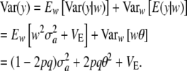
and

(11)

This distribution is not normal: the phenotype results from multiplying a discrete random variable w by the normal variate a, and then adding a deviate E, which may or may not be normal, depending on what is assumed about the residual distribution. The genetic variance is now . The term stems from randomness (uncertainty) about a, and it dissipates from (11) only if = 0. Note that there is additive genetic variance even if = 0, and it is equal to 2pqθ². Further, if the standard assumption θ = 0 is adopted, the variance of the marginal distribution of phenotypes becomes

(12)

Here, the standard term for additive genetic variance disappears and yet may not be zero, since one poses that a locus has no effect (on average) but there is some uncertainty or variation among loci effects, as represented by .

In a nutshell, the additive genetic variance at the locus, V_A = 2pqa², does not appear in (11), because a has been integrated out; actually, it is replaced by 2pqθ² in (11). The term does not arise in the standard (fixed) model, where additive genetic variance in stricto sensu is V_A. When a is known with certainty, then = 0 and yet the locus generates additive genetic variance, as measured by V_A = 2pqθ². If θ = 0 and = 0, then the variance is purely environmental. In short, the connection between the uncertainty variance and the additive variance V_A (which involves the effect of the locus) is elusive when both genotypes and effects are random variables.

Several loci:

Consider now K loci with additive effect a_k at locus k, without dominance or epistasis. The phenotype is expressible as

(13)

with under HW equilibrium. If all markers were quantitative trait loci (QTL), this would be a “finite number of QTL” model; it is assumed that these loci are markers hereinafter unless stated otherwise. Under this specification

(14)

To deduce the additive variance, some assumption must be made about the joint distribution of w₁, w₂,…, w_K, the genotypes at the K loci.

Linkage equilibrium (LE) and HW frequencies are assumed to make the problem tractable. Some expressions are available to accommodate linkage disequilibrium, but parameters are not generally available to evaluate them (see the appendix). When there is selection, genetic drift, or introgression and many loci are considered jointly, some of which will be even physically linked, the LE assumption is unrealistic. Hence, as in the case of many other authors, e.g., Barton and de Vladar (2009) in a study of evolution of traits using statistical mechanics, LE–HW assumptions are used here.

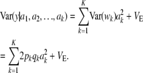
If there is LE, the distributions of genotypes at the K loci are mutually independent, so that

(15)

The multilocus additive genetic variance under LE–HW is then .

Suppose now that all effects a_k are drawn from the same random process with some distribution function , mean θ, and variance . Using the same reasoning as before, the variance of the marginal distribution of the phenotypes is

(16)

Then

(17)

which generalizes (11) to K loci. The first term is variance due to uncertainty, the second term is the standard additive genetic variance, and the third one is residual variation.

What is the relationship between the multilocus additive genetic variance and ? Let be the mean variance, obtained by averaging V_A over the distribution of the a's. This operation yields

Hence, if θ = 0 (additive effects expressed as a deviation from their mean), then

(18)

The relationship between the uncertainty variance and the marked average additive genetic variance would then be

(19)

in agreement with Habier et al. (2007), but different from Meuwissen et al. (2001). Unless the markers are QTL, gives only the part of the additive genetic variance captured by markers, and this may be a tiny fraction only (Maher 2008). This makes the connection between additive genetic variance for a trait and marked variance even more elusive.

Corresponding formulas under linkage disequilibrium are in the appendix.

Heterogeneity of variance:

Suppose now that locus effects are independently (but not identically) distributed as . The mean of the marginal distribution of phenotypes is , and the variance becomes

If all = 0 (complete Bayesian certainty about all marker effects a_k), there would still be genetic variance, as measured by the second term in . Apart from the difficulty of inferring a given with any reasonable precision, there is the question of possible “commonality” between locus effects. For instance, some loci may have correlated effects, and alternative forms for the prior distribution of the a's have been suggested by Gianola et al. (2003). Also, some of these effects are expected to be identically equal to 0, especially if a_k represents a marker effect, as opposed to being the result of a QTL [if the marker is in linkage disequilibrium (LD) with the QTL, its effect would be expected to be nonnull]. In such a case, a more flexible prior distribution might be useful, such as a mixture of normals, a double exponential, or a Dirichlet process.

If a frequentist interpretation is adopted for the assumption , it is difficult to envisage the conceptual population from which a_k is sampled, unless the variances are also random draws from some population. Posing a locus-specific variance is equivalent to assuming that each sire in a sample of Holsteins is drawn from a different conceptual population with sire-specific variance. There would be as many variances as there are sires!

Variation in allelic frequencies:

In addition to assuming random variation of a effects over loci, a distribution of gene frequencies may be posed as well. Wright (1937) found that a beta distribution arose from a diffusion equation that was used to study changes in allele frequencies in finite populations, so this is well grounded in population genetics. In a Bayesian context, on the other hand, assigning a beta distribution to gene frequencies would be a (mathematically convenient) representation of uncertainty.

Suppose that allelic frequencies p_k (k = 1, 2,…, K) vary over loci according to the same beta process, where φ_a, φ_b are parameters determining the form of the distribution; Wright (1937) expressed these parameters as functions of effective population size and mutation rates. Standard results yield

(20)

(21)

and

(22)

The expected heterozygosity is given by

(23)

There are now four sources of variation: (1) due to random sampling of genotypes over individuals in the population, (2) due to uncertainty about additive effects (equivalently, variability due to sampling additive effects over loci), (3) due to spread of gene frequencies over loci or about some equilibrium distribution, and (4) environmental variability. The third source contributes to variance under conceptual repeated sampling, since gene frequencies would fluctuate around the equilibrium distribution or over loci.

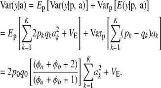
Consider now additive genetic variance when dispersion in allelic frequencies is taken into account, assuming LE. Let and . Using previous results, (22) and (23),

(24)

The expected additive genetic variance is now

(25)

To arrive at the marginal distribution of phenotypes, variation in a effects is brought into the picture, producing the variance decomposition

(26)

after variation in genotypes and frequencies (i.e., with respect to w and p) has been taken into account. From (13)

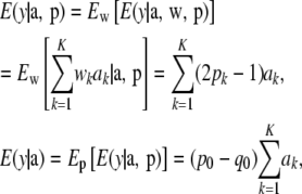so that in the absence of correlations between locus effects

(27)

Likewise, using (24),

(28)

Combining (27) and (28) as required by (26) leads to

(29)

The variance of the marginal distribution of the phenotypes has, thus, three components. The one involving relates to uncertainty about or random variation of marker effects. The second,

is exactly the additive genetic variance when the mean of the distribution of marker effects is known with complete certainty, and the third component is the environmental variance V_E. If θ = 0 and the first term of (29) is interpreted as additive genetic variance (), it turns out that

(30)

This is similar to Habier et al. (2007) only if p₀ = q₀, φ_a + φ_b is large enough, and K is very large, such that

where is the beta density representing variation of allelic frequencies.

RESEMBLANCE BETWEEN RELATIVES

Standard results:

QTL are most often unknown, so their effects and their relationships to those of markers are difficult to model explicitly. An alternative is to focus on effects of markers, whose genotypes are presumably in linkage disequilibrium with one or several QTL, so can be thought of as proxies. Using a slightly different notation, the marker-based linear model suggested by Meuwissen et al. (2001) for genomic-assisted prediction of genetic values is

(31)

where y is an n × 1 vector of phenotypic values, β is a vector of macroenvironmental nuisance parameters, X is an incidence matrix, is a K × 1 vector of additive effects of markers, and is a known incidence matrix containing codes for marker genotypes, e.g., −1, 0, and 1 for mm, Mm, and MM, respectively. Let the ith row of W be and assume that is a vector of microenvironmental residual effects.

If genotypes are sampled at random from the population, this induces a probability distribution with mean vector

(32)

where

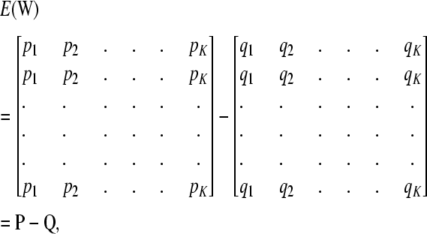and P and Q are matrices whose columns contain p_k and q_k, respectively, in every position of column k. Every element of the column vector is the same and equal to , a constant that can be absorbed into the intercept element of β. Hence, and without loss of generality, .

The covariance matrix (regarding β and marker effects a_m as fixed parameters) is

Here

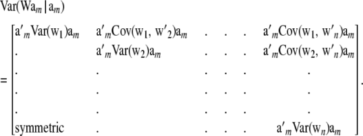If genotypes are drawn at random from the same population, all w_i vectors have the same distribution, that is, for all i. If the population is in HW–LE, is a diagonal matrix. Further, if individuals are genetically related, off-diagonal terms are not null, because of covariances due to genotypic similarity.

To illustrate, let i be a randomly chosen male mated to a random female, and let j be a randomly chosen descendant. Under HW–LE, genotypes at different marker loci are mutually independent, within and between individuals, so it suffices to consider a single locus. It turns out that

yielding the standard result that the covariance between genotypes of offspring and parent is of the variance between genotypes at the locus in question. This generalizes readily to any type of additive relationships in the population.

Letting r_ij be the additive relationship between i and j,

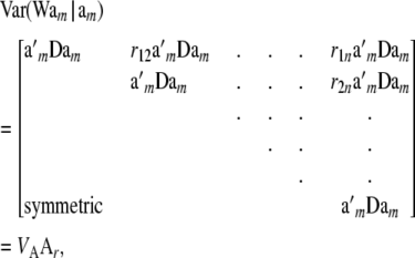(33)

where

(34)

is the additive genetic variance among multilocus genotypes in HW–LE, and is the matrix of additive relationships between individuals; D is diagonal in this case. The variance–covariance matrix (33) involves the fixed marker effects a_m, but these get absorbed into V_A.

The implication is that a model with the conditional (given marker effects and gene frequencies) expectation function

(35)

[recall that ] and conditional covariance matrix

(36)

has the equivalent representation

(37)

with distributed as

(38)

This is precisely the standard model of quantitative genetics applied to a finite number of marker loci (K), where additive genetic variation stems from the sampling of genotypes but not of their effects. The assumption of normality is not required.

Formulas under LD are given in the second section of the appendix.

Estimating the pedigree-based relationship matrix and expected heterozygosity using markers:

Consider model (37):

Given the observed marker genotypes W, the distribution of W is irrelevant with regard to inference about a*. It is relevant only if one seeks to estimate parameters of the genotypic distribution, e.g., gene frequencies and linkage disequilibrium statistics. Consider, for instance, the expected value of WW′:

where , and the sum is over markers. If all individuals belong to the same genotypic distribution, as argued above,

(39)

as in Habier et al. (2007); if , then so . Under this idealized assumption provides an unbiased estimator of the pedigree-based additive relationship matrix, but only if HW–LE holds. Note that under a beta distribution of gene frequencies

Likewise

Using this continuous approximation, (39) becomes

where is the expected heterozygosity. Since the relationship holds for any combination i, j and there are n(n + 1)/2 distinct elements in WW′ and in A_r, one can form an estimator of mean heterozygosity as

where and are averages over all distinct elements in WW′ and A_r. The estimator is simple, but no claim is made about its properties.

CONNECTION WITH THE INFINITESIMAL MODEL

Clearly, (31) or (37) with (38) involves a finite number of markers, and the marked additive genetic variance is a function of allelic frequencies and of effects of individual markers. In the infinitesimal model, on the other hand, the effects of individual loci or of gene frequencies do not appear explicitly. How do these two types of models connect?

The vector of additive genetic effects (or marked breeding value) of all individuals is . Next, assume that effects a₁, a₂, … , a_K are independently and identically distributed as , but this does not need to be so. Again, is not the additive genetic variance, which is given by (34) above.

Assuming implies that a* = Wa_m must be normal (given W). However, the elements of W (indicators of genotypes, discrete) are also random so the finite sample distribution of a* is not normal; however, as K goes to infinity, the distribution approaches normality, as discussed later in this section. If a_m and W are independently distributed, the mean vector and covariance matrix of the distribution of marked breeding values are

(40)

and

(41)

Using the fact that and (33), then under LE assumptions

Since , it follows that

(42)

This shows that when both genotypes (the w's) and their effects (the a's) vary at random according to independent trinomial (at each locus) and normal distributions, respectively, the variance of the distribution of a marked breeding value a* is affected by differences in gene frequencies p_k − q_k, by the variance of the distribution of marker effects , and by the level of heterozygosity. In the special case where allelic frequencies are equal to at each of the loci, the first term vanishes and one gets , where . This can be construed as the counterpart of the polygenic additive variance of the standard infinitesimal model, but in a special situation. Again, this illustrates that σ_a² relates to additive genetic variance in a more subtle manner than would appear at first sight.

What is the distribution of marked breeding values when both w_ik and a_k vary at random? Because a_k is normal, the conditional distribution | w_i is normal, with mean 0 and variance . Thus, one can write the density of the marginal distribution of as

where is the probability of observing the K-dimensional marker genotype w_i in individual i. If the population is in HW–LE at all K marker loci, the joint distribution of genotypes of an individual over the K loci is the product of the marginal distributions at each of the marker loci; that is,

For example, if individual i is AA at locus k, w_ik1 = 1, w_ik2 = 0, and w_ik3 = 0; if i is heterozygote w_ik1 = 0, w_ik2 = 1, and w_ik3 = 0, and if i has genotype aa, then w_ik1 = 0, w_ik2 = 0, and w_ik3 = 1. Note that w_ik3 = 1 − w_ik1 − w_ik2, so that there are only two free indicator variates. It follows that the marginal distribution of is a mixture of 3^K normal distributions each with a null mean, but distribution-specific variance . As , the mixing probabilities become infinitesimally small, so that

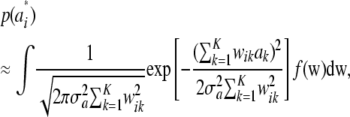for some density f(w). The mixture distribution of must necessarily converge toward a Gaussian one, because is the sum of a large (now infinite) number of independent random variates (note that under LE w_ika_k is independent of any other w_ik′a_k′ because genotypes at different loci are mutually independent), so the central limit theorem holds; it holds even under weaker assumptions. Then

Since all components of the mixture have null means, its variance is just the average of the variances of all components of the mixture (Gianola et al. 2006b); that is,

This is the additive genetic variance of an infinitesimal model, i.e., one with an infinite number of loci, so that the probability of any genotypic configuration is infinitesimally small.

When the joint distribution of additive genetic values a* of a set of individuals is considered, it is reasonable to conjecture that it should be multivariate normal, especially under LE. Its mean vector is , as shown in (40), and the covariance matrix of the limiting process can be deduced from (42). The first term becomes null, because allelic frequencies became infinitesimally small as , so the covariance matrix tends to

As shown by Habier et al. (2007), markers may act as a proxy for a pedigree. Hence, unless the pedigree is introduced into the model in some explicit form, markers may be capturing relationships among individuals, as opposed to representing flags for QTL regions. At any rate, it is essential to keep in mind that markers are not genes.

THE BAYESIAN ALPHABET

The preceding part of this article sets the quantitative genetics theory basis upon which marker-assisted prediction of breeding value (using linear models) rests. Specifically, Meuwissen et al. (2001) use this theory to assess values of hyperparameters of some Bayesian models proposed by these authors. In what follows, a critique of some methods proposed for inference is presented.

Bayes A:

Meuwissen et al. (2001) suggested using model (31) for marker-enabled prediction of additive genetic effects and proposed two Bayesian hierarchical structures, termed “Bayes A” and “Bayes B.” A brief review of these two methods follows, assuming that k denotes a SNP locus.

In Bayes A (using notation employed here), the prior distribution of a marker effect a_k, given some marker-specific uncertainty variance , is assumed to be normal with null mean and dispersion . In turn, the variance associated with the effect of each marker k = 1, 2,…, K is assigned the same scaled inverse chi-square prior distribution , where ν and S² are known degrees of freedom and scale parameters, respectively. This hierarchy is represented as

The marginal prior induced for a_k is obtained by integrating the normal density over , yielding

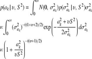(43)

(Box and Tiao 1973; Sorensen and Gianola 2002). This is the kernel of the density of the t-distribution , which is the de facto prior in Meuwissen et al. (2001) assigned to a marker effect. Again, υ, S² are assumed known and given arbitrary values by the user; this is a crucial issue.

Bayes B:

In Bayes B, Meuwissen et al. (2001) proposed

This implies that the joint prior distribution of a_k and , given an arbitrary probability parameter π, is

where c is a constant (if , this implies that a_k is known with certainty), taken by Meuwissen et al. (2001) to be equal to 0, even though it does not need to be 0. Marginally, after integrating out, the prior takes the form

Then, Bayes B reduces to Bayes A by taking π = 0.

A critique:

Neither Bayes A nor Bayes B (or any variations thereof that assume marker-specific variances) allow Bayesian learning on these variances to proceed far away from the prior. This means that the hyperparameters of the prior assigned to these variances (according to assumptions based on quantitative genetics theory) will always have influence on the extent of shrinkage produced on marker effects. A user can arbitrarily control the extent of shrinkage simply by varying υ and S². It suffices to illustrate this problem with Bayes A, since the problem propagates to Bayes B.

It is straightforward to show that the fully conditional (i.e., given all other parameters and the data, a situation denoted as ELSE hereinafter) posterior distribution of is the scaled inverse chi-square process , so Bayesian learning “moves” only a single degree of freedom away from the prior distribution , even though its scale parameter is modified from S² into (most markers are expected to have nearly null effects). Now, since a_k is unknown, and inferring it consumes information contained in the data, this implies that, unconditionally (that is, a posteriori), inferences about are even more strongly affected by the information encoded by its prior distribution than in the conditional posterior process. For instance, if ν = 5, say, this means that the posterior degree of belief about has an upper bound at 6, irrespective of whether data on millions of markers or of individuals become available.

For parameter θ of a model, Bayesian learning should be such that the posterior coefficient of variation, that is, , tends to 0 asymptotically as DATA accrue. This does not happen in Bayes A or Bayes B for . In Bayes A, the coefficients of variation of the prior and of the fully conditional posterior distribution are

and

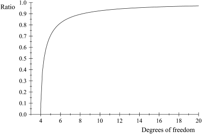
respectively, so that . This ratio goes to 1 rapidly as the degrees of freedom of the prior increase (meaning that the prior “dominates” inference), as illustrated in Figure 1. For example, if ν = 4.1, ν = 5.1, and ν = 6.1, the ratio between the coefficients of variation of the conditional posterior distribution of and that of its prior is ∼0.30, 0.72, and 0.82, so that the prior is influential even at mild values of the degrees of freedom. Given a large ν, the conditional posterior essentially copies the prior, with the contribution of DATA being essentially nil. As mentioned, since marginal posterior inferences about require deconditioning over a_k (thus consuming information contained in the data), the impact of the prior will be even more marked at the margins. This is questionable, at least from an inference perspective.

Figure 1.—

Ratio between coefficients of variation of the conditional posterior and prior distributions of the variance of the marker effect, as a function of the degrees of freedom ν of the prior.

Another way of illustrating the same problem is based on computing information gain, i.e., the difference in entropy before and after observing data. Since the posterior distribution of is unknown, we consider the entropy of the fully conditional posterior distribution of , instead of that of the marginal process. This provides an upper bound for the information gain. The entropy of the prior is

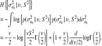(44)

In the entropy of the fully conditional posterior distribution of , , ν is replaced by ν + 1 and νS² by (it is expected that ≈ νS² for most markers). The relative information gain (fraction of entropy reduced by knowledge encoded in ELSE) is then

(45)

For instance, RIG = 1 if the entropy of the conditional posterior process is 0. Assume a nil marker effect and a root-scale parameter S = 1. For a_k = 0, S = 1, and ν = 4, RIG = 0.125; for a_k = 0, S = 1, and ν = 10, then RIG = 6.51 × 10⁻²; and for a_k = 0, S = 1, and ν = 100, RIG = 9.60 × 10⁻³. Even at mild values of the prior degrees of freedom ν, the extent of uncertainty reduction due to observing data is negligible. Metaphorically, the prior is totalitarian in Bayes A, at least for each one of the parameters.

A third gauge is the Kullback–Leibler distance (KL) between the prior and conditional posterior distributions. The KL metric (Kullback 1968) is the expected logarithmic divergence between two parametric distributions, one taken as reference or point of departure. Using the prior as reference distribution, the expected distance is

where

is a randomly varying distance (randomness is due to uncertainty about , and p is the number of markers that are assigned the same variance, so that p = 1 and a_m = a_k in Bayes A; however, p could be much larger if, say, all p markers on the same chromosome were assigned the same variance.

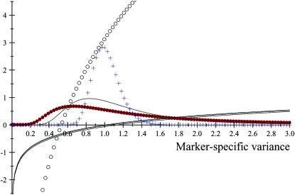
The impact of the degrees of freedom of the prior on the random quantity L(.) of the integrand in KL was examined by assuming that the conditional posterior distribution of had a_k = 0 (again, most marker effects are expected to be tiny, if not null) and that the scale parameter of the prior of the marker-specific variances was S = 1. Figure 2 displays three scaled inverse chi-square densities, all with the same parameter S = 1 and degrees of freedom 4, 10, or 100, as well as values of the random quantity with p = 1 and a_k = 0 in the KL gauge. Also shown in Figure 2 (in open circles) are values of for p = 10, meaning that, instead of having marker-specific variances, 10 markers would share the same variance. While the three priors are different, and reflect distinct states of prior uncertainty about via their distinct degrees of freedom, the values are essentially the same irrespective of and flat for any values of appearing with appreciable density in the priors. On the other hand, if it is assumed that , where is now a variance assigned to a group of markers (even assuming that their effects are nil), is steep with respect to , taking negative values for <0.55 (roughly). In fact, the KL distances (evaluated with numerical integration) between the prior and conditional posterior distributions are (1) 7.33 × 10⁻² for ν = 4, S = 1, p = 1 and a_k = 0; (2) 2.64 × 10⁻² for ν = 10, S = 1, p = 1 and a_k = 0; and (3) 2.52 × 10⁻³ for ν = 100, S = 1, p = 1, and a_k = 0, so that the conditional posterior is very close to the prior even at small values of the degrees of freedom parameter. However, when the number of markers sharing the same variance increases to p = 10 (assuming all 's = 0, as stated), KL = 4.47, so that considerable Bayesian learning about takes place in this situation. Relative to scenario 1 above, the KL distance increases by ∼61 times.

Figure 2.—

Prior densities of the marker-specific variance (solid circles, ν = 4, S = 1; solid curve, ν = 10, S = 1; crosses, ν = 100, S = 1) and values of integrand in the Kullback–Leibler distance, for each of the three priors, shown as solid lines. The integrands are essentially indistinguishable from each other for all values of . Values of the integrand are drastically different (open circles) when 10 markers are assigned the same variance, so that .

A pertinent question is whether or not the learned marker effect (i.e., a draw from its conditional posterior distribution) has an important impact on KL via modification of the scale parameter from S² into . Let be the realized value of the marker effect in units of the “prior standard deviation” S, with c = 0, 0.01, 0.5, 1, and 2; the last two cases would be representative of markers with huge effects. The density of the conditional posterior distribution of is then

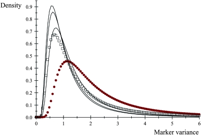
The KL distances between the conditional posterior and the prior for these five situations, assuming S = 1 and ν = 4, are (1) , (2) KL, (3) KL, (4) KL, and (5) KL. Even though marker effects are drastically different, the conditional posteriors are not too different (in the KL sense) from each other, meaning that the extent of shrinkage in Bayes A (or B) continues to be dominated by the prior. This is illustrated in Figure 3: even when c = 2, the conditional posterior does not differ appreciably from the prior.

Figure 3.—

Effect of scale parameter on the conditional posterior distribution of the variance of the marker effect. Open boxes, prior distribution; solid circles, conditional posterior distribution for c = 2 (standardized marker effect). The other three conditional distributions (solid lines) are barely distinguishable from the prior.

In short, neither Bayes A nor Bayes B, as formulated by Meuwissen et al. (2001), allows for any appreciable Bayesian learning about marker-specific variances so that, essentially, the extent of shrinkage of effects will always be dictated strongly by the prior, which negates the objective of introducing marker-specific variances into the model. The magnitudes of the estimates of marker effects can be made smaller or larger at will via changes of the degrees of freedom and scale parameters of the prior distribution.

Arguably, Bayes B is not well formulated in a Bayesian context. Meuwissen et al. (2001) interpret that assigning a priori a value with probability π means that the specific SNP does not have an effect on the trait. As mentioned earlier in this article, stating that a parameter has 0 variance a priori does not necessarily mean that the parameter takes value 0: it could have any value, but known with certainty. Thus, assuming implies determinism about such an effect. It turns out, however, that their sampler sets a_k = 0 when the state is drawn! A more reasonable specification is to place the mixture with a 0 state at the level of the effects, but not at the level of the variances.

Impact on predictions:

A counterargument to the preceding critique could be articulated as follows: Even though the prior affects inferences about marker-specific variances, this is practically irrelevant, because one can “kill” the influence of the prior on estimates of marker effects simply by increasing sample size. Superficially, it seems valid, because the fully conditional posterior distribution of a_k (assuming a model with a single location parameter μ) is

As sample size n increases, tends to so the influence of vanishes asymptotically, given some fixed values of ν, S. This indicates that, in Bayes A, even though Bayesian learning about the parameters is limited, the influence of the prior on the posterior distributions of marker effects and of the genetic values dissipates in large samples. However, in marker-assisted prediction of genetic values n < < p, so the prior may be influential. The sensitivity of Bayes A with respect to the prior in a finite sample was examined by simulation.

Simulation:

Bayes A was fitted under different prior specifications to a simple data structure. Records for 300 individuals were generated under the additive model

where y_i is the phenotype for individual i, and the rest is as before. Residuals were independently sampled from a standard normal distribution.

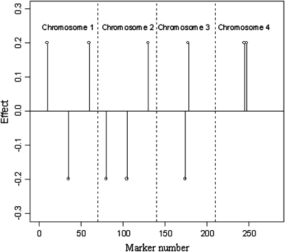
Two LD scenarios regarding the distribution of the 280 markers were generated. In scenario X0, markers were in weak LD, with almost no correlation between genotypes of adjacent markers (Table 1). In scenario X1, LD was relatively high: the correlation between markers dropped from 0.772 for adjacent markers to 0.354 for markers separated by three positions (Table 1). Effects of allele substitutions were kept constant across simulations and were set to zero for all markers except for 10, as shown in Figure 4. The locations of markers with nonnull effects were chosen such that different situations were represented. For example (Figure 4), in chromosome 3 there were two adjacent markers with opposite effects, while chromosome 4 had two adjacent markers with equal effects.

TABLE 1.

Correlation between marker genotypes (average over markers and over 100 Monte Carlo replicates) by scenarios of adjacency between pairs of markers and of linkage disequilibrium (X0, low linkage disequilibrium; X1, high linkage disequilibrium)

	Adjacency	Adjacency	Adjacency	Adjacency
Disequilibrium scenario	1	2	3	4
X0	0.007	0.002	−0.002	0.013
X1	0.722	0.567	0.450	0.356

Figure 4.—

Positions (chromosome and marker number) and effects of markers (there were 280 markers, with 270 having no effect).

A Monte Carlo study with 100 replicates was run for each of the two LD scenarios. For each replicate and LD scenario, nine variations of Bayes A were fitted, each defined by a combination of prior values of hyperparameters. In all cases, a scale inverted chi-square distribution with 1 d.f. and scale parameter equal to 1 were assigned to the residual variance. The nine priors considered are in Table 2. Hyperparameter values were chosen such that the prior had, at most, the same contribution to the degrees of freedom of the fully conditional distribution as the information coming from the remaining components of the model (i.e., 1). Values of S² were chosen following similar considerations. Note that if the samples of marker effects are equal to their true value, ≤ 0.2² (see Figure 4). Priors 1–3 are improper, and the other six priors are proper but do not possess finite means and variances. Therefore, scenarios with S² = 10⁻⁵ correspond to cases of relatively small influence of the prior on the scale parameter of the fully conditional distribution, while S² = 5 × 10² represents a case where the fully conditional distribution has a strong dependency on the prior specification.

TABLE 2.

Nine different specifications of hyperparameters of the prior distribution of marker variances in Bayes A (ν, prior degrees of freedom; S², prior scale parameter)

	S2 = 10−5	S2 = 10−3	S2 = 5 × 102
ν = 0	1	2	3
	4	5	6
ν = 1	7	8	9

For each of these models and Monte Carlo replicates 35,000 iterations of the Gibbs Sampler were run, and the first 5000 iterations were discarded as burn-in. Inspection of trace plots and other diagnostics (effective sample size, MC standard error) computed using Coda (Plummer et al. 2008) indicated that this was adequate to infer quantities of interest.

Table 3 shows the average (across 100 MC replicates) of posterior means of the residual variance and of the correlation between the true and the estimated quantity of several features. This provides an assessment of goodness of fit, of how well the model estimates genomic values, and of the extent to which the model can uncover relevant marker effects. As expected, Bayes A was sensitive with respect to prior specification for all items monitored. Scenarios 4 and 7 produced overfitting (low estimate of residual variance, whose true value was 1, and high correlation between data and fitted values). It also had a low ability to recover signal (i.e., to estimate marker effects and genomic values), as indicated by the corresponding correlations. Other priors (e.g., 6) produced a model with a better ability to estimate genomic values and marker effects. These results were similar in both scenarios of LD. The results in Table 3 also indicate that it is much more difficult to uncover marker effects than to predict genomic values.

TABLE 3.

Average (over 100 replicates) of posterior mean estimates of residual variance (σ²) and of the correlation between the true and the estimated value for several items (phenotypes, y; true genomic value, Wa_m; fitted genomic value, ; true marker effects, a_m; estimated marker effects,

	σ2
	Mean	SD	Mean	SD	Mean	SD	Mean	SD
Low linkage disequilibrium between markers (X0)
Bayes A
1	0.518	0.062	0.839	0.027	0.580	0.063	0.102	0.048
2	0.941	0.089	0.577	0.028	0.721	0.092	0.200	0.022
3	1.074	0.105	0.496	0.032	0.701	0.106	0.199	0.020
4	0.394	0.053	0.895	0.022	0.531	0.060	0.079	0.051
5	0.824	0.077	0.652	0.025	0.699	0.079	0.183	0.028
6	0.950	0.089	0.578	0.027	0.722	0.088	0.201	0.021
7	0.173	0.053	0.966	0.015	0.455	0.057	0.042	0.043
8	0.575	0.056	0.813	0.019	0.606	0.066	0.116	0.044
9	0.710	0.066	0.728	0.020	0.659	0.072	0.152	0.037
High linkage disequilibrium between markers (X1)
Bayes A
1	0.535	0.069	0.824	0.029	0.580	0.070	0.121	0.045
2	0.938	0.076	0.609	0.033	0.677	0.083	0.210	0.026
3	1.093	0.085	0.528	0.034	0.650	0.086	0.211	0.025
4	0.404	0.067	0.888	0.025	0.533	0.067	0.094	0.048
5	0.809	0.069	0.670	0.030	0.659	0.076	0.200	0.030
6	0.948	0.075	0.616	0.031	0.676	0.081	0.211	0.026
7	0.195	0.056	0.960	0.015	0.462	0.060	0.062	0.048
8	0.566	0.058	0.809	0.021	0.593	0.070	0.132	0.042
9	0.689	0.062	0.734	0.024	0.629	0.072	0.173	0.036

SD, among-replicates standard deviation of item.

To have a measure of the ability of each model to locate genomic regions affecting the trait, an index was created as follows. For each marker having a nonnull effect and for each replicate, a dummy variable was created indicating whether or not the marker, or any of its 4 flanking markers, ranked among the top 20 on the basis of the absolute value of the posterior mean of the marker's effect. Averaging across markers and replicates led to an index of “retrieved regions” (Table 4). Results suggest that the ability of Bayes A to uncover relevant genomic regions is also affected by the choice of hyperparameters. For example, in scenarios 1, 4, and 7 only one of five regions was retrieved by Bayes A. On the other hand, the fraction of retrieved regions was twice as large when using other priors (scenarios 2, 3, and 6). The ability to uncover genomic regions affecting a trait was usually worse with high LD, due to redundancy between markers.

TABLE 4.

Fraction of retrieved regions by set of priors in Bayes A and scenario of linkage disequilibrium (LD)

Set of priors in Bayes A	Low LD	High LD
1	0.24	0.21
2	0.43	0.34
3	0.47	0.33
4	0.22	0.19
5	0.36	0.31
6	0.43	0.34
7	0.22	0.18
8	0.26	0.22
9	0.29	0.26

DISCUSSION

This article examined two main issues associated with the development of statistical models for genome-assisted prediction of quantitative traits using dense panels of markers, such as single-nucleotide polymorphisms. The first one is the relationship between parameters from standard quantitative genetics theory, such as additive genetic variance, and those from marker-based models, i.e., the variance of marker effects. In a Bayesian context, the latter act mainly as a measure of uncertainty. It was shown that the connection between the variance of marker effects and the additive genetic variance depends on what is assumed about locus effects. For instance, in the classical model of Falconer and Mackay (1996), locus effects are considered as fixed and additive genetic variance stems from random sampling of genotypes. To introduce a variance of marker effects, these must be assumed to be random samples from some distribution that, in the Bayesian setting, is precisely an uncertainty distribution. The article also discussed assumptions that need to be made to establish a connection between the two sets of parameters and introduced a more general partition of variance, in which genotypes, effects, and allelic frequencies are random variables. Some expressions for relating additive genetic variance and that of marker effects are available under the assumption of linkage equilibrium, as discussed in the article. However, accommodating linkage disequilibrium explicitly into an inferential system suitable for marker-assisted selection represents a formidable challenge.

The second aspect addressed in this study was a critique of methods Bayes A and B as proposed by Meuwissen et al. (2001). These methods require specifying hyperparameters that are elicited using formulas related to those mentioned in the paragraph above; however, the authors did not state the assumptions needed precisely. It was shown here that these hyperparameters can be influential.

The influence of the prior on inferences and predictions via Bayes A can be mitigated in several ways. One way consists of forming clusters of markers such that their effects share the same variance. Thus, shrinkage would be specific to the set of markers entering into the cluster. The clusters could be formed either on the basis of biological information (e.g., according to coding or noncoding regions specific to a given chromosome) or perhaps statistically, using some form of supervised or unsupervised clustering procedure. If clusters of size p were formed, the conditional posterior distribution of the variances of the markers would have p + ν d.f., instead of 1 + ν in Bayes A. A second way of mitigating the impact of hyperparameters is to assign a noninformative prior to the scale and degrees of freedom parameters of Bayes A. This has been done in quantitative genetics, as demonstrated by Strandén and Gianola (1998) and Rosa et al. (2003, 2004) and discussed in Sorensen and Gianola (2002). For example, Strandén and Gianola (1998) used models with t-distributions for the residuals (the implementation would be similar in Bayes A, with the t-distribution assigned to marker effects instead), with unknown degrees of freedom and unknown parameters. In Strandén and Gianola (1998) a scaled inverted chi-square distribution was assigned to the scale parameter of the t-distribution, and equal prior probabilities were assigned to a set of mutually exclusive and exhaustive values of the degrees of freedom. On the other hand, Rosa et al. (2003, 2004) presented a more general treatment, in which the degrees of freedom were sampled with a Metropolis–Hastings algorithm. A third modification of Bayes A would consist of combining the two preceding options, i.e., assign a common variance to a cluster of marker effects and then use noninformative priors, as in Rosa et al. (2003, 2004), for the parameters of the t-distribution. Applications of thick-tailed priors, such as the t or the double exponential distribution, to models with marker effects are presented in Yi and Xu (2008) and de los Campos et al. (2009a).

Bayes B requires a reformulation (and a new letter, to avoid confusion!), e.g., the mixture with a zero state posed at the level of effects and not at that of the variances, as discussed earlier. For example, one could assume that the marker effect is 0 with probability π or that it follows a normal distribution with common variance otherwise. Further, the mixing probability π could be assigned a prior distribution, e.g., a beta process, as opposed to specifying an arbitrary value for π. Mixture models in genetics are discussed, for example, by Gianola et al. (2006b) and some new, yet unpublished, normal mixtures for marker-assisted selection are being developed by R. L. Fernando (R. L. Fernando, unpublished data) (http://dysci.wisc.edu.edu/sglpe/pdf/Fernando.pdf).

A more general solution is to use a nonparametric method, as suggested by Gianola et al. (2006a), Gianola and van Kaam (2008), Gianola and de los Campos (2008) and casted more generally by de los Campos et al. (2009a). These methods do not make hypotheses about mode of inheritance, contrary to the parametric methods discussed above, where additive action is assumed. Evidence is beginning to emerge that nonparametric methods may have better predictive ability when applied to real data (González-Recio et al. 2008, 2009; N. Long, D. Gianola, G. J. M. Rosa and K. A. Weigel, unpublished results.).

In conclusion, this article discussed connections between marker-based additive models and standard models of quantitative genetics. It was argued that the relationship between the variance of marker effects and the additive genetic variance is not as simple as has been reported, becoming especially cryptic if the assumption of linkage equilibrium is violated, which is manifestly the case with dense whole-genome markers. Also, a critique of earlier models for genomic-assisted evaluation in animal breeding was advanced, from a Bayesian perspective, and some possible remedies of such models were suggested.

APPENDIX

Linkage disequilibrium:

The expression results from jointly sampling genotypes (but not their effects) at K loci in linkage equilibrium. This is a needed assumption for arriving at (19). On the other hand, if there is LD, the additive genetic variance (under HW equilibrium at each locus) is

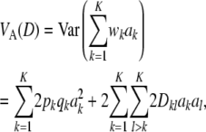(A1)

where p_B,l is the usual LD statistic involving the two loci in question. The first term in (A1) is the additive genetic variance under LE; the second term is a contribution to variance from LD, and it may be negative or positive. It can be shown that the average correlation between genotypes at a pair of loci is (approximately) <K⁻¹.

The average (over a effects) variance under LD depends on the distribution of the a's. If these are independently and identically distributed with mean θ and variance , one has

(A2)

If θ = 0, then (D) = , in which case linkage disequilibrium would not affect relationship (19).

There is no mechanistic basis for expecting that all loci have the same effects and for these being mutually independent. There may be some genomic regions without any effect at all, or some regions may induce similarity (or dissimilarity) of effects; for example, if two genes are responsible for producing a fixed amount of transcript, their effects would be negatively correlated, irrespective of whether or not genotypes are in linkage equilibrium. A more general assumption may be warranted, i.e., that effects follow some multivariate distribution , where is just a dispersion parameter. Here, with w being the vector of genotypes for the K loci, one can write the average variance under LD,

where M is the covariance matrix of w (diagonal under LE),

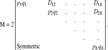Further,

where is the trace of the matrix in question. The counterpart of (19) is

(A3)

which is a complex relationship even if θ = 0. It follows that (19), appearing often in the literature, holds only under strong simplifying assumptions. In short, the connection between additive genetic variance and the variance of marker effects depends on the unknown means of the distributions of marker effects, their possible covariances (induced by unknown molecular and chromosomal process), their gene frequencies, and all pairwise linkage disequilibrium parameters, which are a function of the 's. It is not obvious what the effects of using (19) as an approximation are, but the assumptions surrounding it are undoubtedly strong.

Covariance between relatives and linkage disequilibrium:

Linkage disequilibrium complicates matters, as noted earlier. The covariance between marked genetic values of individuals i and j, instead of being , takes the form

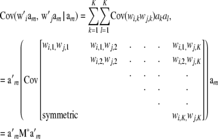and M* is no longer a diagonal matrix, because of LD creating covariances between genotypes at different marker loci. The diagonal elements of M* have the form (assuming HW frequencies within each locus)

and the off-diagonals are

This implies that disequilibrium statistics D must be brought into the picture when estimating a pedigree relationship matrix using markers in LD.

References

- Barton, N. H., and H. P. de Vladar, 2009. Statistical mechanics and the evolution of polygenic quantitative traits. Genetics 181: 997–1011. [DOI] [PMC free article] [PubMed] [Google Scholar]
- Box, G. E. P., and G. C. Tiao, 1973. Bayesian Inference in Statistical Analysis. Addison-Wesley, Reading, MA.
- de los Campos, G., D. Gianola and G. J. M. Rosa, 2009. a Reproducing kernel Hilbert spaces regression: a general framework for genetic evaluation. J. Anim. Sci. 87: 1883–1887. [DOI] [PubMed] [Google Scholar]
- de los Campos, G., H. Naya, D. Gianola, J. Crossa, A. Legarra et al., 2009. b Predicting quantitative traits with regression models for dense molecular markers and pedigrees. Genetics 182: 375–385. [DOI] [PMC free article] [PubMed] [Google Scholar]
- Falconer, D. S., and T. F. C. Mackay, 1996. Introduction to Quantitative Genetics, Ed. 4. Longmans Green, Harlow, Essex, UK.
- Fernando, R. L., and M. Grossman, 1989. Marker-assisted selection using best linear unbiased prediction. Genet. Sel. Evol. 33: 209–229. [Google Scholar]
- Gianola, D., and G. de los Campos, 2008. Inferring genetic values for quantitative traits non-parametrically. Genet. Res. 90: 525–540. [DOI] [PubMed] [Google Scholar]
- Gianola, D., and R. L. Fernando, 1986. Bayesian methods in animal breeding. J. Anim. Sci. 63: 217–244. [Google Scholar]
- Gianola, D., M. Pérez-Enciso and M. A. Toro, 2003. On marker-assisted prediction of genetic value: beyond the ridge. Genetics 163: 347–365. [DOI] [PMC free article] [PubMed] [Google Scholar]
- Gianola, D., R. L. Fernando and A. Stella, 2006. a Genomic assisted prediction of genetic value with semi-parametric procedures. Genetics 173: 1761–1776. [DOI] [PMC free article] [PubMed] [Google Scholar]
- Gianola, D., B. Heringstad and J. Ødegård, 2006. b On the quantitative genetics of mixture characters. Genetics 173: 2247–2255. [DOI] [PMC free article] [PubMed] [Google Scholar]
- Gianola, D., and J. B. C. H. M. van Kaam, 2008. Reproducing kernel Hilbert spaces methods for genomic assisted prediction of quantitative traits. Genetics 178: 2289–2303. [DOI] [PMC free article] [PubMed] [Google Scholar]
- González-Recio, O., D. Gianola, N. Long, K. A. Weigel, G. J. M. Rosa et al., 2008. Nonparametric methods for incorporating genomic information into genetic evaluations: an application to mortality in broilers. Genetics 178: 2305–2313. [DOI] [PMC free article] [PubMed] [Google Scholar]
- González-Recio, O., D. Gianola, G. J. M. Rosa, K. A. Weigel and A. Kranis, 2009. Genome-assisted prediction of a quantitative trait in parents and progeny: application to food conversion rate in chickens. Genet. Sel. Evol. 41: 3–13. [DOI] [PMC free article] [PubMed] [Google Scholar]
- Habier, D., R. L. Fernando and J. C. M. Dekkers, 2007. The impact of genetic relationship information on genome-assisted breeding values. Genetics 177: 2389–2397. [DOI] [PMC free article] [PubMed] [Google Scholar]
- Hayes, B. J., P. J. Bowman, A. J. Chamberlain and M. E. Goddard, 2009. Invited review: genomic selection in dairy cattle: progress and challenges. J. Dairy Sci. 92: 433–443. [DOI] [PubMed] [Google Scholar]
- Heffner, E. L., M. E. Sorrell and J. L. Jannink, 2009. Genomic selection for crop improvement. Crop Sci. 49: 1–12. [Google Scholar]
- Kullback, S., 1968. Information Theory and Statistics, Ed. 2. Dover, New York.
- Lande, R., and R. Thompson, 1990. Efficiency of marker-assisted selection in the improvement of quantitative traits. Genetics 124: 743–756. [DOI] [PMC free article] [PubMed] [Google Scholar]
- Long, N., D. Gianola, G. J. M. Rosa, K. A. Weigel and S. Avendaño, 2007. Machine learning classification procedure for selecting SNPs in genomic selection: application to early mortality in broilers. J. Anim. Breed. Genet. 124: 377–389. [DOI] [PubMed] [Google Scholar]
- Maher, B., 2008. The case of the missing heritability. Nature 456: 18–21. [DOI] [PubMed] [Google Scholar]
- Meuwissen, T. H., B. J. Hayes and M. E. Goddard, 2001. Prediction of total genetic value using genome-wide dense marker maps. Genetics 157: 1819–1829. [DOI] [PMC free article] [PubMed] [Google Scholar]
- Plummer, M., N. Best, K. Cowles and K. Vines, 2008. Coda: output analysis and diagnostics for MCMC. http://cran.r-project.org/web/packages/coda/index.html.
- Rosa, G. J. M., C. R. Padovani and D. Gianola, 2003. Robust linear mixed models with normal/independent distributions and Bayesian MCMC implementation. Biom. J. 45: 573–590. [Google Scholar]
- Rosa, G. J. M., D. Gianola and C. R. Padovani, 2004. Bayesian longitudinal data analysis with mixed models and thick-tailed distributions using MCMC. J. Appl. Stat. 31: 855–873. [Google Scholar]
- Sorensen, D., and D. Gianola, 2002. Likelihood, Bayesian, and MCMC Methods in Quantitative Genetics. Springer, New York.
- Strandén, I., and D. Gianola, 1998. Attenuating effects of preferential treatment with Student-t mixed linear models: a simulation study. Genet. Sel. Evol. 30: 565–583. [Google Scholar]
- Turelli, M., 1985. Effects of pleiotropy on predictions concerning mutation selection balance for polygenic traits. Genetics 111: 165–195. [DOI] [PMC free article] [PubMed] [Google Scholar]
- van Raden, P. M., 2008. Efficient methods to compute genomic predictions. J. Dairy Sci. 91: 4414–4423. [DOI] [PubMed] [Google Scholar]
- van Raden, P. M., C. P. van Tassell, G. R. Wiggans, T. S. Sonstegard, R. D. Schnabel et al., 2009. Reliability of genomic predictions for North American Holstein bulls. J. Dairy Sci. 92: 16–24. [DOI] [PubMed] [Google Scholar]
- Wang, C. S., J. J. Rutledge and D. Gianola, 1993. Marginal inferences about variance components in a mixed linear model using Gibbs sampling. Genet. Sel. Evol. 25: 41–62. [Google Scholar]
- Wang, C. S., J. J. Rutledge and D. Gianola, 1994. Bayesian analysis of mixed linear models via Gibbs sampling with an application to litter size in Iberian pigs. Genet. Sel. Evol. 26: 91–115. [Google Scholar]
- Whittaker, J. C., R. Thompson and M. C. Denham, 2000. Marker-assisted selection using ridge regression. Genet. Res. 75: 249–252. [DOI] [PubMed] [Google Scholar]
- Wright, S., 1937. The distribution of gene frequencies in populations. Proc. Natl. Acad. Sci. USA 23: 307–320. [DOI] [PMC free article] [PubMed] [Google Scholar]
- Yi, N., and S. Xu, 2008. Bayesian Lasso for quantitative trait loci mapping. Genetics 179: 1045–1055. [DOI] [PMC free article] [PubMed] [Google Scholar]
- Xu, S., 2003. Estimating polygenic effects using markers of the entire genome. Genetics 163: 789–801. [DOI] [PMC free article] [PubMed] [Google Scholar]
- Zhang, X. S., and W. G. Hill, 2005. Predictions of patterns of response to artificial selection in lines derived from natural populations. Genetics 169: 411–425. [DOI] [PMC free article] [PubMed] [Google Scholar]