

Abstract
Two models (I and II) for the active site structure of class-I ribonucleotide reductase (RNR) intermediate X in subunit R2 have been studied in this paper, using broken-symmetry density functional theory (DFT) incorporated with the conductor like screening (COSMO) solvation model and with the finite-difference Poisson-Boltzmann self-consistent reaction field (PB-SCRF) calculations. Only one of the bridging groups between the two iron centers is different between Model-I and Model-II. Model-I contains two μ-oxo bridges, while Model-II has one bridging oxo and one bridging hydroxo. These are large active site models including up to the fourth coordination shell H-bonding residues. Mössbauer and ENDOR hyperfine property calculations show that Model-I is more likely to represent the active site structure of RNR-X. However, energetically our pKa calculations at first highly favored the bridging oxo and hydroxo (in Model-II) structure of the diiron center rather than having the di-oxo bridge (in Model-I). Since the Arg236 and the nearby Lys42, which are very close to the diiron center, are on the protein surface of RNR-R2, it is highly feasible that one or two anion groups in solution would interact with the positively charged side chains of Arg236 and Lys42. The anion group(s) can be a reductant, phosphate, sulfate, nitrate, and other negatively charged groups existing in biological environment or in the buffer of the experiment. Since sulfate ions certainly exist in the buffer of the ENDOR experiment, we have examined the effect of the sulfate (SO42-, surrounded by explicit water molecules) H-bonding to the side chain of Arg236. We find that when sulfate interacts with Arg236, the carboxylate group of Asp237 tends to be protonated, and once Asp237 is protonated, the Fe(III)Fe(IV) center in X favors the di-oxo bridge (Model-I). This would explain that the ENDOR observed RNR-X active site structure is likely to be represented by Model-I rather than Model-II.
1. Introduction
Ribonucleotide reductases (RNRs) are aerobic enzymes that catalyze the reduction of ribonucleotides to deoxyribonucleotides providing the required building blocks for DNA replication and repair.1,2 Class-I RNR, found in eukaryotes as well as in some prokaryotes and viruses, consists of a homodimer of two dissimilar protein subunits: R1 and R2 in an α2β2 architecture. The ribonucleotide-to-deoxyribonucleotide reactions occur by a long range radical (or proton-coupled-electron-transfer) propagation mechanism initiated by a fairly stable tyrosine (Tyr122 in E. coli) radical (“the pilot light”). It is the subunit R2 that contains a dinuclear iron cluster which initially generates and stabilizes this tyrosine radical. The subunit R1 contains the substrate binding site, and catalyzes the dehydroxylation of the 2'-hydroxyl group of the ribose ring. Presently, the detailed structure of the active diferric form of R2 which contains the tyrosine radical is not known. This neutral tyrosine radical has been identified in R2 with the oxidized Fe(III)Fe(III) active site and is stable for days at room temperature.1 Once this pilot light goes out, the tyrosine radical is regenerated by a high-oxidation intermediate state of RNR-R2, called X.3-7 A combination of Q band ENDOR (electron-nuclear double resonance) and Mössbauer data on Y122F-R2 indicate the iron centers of X are high spin Fe(III) (S = 5/2) and high spin Fe(IV) (S = 2) sites that antiferromagnetically coupled to give an Stotal = 1/2 ground state.8 The formation of X is complicated involving changes in oxidation state and structural rearrangement with coupled electron and proton transfers. First the resting oxidized diferric met form of R2 (R2ox, see Figure 1)9 is reduced by 2 electrons from a reductase protein to the diferrous form, R2red (see Figure 2).10 Next, a molecular oxygen (O2) binds to the diiron center of R2red, and after internal electron transfers, an additional electron is transferred from Trp48 to one of the iron sites. An Fe(III)Fe(IV) S = ½ center called X, is then kinetically and spectroscopically observed.
Figure 1.

The X-ray active site structure of the oxidized (met) diferric RNR-R2 (R2ox(met)) from E. coli. (PDB code: 1RIB).9
Figure 2.

The X-ray active site structure of the reduced diferrous RNR-R2 (R2red) from E. coli. (PDB code: 1XIK).10
RNR-X has captured the attention of many researchers over the past decade to elucidate its chemical and structural nature.3-8,11-32 In recent years, our group has been studying the properties of a set of active site model clusters for RNR-X using broken-symmetry DFT methods,24-28 and have compared them with the available experimental data, including Mössbauer,8 57Fe, 1H, 17O2, and H2 17O ENDOR,15,17,18 EXAFS (extended X-ray absorption fine structure),16 and MCD (magnetic circular dichroism).19 Based on the detailed analysis and comparisons, we have proposed that the experimentally observed, in particular the ENDOR observed RNR-X active site contains two μ-oxo bridges (O1 and O2 in Figure 3), plus one terminal water (O3) which binds to Fe1(III) (where Fe1 is the iron site closer to Tyr122) and also H-bonds to both side chains of Asp84 and Glu238, and one bidentate carboxylate group from the side chain of Glu115.26 To be consistent with our previous work,26 we will name this structure as Model-I hereafter.
Figure 3.

Our proposed active site structure (Model-I) for RNR-X.26,28
Among the various models we have studied,26 Model-II (Figure 4) differs from Model-I by having a proton on the oxygen labeled O2. That is, Model-II contains one μ-oxo (O1) and one μ-hydroxo (O2H) bridges. We eliminated the possibility of Model-II representing the active site of RNR-X,26 since there are three 17O (O1, O2 and O3) and three 1H (one on O2 and two on O3) hyperfine signals in Model-II, which do not agree with the 1H, 17O2, and H2 17O ENDOR experiments on RNR-X.15,17 Recently, Solomon's group performed Fe(IV)-d-d transition calculations using time-dependent density functional theory (TD-DFT) on the RNR-X models similar to our Model-I and Model-II, and compared with their MCD experiments.32 They found that the assignment of the Fe(IV) d-d transitions in wild-type RNR-X best correlates with the structure Fe(III)(μ-O)(μ-OH)Fe(IV) of Model-II.32
Figure 4.

RNR-X active site Model-II, which differs from Model-I by having a bridging hydroxo on site O2, rather than a bridging oxo.
To see whether Model-I or Model-II is more likely to represent the active site of RNR-X, in addition to comparing the calculated properties with available experiments, we also need to examine which model is energetically more favored. That is, we need to calculate the pKa for bridge O2 in the process of {Model-II(μ-O/μ-OH) → Model-I(2μ-O) + H+}. In our previous study,26 we have predicted this pKa to be 4.02 for Y122F mutant models and 2.51 for wild-type active sites. However, our previous Models-I and II were small, which contained only the first shell residues plus the Tyr122 (or mutant Phe122) side chains.26,28 The explicit bulk protein environment was neglected. The quantum cluster was only embedded in a molecular shaped cavity surrounded by a continuum dielectric medium (conductor-like screening (COSMO)33-36 solvation model). Considering the charged groups in the active site and the H-bonding environment, the dielectric constant for COSMO calculations was set to 80 (as for water),26 which is much higher than the commonly used ε = 4 for protein interior.37-40 Our recent studies show that certain Fe-ligand distances (especially Fe1-N(His118) in Model-I) are strongly influenced by the dielectric constant ε chosen for the COSMO solvation model, while the calculated Mössbauer isomer shift and hyperfine properties change very little with ε.41 The geometry for small Model-I (Figure 4) obtained from ε = 80 is very similar to that of a larger Model-I (containing also second and some third shell H-bonding residue side chains) obtained with ε = 10.41 Therefore, from geometric point of view, ε = 80 is not a bad choice for the solvation environment when studying a small active site model for RNR-X containing mainly the first shell ligands. However, the influence of ε on pKa calculations and how to choose the value of ε for pKa predictions are not well known. Although the dielectric value ε = 4 is commonly used for the protein interior, since this is the value of the dielectric constants of crystalline and polymeric amides42 and dry protein and peptide powders,37-40 many studies show that higher effective dielectric constant values (4-30) for protein interiors are needed in reproducing the pKa values of certain internal ionizable groups.40,43-49
In this paper, we expand our RNR-X models-I and II by including the 2nd, and some 3rd, and 4th shell H-bonding residues and explicit water molecules. To see how the active site properties in such large models will change with the outside dielectric constant, we first geometry optimized the clusters in the COSMO solvation model with different ε of 4, 10, and 20. Then the Mössbauer and hyperfine properties are performed at the optimized geometries. Notice that the RNR-X active site is close to the R2 protein surface, and the Arg236 side chain (included in our current larger X models) is actually on the R2 surface, the continuum dielectric model therefore cannot represent well the uneven protein and solvent environment around the quantum clusters. To predict the relative energies of Model-I and Model-II, and therefore the pKa for bridge O2 more accurately and realistically, we will also perform the finite-difference Poisson-Boltzmann self-consistent reaction field (PB-SCRF)50-55 calculations at the COSMO optimized geometries (obtained from ε = 10). Three dielectric regions are defined in the PB-SCRF calculations: the quantum cluster region (ε = 1), the protein region (ε = 4), and the solvent (water) region (ε = 80). The PARSE56 force field atomic radii and charges are assigned to atoms in the protein field. During PB-SCRF, the RNR-X active site model is computed by DFT calculation in the presence of the protein and solvent reaction field. The reaction field is evaluated from a finite-difference solution to the Poisson-Boltzmann (PB) equation, and self-consistency between the reaction field and the electronic structure of the quantum cluster is achieved by iteration.
2. Large RNR-X Models
Our current large Model-I for the active site of RNR-X is shown in Figure 5. Model-II has the same contents except that the bridging oxo (O2 in Figure 3) is changed to bridging hydroxo ((O2)H in Figure 4). The initial positions of the explicit water molecules and the ligand and residue side chains in Models-I and II are taken directly or modified (for Asp84 and O2) from chain A of the oxidized RNR-R2 (met) diferric (Fe(III)-Fe(III)) X-ray crystal structure (PDB code: 1RIB),9 by breaking the Cβ-Cα, Cγ-Cβ or Cδ-Cγ bonds and adding a linking hydrogen atom along the C-C direction to fill the open valence of the terminal carbon atom.57 The first-shell ligands (Asp84, His118, Glu115, His241, Glu204 and Glu238) and Tyr122 are shown and labeled in Figures 3 and 4. The outer shell residues and water molecules are labeled and the H-bonding interactions are shown in Figure 5.
Figure 5.

Current large model for the active site of RNR-X. Site O2 is a bridging μ-oxo in Model-I. It changes to a bridging hydroxo in Model-II. Asp237 is a 1-. anion.
Model-I in Figure 5 contains 166 atoms with net charge -1. By protonating the bridging site O2, the net charge of Model-II is zero.
3. Computational Methodology
All density functional spin-unrestricted calculations have been performed using the Amsterdam Density Functional (ADF) package.58-60 The parametrization of Vosko, Wilk and Nusair (VWN)61 is used for the local density approximation term, and the OPBE62-64 functional is used for the non-local exchange and correlation terms. OPBE is the combination of Handy's optimized exchange (OPTX)64 and PBE correlation (PBEc) functionals.62,63 This potential in general correctly predicts the spin states for several iron complexes.65-67 We have applied this potential in our methane monooxygenase (MMO) intermediates Q and P studies.68,69 Very recently,41 we also used OPBE in studying the quantum cluster size and solvent polarity effects on the geometries and Mössbauer properties of smaller RNR-X Model-I (without Arg236) calculations, and compared with our previous PW9170 calculations.26
Our previous calculations show that site Fe1, which is the iron closer to Tyr122, should be the Fe(III) site in X.26 In the current study, we will only perform calculations on the Fe1(III)Fe2(IV) high-spin antiferromagnetically (AF) coupled { S1 = 5/2, S2 = 2, Stotal = ½} state for both Model-I and Model-II clusters. Usually the AF spin-coupled state cannot be obtained directly from the normal DFT calculations in ADF. As in previous work, we represent the AF spin-coupled state in DFT by a “broken-symmetry” (BS) state,71-73 where a spin-unrestricted determinant is constructed in which one of the Fe site has spin-up electrons as majority spin and the other site has spin-down electrons. To obtain this broken-symmetry solution, first we construct a ferromagnetically (F) spin-coupled (Stotal = 9/2 for X) determinant, where the spins on both irons are aligned in a parallel fashion. Then we rotate the spin vector located on either atom Fe1 or atom Fe2 by interchanging the α and β fit density blocks on site Fe1 or Fe2 from the output file TAPE21 created by this F-coupled calculation in ADF. Using the modified TAPE21 as a restart file and reading the starting spin density from there, we then obtain the expected BS state through single-point energy calculation or geometry optimization.
3.1. Geometry Optimization
Model-I and Model-II are optimized within the COSMO solvation model with ε = 4, 10, and 20, respectively. The triple-ζ polarization (TZP) Slater-type basis sets with frozen cores (C(1s), N(1s), O(1s) and Fe(1s,2s,2p) are frozen) are applied for geometry optimizations. The linking H atoms on Tyr122, Gln43, Trp48, Trp111, Arg236, and Asp237 are fixed during the optimizations.
3.2. Mössbauer Isomer Shift and Quadrupole Splitting Calculations
After geometry optimization, a high-spin F-coupled single-point energy calculation (in COSMO) with all-electron TZP Slater-type basis sets (i.e. without frozen core approximation) is performed at the BS optimized geometry. Its TAPE21 file is then modified by interchanging the α and β fit density blocks on site Fe2. Starting from the modified TAPE21, a BS state single-point energy calculation in COSMO again with all-electron TZP Slater-type basis sets is then performed to obtain the electron density (r(0)) and the electric field gradient (EFG) at the Fe nucleus, the hyperfine A-tensors, and the BS state energy EBS.
The Mössbauer isomer shifts δ are calculated based on ρ(0):
| (1) |
In our previous studies,68,74 the parameters α and C have been fitted separately for the Fe2+,2.5+ and Fe2.5+,3+,3.5+,4+ complexes for PW91, OPBE, and OLYP, with all-electron TZP Slater type basis sets. For the Fe2.5+,3+,3.5+,4+ complexes, we have obtained A = 11877.0, α = -0.312, and C = 0.373 mm s-1 for OPBE potential.
For calculating the Mössbauer quadrupole splittings (ΔEQ), the EFG tensors V are diagonalized and the eigenvalues are reordered so that |Vzz| ≥ |Vxx| ≥ |Vyy|. The asymmetry parameter η is defined as
| (2) |
Then the ΔEQ for 57Fe of the nuclear excited state (I = 3/2) can be calculated as
| (3) |
where e is the electrical charge of a positive electron, Q is the nuclear quadrupole moment (0.15 barns) of Fe.75
3.3. Hyperfine A-tensor Calculations
The ligand 57Fe, 1H, and 17O hyperfine coupling constants are predicted based on the A-tensor calculations in ADF, which assumes that there is only one unpaired electron in the system when the total spin Stotal = ½ and z component Ms = ½.. The spin-orbit coupling contributions to the A-tensors are neglected. For the present systems with high spin AF coupled sites, we therefore need to rescale the ADF-obtained A-tensors by the spin projection coupling factors |KA/2SA| for Fe(III) (KA = 7/3, SA = 5/2) and |KB/2SB| for Fe(IV) (KB = -4/3, SB = 2).25,76,77 Absolute values of the coupling factors are used here, since the broken symmetry state carries the proper A-tensor sign. For the two bridging oxo atoms, the coupling factor is taken as the average of |KA/2SA| and |KB/2SB|.
3.4. Poisson-Boltzmann Self-consistent Reaction Field (PB-SCRF) Calculations
In order to consider both the protein and solvent effects, and therefore obtain the active site energies and hence the pKa values more accurately, DFT/PB-SCRF calculations are performed at the COSMO optimized geometries (obtained with ε = 10) of both Models-I and II. The DFT/PB-SCRF procedure is described briefly as follows. 1) A gas-phase BS state DFT single-point energy calculation is performed at the COSMO-optimized geometry. 2) The CHELPG algorithm78 combined with singular value decomposition79 are then used to fit the point charges of each atom (charges for the linking H atoms are set to zero) from the molecular electrostatic potentials (ESP) calculated by ADF. 3) The interaction energy of the active site Model-I or Model-II (ε = 1) with the protein (ε = 4) and solvent (ε = 80) environment is estimated by solving the Poisson-Boltzmann equation with a numerical finite-difference method using the MEAD 2.2.0 (Macroscopic Electrostatics with Atomic Detail) program developed by Bashford.80-83 The PARSE56 force field atomic radii and charges are assigned to atoms in the protein field. 4) The reaction field plus protein field potential obtained from step 3 is then added to the Hamiltonian of the DFT single-point energy calculation. The iteration of 1 - 4 continues until self-consistency between the reaction field potential and the electronic structure of solute is achieved. Our current DFT/PB-SCRF code is still a serial version. For reducing the computing time, we used the same frozen core TZP basis sets as in geometry optimizations.
In COSMO, charge fit and MEAD calculations, the van der Waals radii for atoms Fe, C, O, N, and H were taken as 1.5, 1.7, 1.4, 1.55, and 1.2 Å, respectively.
3.5. pKa Calculations
To examine whether Model-I or Model-II is energetically more favored, we need to calculate the pKa value for the bridging site O2.
In general, for the following process (M represents “Model”),
| (4) |
the pKa value for the protonated group can be calculated by
| (5) |
For calculating the pKa of site O2, E[M(non-protonated)] and E[M(protonated)] represent the energies of Model-I and Model-II, respectively. If the energies are from COSMO calculations, the final BS energies of the all-electron TZP single-point energy calculations are used here. ΔGsol(H+,1atm) is the solvation free energy of a proton at 1 atm pressure. We will use -263.98 kcal/mol84-86 for this term since so far it is the best measured value (note that previously we have used -262.11 kcal/mol which was obtained from experimental and theoretical analysis26). E(H+) = 12.6416 eV is the calculated energy of a spin restricted proton obtained from gas-phase OPBE calculation. The translation entropy contribution to the gas-phase free energy of a proton is taken as -TΔSgas(H+) = -7.76 kcal/mol at 298 K and 1 atm pressure.87 Finally, for better estimating the zero point energy difference term ΔZPE, we performed gas-phase geometry optimizations and frequency calculations on the small active site Models-I and II, which include the first-shell ligands shown in Figures 3 and 4 and the second-shell water molecules W520 and W621 (see Figure 5). Other second-shell residues Tyr122, Asp237, and Gln43 are replaced by water molecules keeping the H-bonding interactions with the first-shell residues. We then obtained ΔZPE = -7.29 kcal/mol for calculating the pKa of the bridging hydroxyl group for the process of (Model-II → Model-I + H+).
In order to examine how well the OPBE potential and the parameters mentioned above reproduce the known pKa values of simple systems, we have performed pKa calculations for hydrated Fe2+ and Fe3+ cations. The models (Figures S1 and S2), more detailed results (Table S1), and the Cartesian coordinates of the optimized geometries are given in the Supporting Information. Fe2+(Fe3+) and Fe2+(Fe3+)-OH- are surrounded by three layers (42 and 41, respectively) of water molecules. Geometries were optimized with OPBE potential and all-electron TZP Slater-type basis sets in COSMO solvation model with ε = 80. DFT/PB-SCRF calculations were also performed on these optimized geometries. The experimental pKa values of Fe2+ and Fe3+ in aqueous solution were reported as 9.588 and 2.2,89 respectively. Our calculated pKa for Fe(H2O)422+ → Fe(OH)(H2O)41+ + H+ is 10.91 using COSMO energies, and 10.52 with DFT/PB-SCRF energies. For Fe(H2O)423+ → Fe(OH)(H2O)412+ + H+, the calculated pKa's are 1.04 and 1.02, obtained with COSMO and DFT/PB-SCRF, respectively. Both COSMO and DFT/PB-SCRF solvation models yield similar energetic properties for these systems. The calculated pKa's all agree with experiment very well.
4. Results and Discussion
4.1. Calculated Properties of Models I and II
The calculated Fe-Fe and Fe-ligand distances (Å), pKa values, net spin populations (NSP), isomer Shifts δ (mm s-1), Quadrupole Splittings ΔEQ (mm s-1) for large Models I and II obtained within COSMO solvation model with ε = 4, 10, and 20, respectively, in the Fe1(III)Fe2(IV){S1 = 5/2, S2 = 2, Stotal = ½} state are given in Table 1.
Table 1.
Geometries (Å), Isomer Shifts δ (mm s-1), Quadrupole Splittings (ΔEQ) (mm s-1), η, Net Spin Populations (NSP), Broken-Symmetry State Energies (EBS) (-1018 eV), and pKa Values of the Bridging oxygen O2, for Large RNR-X Active Site Models I and II (Figure 5) Optimized within COSMO Solvation Model with ε = 4, 10, and 20, in the Fe1(III)Fe2(IV){S1 = 5/2, S2 = 2, S2 = 2, Stotal = ½} State, and Compared with Experiment (Exp).
| Model-I |
Model-II |
Exp |
|||||
|---|---|---|---|---|---|---|---|
| ε = 4 | ε = 10 | ε = 20 | ε = 4 | ε = 10 | ε = 20 | ||
| Geometry | |||||||
| Fe1-Fe2 | 2.779 | 2.784 | 2.785 | 2.968 | 2.966 | 2.966 | 2.5 |
| Fe1-O1 | 1.936 | 1.933 | 1.932 | 1.934 | 1.934 | 1.937 | |
| Fe2-O1 | 1.733 | 1.732 | 1.732 | 1.706 | 1.706 | 1.705 | |
| Fe1-O2 | 1.951 | 1.958 | 1.959 | 2.168 | 2.164 | 2.161 | |
| Fe2-O2 | 1.744 | 1.750 | 1.750 | 1.948 | 1.948 | 1.950 | |
| Fe1-O3 | 2.125 | 2.135 | 2.135 | 2.077 | 2.087 | 2.092 | |
| Fe1-N-His118 | 2.396 | 2.366 | 2.362 | 2.189 | 2.184 | 2.177 | |
| Fe2-N-His241 | 2.187 | 2.177 | 2.174 | 2.149 | 2.140 | 2.144 | |
| Fe1-O-Asp84 | 2.110 | 2.118 | 2.120 | 2.020 | 2.020 | 2.017 | |
| Fe1-O-Glu115 | 2.000 | 1.996 | 1.996 | 1.979 | 1.967 | 1.976 | |
| Fe2-O-Glu115 | 2.588 | 2.578 | 2.575 | 2.409 | 2.410 | 2.409 | |
| Fe2-O-Glu204 | 2.001 | 2.001 | 2.001 | 1.924 | 1.924 | 1.924 | |
| Fe2-O-Glu238 | 2.098 | 2.102 | 2.105 | 2.010 | 2.015 | 2.014 | |
| δ(Fe1) | 0.55 | 0.55 | 0.55 | 0.52 | 0.52 | 0.52 | 0.56(3) |
| δ(Fe2) | 0.22 | 0.22 | 0.22 | 0.29 | 0.29 | 0.29 | 0.26(4) |
| ΔEQ(Fe1) | -0.41 | -0.36 | -0.36 | 0.69 | 0.66 | 0.64 | -0.9(1) |
| ΔEQ(Fe2) | -0.36 | -0.34 | -0.34 | -0.57 | -0.57 | -0.58 | -0.6(1) |
| η(Fe1) | 0.86 | 0.73 | 0.73 | 0.62 | 0.66 | 0.71 | 0.5(2) |
| η(Fe2) | 0.62 | 0.55 | 0.54 | 0.48 | 0.42 | 0.42 | 2.7(3) |
| NSP(Fe1) | 4.02 | 4.03 | 4.03 | 4.08 | 4.08 | 4.08 | |
| NSP(Fe2) | -3.21 | -3.21 | -3.21 | -3.26 | -3.26 | -3.26 | |
| EBS | -0.189 | -1.323 | -1.720 | -0.369 | -1.181 | -1.416 | |
| pKa(O2{II → I + H+}) | 13.23 | 7.80 | 5.08 | ||||
The net spin populations are the main indication of the high-spin or intermediate-spin character of the Fe sites. In the ideal ionic limit, the net unpaired spin populations are 5 and 4 for the high-spin Fe(III) (five d-electrons) and Fe(IV) (four d-electrons) sites, respectively. The absolute calculated net spins in Table 1 for Models I and II are only smaller by about 1e- than the ionic limit, indicating that the expected oxidation states of the Fe sites with substantial Fe-ligand covalency are correctly predicted. The opposite signs for the spin densities of Fe1 and Fe2 confirm the AF-coupling.
Unlike the small X model (Figure 3) recently studied,41 the Fe-Fe and Fe-ligand distances in the large Models I and II are very stable. Except for Fe1-N-His118, all other Fe-ligand distances differ by less than 0.01 Å when the dielectric constant of the continuum medium changes from 4 to 10 and to 20 in both optimized Models I and II. The largest change happens to the Fe1-N-His118 distance in Model-I, which is shortened by 0.03 Å when ε increases from 4 to 10. This trend was also observed in small Model-I (Figure 3) where this distance decreases sharply with increasing solvent polarity all the way from ε = 4 to ε = 80.41 For current large model-I, this distance is essentially converged when ε > 10.
A very short Fe-Fe distance (2.5 Å) for RNR-X was reported by EXAFS measurements and analysis.16 Model-I with two μ-oxo bridges yields 2.78 Å for the Fe-Fe distance, which is much shorter than that of Model-II (2.97 Å) and closer to the EXAFS data.
As observed in smaller Model-I calculations,41 the calculated Mössbauer isomer shifts are determined mainly by the first shell Fe-ligand interactions, and are rarely (< 0.01 mm s-1) changed with the polarity of the environment for current large Models I and II. Our recent Mössbauer property calculations on the smaller Model-I structures (Figure 3, and models including further H-bonding residues and water molecules shown in Figure 5 but without Arg236) in different dielectric environment (ε = 4, 10, 20, and 80) yield the isomer shifts δ(Fe1) = 0.55 (or 0.54) mm s-1 and δ(Fe2) = 0.23 (or 0.22) mm s-1. Our previous PW91 calculations on small Model-I (with ε = 80) predicted that δ(Fe1) = 0.57 and δ(Fe2) = 0.22 mm s-1.26 All these are almost the same as the current large Model-I results of δ(Fe1) = 0.55 and δ(Fe2) = 0.22 mm s-1), and are very consistent with the experimental observations (0.56±0.03 and 0.26±0.04 mm s-1).8
Previous PW91 calculated isomer shifts for a small Model-II are δ(Fe1) = 0.48 and δ(Fe2) = 0.27 mm s-1,26 where δ(Fe1) is much less than the experimental value (0.56±0.03 mm s-1) and worse than the prediction for Model-I (0.57 mm s-1). However, our current OPBE calculations for large Model-II yield δ(Fe1) = 0.52 and δ(Fe2) = 0.29 mm s-1, which also fall in the range of the experimental data.
The average error of our Mössbauer quadrupole splitting predictions is around 0.3 mm s-1.74 The sign of the quadrupole splitting is also difficult to predict. It may vary with the quantum cluster size, the solvation environment, the calculation methods and the chosen atomic basis sets. We therefore mainly focus on the absolute values of the quadrupole splittings when comparing our calculations with experiment. The absolute values of the observed quadrupole splittings for RNR-X are |ΔEQ(Fe1)| = 0.9±0.1 mm s-1 and |ΔEQ(Fe2)| = 0.6±0.1 mm s-1.8 Our previous PW91 calculations predicted that |ΔEQ(Fe1)| (0.53 mm s-1) is larger than |ΔEQ(Fe2)| (0.23 mm s-1) by 0.3 mm s-1 in Model-I, and |ΔEQ(Fe1)| (0.33 mm s-1) is much smaller than |ΔEQ(Fe2)| (0.71 mm s-1) in Model-II. Therefore, the PW91 calculations show that the predicted Mössbauer isomer shifts and quadrupole splittings of Model-I are better than Model-II in reproducing the corresponding experimental data. Our current OPBE calculations predict the correct order of |ΔEQ(Fe1)| > |ΔEQ(Fe2)| for both Models I and II. However the predicted values of |ΔEQ(Fe1)| and |ΔEQ(Fe2)| are very similar to each other in all dielectric conditions. The difference between |ΔEQ(Fe1)| and |ΔEQ(Fe2)| for Model-II is larger than Model-I. Therefore, current OPBE Mössbauer isomer shift and quadrupole splitting calculations cannot rule out the possibility of Model-II representing the active site of RNR-X.
Next we will compare the energetic properties of these two RNR-X models. Our previous calculated pKa of the bridging oxygen O2 (see Figures 3-5) for the process{Model-II → Model-I + H+} was 2.51 for the wild type active site and 4.02 for the Y122F mutant form,26 which were obtained using COSMO energies with ε = 80.0. In current study, we see although the geometric structures of the large models I and II are stable, their relative electronic energies from COSMO calculations vary with changes in the polarity of the environment. Model-I with net charge -1 is more stabilized in polar solvent (the charge of the diiron di-oxo cluster including only first shell ligands is also -1). The pKa of site O2 is predicted to be 13.23, 7.80, and 5.08 in the continuum medium with ε = 4, 10, and 20, respectively. Therefore, in a nonpolar environment, Model-II with a hydroxo bridge in site O2 and oxo at O1 is energetically more favored. Conversely Model-I with a di-μ-oxo bridge is the more stable protonation state in a polar environment (ε > 10).
Now the question arises whether Model-I or Model-II is more favored in the real protein and solvent (water) environment. No current theoretical method can fully mimic the real biological environment around the RNR-X active site models. Although not perfect, the DFT/PB-SCRF calculations reasonably include the interactions between the active site model cluster and the protein and solvent fields. Since the COSMO optimized geometries of the large active site models with different dielectric constants are very similar, we performed the DT/PB-SCRF calculations on the geometries of Models I and II which were optimized in COSMO with ε = 10. The corresponding results for energies are given in Table 2. Actually our test calculations of DFT/PB-SCRF for a given model geometry optimized using different dielectric constants show very similar solvation energies. The final gas-phase electronic energy (EBS in broken-symmetry state) of Model-I is much higher than Model-II. However, the reaction field energy favors the Model-I active site. The protein field energies are very similar for Models I and II. Overall, the DFT/PB-SCRF calculated pKa for bridging site O2 is 15.01, which shows that the active site Model-II for X with one μ-oxo and one μ-hydroxo bridges is energetically more stable than Model-I with two μ-oxo bridges in the protein and water environment. This DFT/PB-SCRF predicted pKa value is closer to the one (13.23) predicted using the COSMO calculated energies with ε = 4. This may indicate that ε = 4 better represents the dielectric medium around the O2 site. This is reasonable since the protein dielectric constant ε = 4 is used in the DFT/PB-SCRF model, and the protein/water interface is farther away (Figure 5). Note that in RNR-X active site, the polar groups which are directly H-bonding to the first shell ligands mainly locate on the same side as His118 and His241 (Figure 5). Therefore, without including these polar groups and water molecules, the small X model (Figure 3) optimized in COSMO with ε = 4 yields poor geometry for the diiron center (especially for the distance of Fe1-N-His118).41 A much larger dielectric constant (no less than 20) is needed for the small X model to obtain equivalent geometry of larger models which are optimized with low (e = 4) dielectric constant.41 Now in current large X models, these main polar groups are explicitly included in the quantum cluster. Although the side chain of Arg236 is on the RNR-R2 protein surface and the polarity outside Arg236 should similar to water solution, the solvation effect on site O2 by the region outside Arg236 is screened because of the long distance (11 Å). The main solvation effect around site O2 should come from the dielectric medium in the vicinity of O2. No explicit water molecules were found around the O2 site in both the oxidized and reduced RNR-R2 X-ray crystal structures (unlike methane monooxygenase74,90). The side chain of Phe208 and the Cβ-Cγ groups of Gln87 are about 3 Å away from site O2 (see Figure 6, coordinates of Phe208 and Gln87 are taken from the R2 oxidized (met) crystal structure9). Therefore in this specific case, ε = 4 better describes the dielectric medium around O2. Choosing the value of the dielectric constant of a continuum model for the surroundings when studying metalloprotein active site properties is a problem with no simple answer. The solution depends on the size of the quantum cluster model, the specific properties studied, and the position of the active site in the protein. In a word, it is case dependent, and attention has to be paid in analysing relative energies of the active site models without considering the explicit protein environment.
Table 2.
DFT/PB-SCRF Calculations at the COSMO (with ε = 10) Optimized Geometries of Models I and II.
| Model-I | Model-II | |
|---|---|---|
| EBSa | -1007.148 | -1008.786 |
| Eproteinb | -22.69 | -22.24 |
| Ereactionc | -119.80 | -89.07 |
| Etotald | -1013.327 | -1013.613 |
| pKa(O2{II → I + H+}) | 15.01 |
Gas-phase broken-symmetry energy (eV) in the end of the PB-SCRF cycle.
Protein field energy (kcal mol-1).
Reaction field energy (kcal mol-1).
Etotal = EBS + Eprotein + Ereaction (eV).
Figure 6.

The relative positions of the diiron center and the side chains of Phe208 and Gln87.
In conclusion, for the current energetic and pKa calculations, Model-II of RNR-X appears more stable than Model-I and should be favored in representing the active site structure of RNR-X. This is consistent with the conclusion of Solomon's group based on their Fe(IV)-d-d transition calculations.32
However, a dilemma now appears. The CW and pulsed Q-band 1,2H ENDOR measurements only showed two proton signals which were associated with either a terminal water or a 2-fold disordered terminal hydroxo bound to Fe(III).15 The observed 1,2H ENDOR hyperfine signals are nearly axial, consistent only with terminal HXO, not with bridging hydroxo. Our calculated 1H, 17O, and 57Fe A-tensors for both Models I and II are given in Table 3. Since changing the dielectric constant in the COSMO model shows little influence on the calculated A-tensor values, we only present the results calculated with ε = 4 in COSMO model. The predicted 1H A-tensors for the two protons (Ht2 and Ht2) on the terminal water are in very good agreement with the experimental data for both Models I and II. The A-tensor of the third proton (Hbr) on the bridging O2 site of Model-II is very rhombic and very different from the terminal tensors.
Table 3.
Calculated Hyperfine Coupling Constants (MHz) for E. coli RNR-R2-X Active Site Models I and II in Fe1(m)Fe2(IV){S1 = 5/2, S2 = 2, Stotal = ½} State Obtained with Dielectric Constant ε = 4.0, and Compared with Experimental Results.a
| Model-I | Model-II | Exp. | ||||||
|---|---|---|---|---|---|---|---|---|
| Proton hyperfine coupling constants | ||||||||
| Ht1b |
Ht2b |
Ht1 |
Ht2 |
Hbr |
Ht1 c |
Ht2 c |
||
| A1 | -11.39 | -11.62 | -11.05 | -13.04 | -23.30 | -10.25 | -8.8 | |
| A2 | -6.35 | -7.50 | -6.54 | -7.21 | -1.15 | -10.25 | -8.8 | |
| A3 | 18.59 | 16.44 | 20.36 | 17.40 | 16.80 | 20.5 | 17.6 | |
| Aiso | 0.29 | -0.89 | 0.92 | -0.95 | -2.55 | 0.0 | 0.0 | |
| 17O hyperfine coupling constants | ||||||||
| O1 |
O2 |
O3 |
O1 |
O2 |
O3 |
Obrd |
Otd |
|
| A1 | 12.65 | 12.85 | -13.11 | 7.91 | -4.18 | -15.84 | -0.0(10) | -17.0(5) |
| A2 | -17.46 | -17.76 | -15.26 | -8.91 | -6.20 | -20.02 | -22.5(5) | -20.5(5) |
| A3 | -26.15 | -28.16 | -29.36 | -26.51 | -25.39 | -34.75 | -23.5(5) | -34.0(5) |
| Aiso | -10.32 | -11.02 | -19.24 | -9.17 | -11.93 | -23.54 | -15.3 | -23.8 |
| A1aniso | 22.97 | 23.87 | 6.13 | 17.08 | 7.75 | 7.70 | 15.3 | 6.8 |
| A2aniso | -7.14 | -6.74 | 3.98 | 0.26 | 5.73 | 3.52 | -7.2 | 3.3 |
| A3aniso | -15.83 | -17.14 | -10.12 | -17.34 | -13.46 | -11.21 | -8.2 | -10.2 |
| 57Fe hyperfine coupling constants | ||||||||
| Fe1 |
Fe2 |
Fe1 |
Fe2 |
Fe(III)e |
Fe(IV)e |
|||
| A1 | -46.46 | 5.16 | -42.27 | 10.78 | -74.2(2) | 27.5(2) | ||
| A2 | -43.72 | 18.35 | -37.97 | 29.58 | -72.2(2) | 36.8(2) | ||
| A3 | -45.94 | 17.37 | -39.70 | 17.79 | -73.2(2) | 36.8(2) | ||
| Aiso | -45.37 | 13.63 | -39.98 | 19.39 | -73.2 | 33.7 | ||
| A1aniso | -1.09 | -8.47 | -2.29 | -8.61 | -1.0 | -6.2 | ||
| A2aniso | 1.65 | 4.72 | 2.01 | 10.19 | 1.0 | 3.1 | ||
| A3aniso | -0.57 | 3.74 | 0.28 | -1.60 | 0.0 | 3.1 | ||
DFT-calculated A-tensors were rescaled by the spin coupling factors (see text). Aiso represents the isotropic A-tensor, and Aansio stands for the anisotropic A-tensor component. Values in brackets correspond to standard experimental error.
Ht1 is the proton on the terminal (t) water which H-bonds to Glu238, and Ht2 is another proton H-bonding to Asp84.
From Ref. 15.
From Ref. 17. The relative signs of the 3 principal values were determined in the 17O2 and H2 17O ENDOR experiments, but the absolute signs are not known. We have set the signs according to our calculations, respecting the relative signs set by experiment. We also reordered the A-tensor components for convenience so that |A3| is largest.
From Ref. 8.
Further, only one bridging (Obr) oxo 17O signal was found in the 17O2 ENDOR experiment.17 As observed in our small Model-I calculations,26 the calculated A-tensor principal values and principal axes of the two bridging oxo atoms (O1 and O2) in the current large Model-I are also very close to each other, which may explain the single Obr signal observed in 17O2 ENDOR experiment.26 On the other hand, the calculated A-tensors (including orientations) of O1 and O2 in Model-II are different from each other. Therefore, if Model-II represents the active site of RNR-X, the 17O2 and H217O ENDOR experiments should show three distinct signals.
In Table 3 we also present both the calculated and experimental 57Fe hyperfine data. The observed 57Fe hyperfine from ENDOR and magnetic Mössbauer spectroscopies show highly isotropic hyperfine for the high-spin Fe1(III) site and moderate anisotropy for the high-spin Fe2(IV) site. It is very difficult to calculate the isotropic hyperfine coupling constants (Aiso) of metal centers. However, the 57Fe anisotropic components (Aaniso) can be more accurately predicted by the DFT calculations.26,41 Our predicted Aaniso values for the current large Model-I also agree very well with the corresponding experimental ones. The predicted Aaniso's for Model-II deviate more from the observed data, similar to our previous small model calculations.26
Overall, our hyperfine A-tensor calculations favor Model-I over Model-II as the candidate for the X active site structure observed in the ENDOR experiments. However, as discussed above, Model-II is energetically more stable than Model-I in the protein plus solvent environment. Now the question becomes: how can we solve this dilemma?
4.2. Will Explicit Water Molecules around O2 Alter the pKa?
Unlike the X-ray structure of the oxidized differic methane monooxygenase active site,90 where three water molecules were found in the vicinity of site O2,74 as mentioned earlier, no explicit water molecules were found in both the oxidized and reduced RNR-R2 X-ray crystal structures. However, water molecules may exist around O2 in RNR-X state and have an impact on the pKa of O2. We therefore added three water molecules (see Figure 7) between O2 and Asp84 in the similar relative positions of the water molecules found in the differic methane monooxygenase active site.
Figure 7.

Three explicit H-bonding water molecules were added between site O2 and Asp84 in Model-I (upper) and Model-II (lower), in order to examine whether these water molecules will change the acidity of O2. The outer-shell residues and water molecules are the same as in Figure 5.
The geometries of the two models were optimized using COSMO with ε = 4. The Cartesian coordinates of these two optimized geometries are given in the Supporting Information. The broken-symmetry state energy difference between the two models E[Model-I] - E[Model-II] = 4.62 kcal mol-1 is obtained. Therefore, the pKa of site O2 for the process of {Model-II → Model-I + H+} is 13.56, which is about the same as 13.23 obtained for the models without the three explicit water molecules around O2. These water molecules, therefore, did not change the acidity of site O2.
In general, we notice that Model-II has net charge zero. Similarly if a carboxylate group near the active site center is protonated, then Model-I also becomes neutral, and the bridging site O2 may be most stable in the deprotonated state. In another words, the RNR-X active site which is observed by the ENDOR experiments may be Model-I modified by protonating a nearby carboxylate group. Next we will examine if this idea is correct.
4.3. Models I and II with Protonated Asp237
A likely candidate for the residue that can be protonated in our large X model is Asp237. The carboxylate group of Asp237 can be protonated in different ways. To minimize the number of possible calculations and to get an idea how the protonated state of Asp237 will influence the pKa of the bridging site O2, we simply moved the proton on Water727 to the oxygen atom of Asp237 in both Models I and II. The transferred proton is in turn H-bonding to the oxygen atom of Water727. An extra proton was then added to form a new Water727. Figure 8 shows the protonated Asp237 region in both Model-I and Model-II. The new models with protonated Asp237 will be named Model-I-Asp237H and Model-II-Asp237H hereafter. These structures are also geometry optimized in COSMO solvation model with ε = 4, 10, and 20, respectively. The DFT/PB-SCRF calculations are then performed at the COSMO (with ε = 10) optimized Model-IAsp237H and Model-II-Asp237H geometries. The calculated geometric, energetic, and Mössbauer properties for Model-I-Asp237H and Model-II-Asp237H are given in Table 4. The DFT/PB-SCRF calculated pKa's are given in bold, since they are more trustworthy.
Figure 8.
The nearby region of protonated Asp237 in Model-I-Asp237H and Model-II-Asp237H.
Table 4.
Calculated Geometries (Å), Isomer Shifts δ (mm s-1), Quadrupole Splittings (ΔEQ) (mm s-1), η, COSMO (EBS, -1018 eV) and DFT/PB-SCRF (Etotal, eV) Energies, and pKa's of Asp237 and Site O2 for both Model-I-Asp237H and Model-II-Asp237H.
| Model-I-Asp237H |
Model-II-Asp237H |
|||||||
|---|---|---|---|---|---|---|---|---|
| COSMO |
DFT/PB-SCRF | COSMO |
DFT/PB-SCRF | |||||
| ε = 4 | ε = 10 | ε = 20 | ε = 4 | ε = 10 | ε = 20 | |||
| Geometry | ||||||||
| Fe1-Fe2 | 2.772 | 2.779 | 2.783 | 2.956 | 2.959 | 2.957 | ||
| Fe1-O1 | 1.941 | 1.936 | 1.936 | 1.938 | 1.935 | 1.937 | ||
| Fe2-O1 | 1.740 | 1.739 | 1.739 | 1.711 | 1.709 | 1.709 | ||
| Fe1-O2 | 1.934 | 1.946 | 1.950 | 2.141 | 2.151 | 2.150 | ||
| Fe2-O2 | 1.744 | 1.745 | 1.746 | 1.951 | 1.951 | 1.951 | ||
| Fe1-O3 | 2.112 | 2.120 | 2.122 | 2.073 | 2.083 | 2.087 | ||
| Fe1-N-His118 | 2.479 | 2.408 | 2.387 | 2.216 | 2.208 | 2.200 | ||
| Fe2-N-His241 | 2.183 | 2.170 | 2.166 | 2.145 | 2.142 | 2.137 | ||
| Fe1-O-Asp84 | 2.113 | 2.126 | 2.133 | 2.016 | 2.019 | 2.020 | ||
| Fe1-O-Glu115 | 1.993 | 1.994 | 1.995 | 1.978 | 1.974 | 1.975 | ||
| Fe2-O-Glu115 | 2.626 | 2.615 | 2.615 | 2.383 | 2.382 | 2.372 | ||
| Fe2-O-Glu204 | 1.988 | 1.999 | 2.002 | 1.917 | 1.923 | 1.924 | ||
| Fe2-O-Glu238 | 2.092 | 2.097 | 2.098 | 2.012 | 2.016 | 2.022 | ||
| δ(Fe1) | 0.54 | 0.54 | 0.54 | 0.52 | 0.52 | 0.52 | ||
| δ(Fe2) | 0.21 | 0.21 | 0.22 | 0.29 | 0.29 | 0.29 | ||
| ΔEQ(Fe1) | 0.45 | -0.37 | 0.35 | 0.77 | 0.74 | 0.70 | ||
| ΔEQ(Fe2) | -0.40 | -0.35 | -0.35 | -0.58 | -0.55 | -0.54 | ||
| η(Fe1) | 0.62 | 0.74 | 0.77 | 0.60 | 0.62 | 0.68 | ||
| η(Fe2) | 0.63 | 0.54 | 0.52 | 0.47 | 0.46 | 0.44 | ||
| EBS or Etotal | 0.050 | -1.168 | -1.602 | -1013.293 | 0.260 | -0.825 | -1.291 | -1013.337 |
| pKa(O2{IIAsp237H → IAsp237H + H+}) | 6.66 | 4.42 | 4.96 | 10.93 | ||||
| pKa(Asp237)a | 5.69 | 7.11 | 7.73 | 9.14 | -0.87 | 3.72 | 7.61 | 5.07 |
Structurally, only the Fe1-N-His118 and Fe2-O-Glu115 distances are influenced, the Fe1-Fe2 and other Fe-ligand distances change by only around 0.01 Å upon protonating the Asp237 side chain in both Models I and II. The predicted quadrupole splittings of Model-I-Asp237H and Model-II-Asp237H in different dielectric conditions are very similar to the corresponding ones of Model-I and Model-II. The calculated isomer shifts and various hyperfine A-tensors (not given in Table 4) are nearly unchanged before and after Asp237 is protonated. Therefore, in principle, the spectroscopically characterized RNR-X can be Model-I with Asp237 protonated.
The pKa of Asp237 in Model-I-Asp237H predicted from DFT/PB-SCRF calculation is 9.14, which shows that when site O2 is not protonated (in Model-I), the carboxylate group of Asp237 will typically be protonated. The pKa calculation for Asp237 is also based on Eq. 2, but with ΔZPE = -7.95 kcal mol-1, which was obtained from frequency calculations (in COSMO with ε = 10) on simple CH3CO2 and CH3COOH optimized geometries (also in COSMO with ε = 10). However, the Model-I-Asp237H structure has higher energy than Model-II in DFT/PB-SCRF calculations and also in COSMO calculations with ε = 4 and ε = 10 (see the energies given in Tables 1, 2, and 4). The pKa of site O2 (15.01 in Table 2) when Asp237 is an anion is also larger than the pKa of Asp237 (9.14 in Table 4) when the cluster is di-oxo bridged, showing that O2 is more likely to be protonated than Asp237 based on relative energies. For comparison, we also calculated the pKa values of Asp237 in Model-I using the COSMO energies, and obtained 5.69, 7.11, and 7.73 for ε = 4, 10, and 20, respectively. In this case, ε = 20 in COSMO gives the pKa value (7.73) of Asp237 in Model-I closer to that obtained from the DFT/PB-SCRF calculation (9.14).
When Asp237 is protonated in both Model-I and Model-II, the DFT/PB-SCRF calculations for the process {Model-II-Asp237H → Model-I-Asp237H + H+} still yield a large pKa value (10.93) for the bridging site O2 (none of the corresponding pKa's calculated from the COSMO energies is comparable with this DFT/PB-SCRF value). Therefore, even when Asp237 is protonated, site O2 still favors the bridging hydroxo form, rather than a bridging oxo. If site O2 is first protonated (in Model-II), then the carboxylate group of Asp237 tends to stay in the charged form, since the DFT/PB-SCRF calculated pKa for Asp237 in the process {Model-II-Asp237H → Model-II + H+} is only 5.07. Using COSMO energies to calculate this pKa, we obtained -0.87, 3.72, and 7.61 with ε = 4, 10, and 20, respectively. In this situation, 10 < ε < 20 in COSMO may reproduce the pKa value of Asp237 in Model-II that obtained from the DFT/PB-SCRF calculation. Again we see the pKa's calculated with COSMO energies are highly dependent on the dielectric constant of the continuum medium.
So far, protonating the Asp237 group does not solve the dilemma. If the ENDOR experiments are correct, Model-I is definitely more likely to represent the RNR-X active site than Model-II. We now consider some factors missing in the calculations which can stabilize the protonated Asp237 group.
4.4. Models I and II with SO42- Interacting with the Side Chain of Arg236
As mentioned before, the side chain of Arg236 is on the surface of RNR-R2. Another positively charged residue Lys42 is very close to Arg236. These two residues are separated by only the ring of Phe46 (see Figure 9).
Figure 9.

The relative positions of Arg236, Phe46, and Lys42 side chains on the RNR-R2 protein surface.
It is well known that ions influence the solubility and stability of proteins in aqueous solutions.91,92 Studies show that the interaction of ions with the protein surface is of a local nature. That is, the cations are primarily attracted by negatively charged carboxylate groups of glutamate and aspartate side chains and the amide oxygens of the backbone, whereas anions are attracted by the positively charged groups in the side chains of lysine and arginine.91-93 Vrbka, et al. studied the distribution of sodium, choline, sulfate, and chloride ions around two proteins, horseradish peroxidase and bovine pancreatic trypsin inhibitor by means of molecular dynamics simulations.92 They found that sulfate ions showed generally the strongest preference for arginine and lysine residues and exhibited very long contact times. Some arginines and lysines even had interactions with two sulfates at the same time for a significant portion of the trajectory.
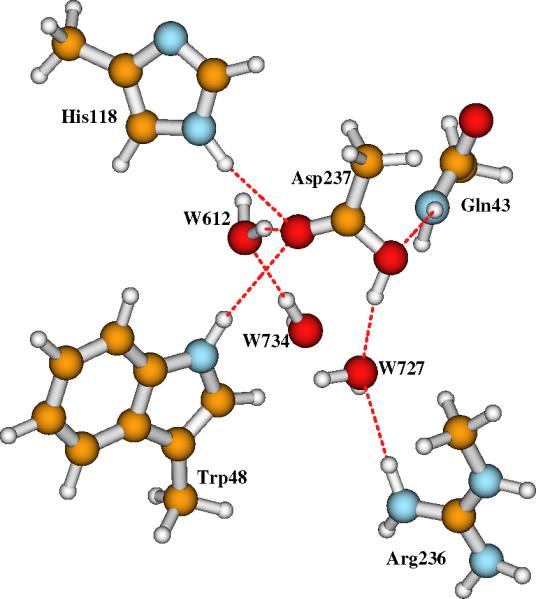
Since there are sulfate ions in the buffer of the ENDOR experiments, it is reasonable to propose that one or more sulfate ions interact with Arg236 and Lys42 on the surface of RNR-R2. In principle, any negatively charged group like a reductant, phosphate, and nitrate in solution can interact with the side chains of Arg236 and Lys42 in RNR-X. Next, taking sulfate as an example for the anion group, we will see how the interaction of sulfate and Arg236 will influence the pKa's of Asp237 and the bridging site O2. To mimic the solvation environment, we put six explicit water molecules around the sulfate. It is likely that the sulfate is in between Arg236 and Lys42, or two sulfates interact with Arg236 and Lys42 simultaneously. However, due to the large size of the quantum cluster and to be consistent with the models studied above, we add only one sulfate and 6 water molecules to Models I and II shown in Figure 5 and the corresponding Model-I-Asp237H and Model-II-Asp237H (Figure 8). The relative positions of Asp237, Water727, Arg236, and the sulfate plus water groups in the new models are shown in Figure 10. We will name these models as Model-I-SO42-, Model-II-SO42-, Model-I-Asp237H-SO42-, and Model-II-Asp237H-SO42-, respectively.
Figure 10.
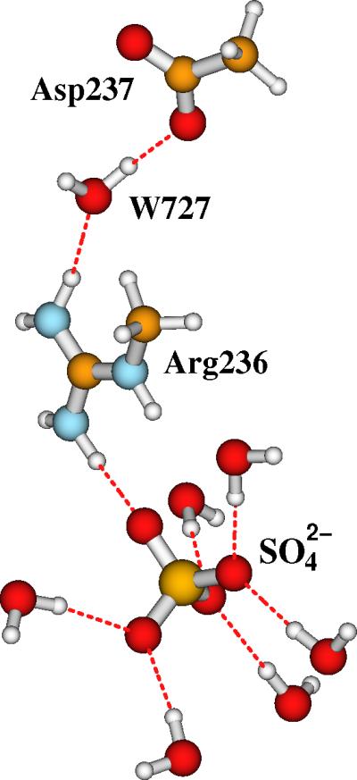
The relative positions of Arg236 and the sulfate plus six H-bonding water molecules in Model-I-SO42-, Model-II-SO42-, Model-I-Asp237H-SO42- and Model-II-Asp237H-SO42-. In Model-I-Asp237H-SO42- and Model-II-Asp237H-SO42-, the relative positions of the protonated Asp237, Water727, and Arg236 were shown in Figure 8.
To save the computer time, we optimized the four models in COSMO with only ε = 10. Then the DFT/PB-SCRF calculations were performed at the optimized geometries. The xyz Cartesian coordinates of these geometries are given in the Supporting Information. The calculated Mössbauer isomer shifts and quadrupole splittings, energies, and the pKa values of site O2 and Asp237 are shown in Table 5.
Table 5.
Calculated Isomer Shifts δ (mm s-1), Quadrupole Splittings (ΔEQ) (mm s-1), η, COSMO (with ε = 10) (EBS, -1147 eV) and DFT/PB-SCRF (Etotal, -1140 eV) Energies, and pKa's of Asp237 and Site O2 for Models I and II Interacting with SO42- and six water molecules and with/without Asp237 being Protonated.
| Model-I-SO42- |
Model-I-SO42--Asp237H |
Model-II-SO42- |
Model-II-SO42--Asp237H |
|||||
|---|---|---|---|---|---|---|---|---|
| COSMO | DFT/PB-SCRF | COSMO | DFT/PB-SCRF | COSMO | DFT/PB-SCRF | COSMO | DFT/PB-SCRF | |
| δ(Fe1) | 0.55 | 0.54 | 0.52 | 0.52 | ||||
| δ(Fe2) | 0.22 | 0.21 | 0.29 | 0.29 | ||||
| ΔEQ(Fe1) | -0.37 | 0.37 | 0.66 | 0.72 | ||||
| ΔEQ(Fe2) | -0.34 | -0.35 | -0.55 | -0.54 | ||||
| η(Fe1) | 0.75 | 0.72 | 0.66 | 0.64 | ||||
| η(Fe2) | 0.56 | 0.52 | 0.42 | 0.46 | ||||
| EBS or Etotal | -0.282 | -0.579 | -0.466 | -1.030 | -0.332 | -1.021 | -0.313 | -0.809 |
| pKa(O2{II → I + H+}) | 11.04 | 17.63 | 7.62 | 6.47 | ||||
| pKa(Asp237) | 12.81 | 17.31 | 9.40 | 6.15 | ||||
Adding the SO42- plus six water molecules in the quantum clusters of Model-I and Model-II do not change the Mössbauer properties of the diiron center. The single dielectric continuum model exhibits even more difficulty in describing such a complicated environment. The pKa's obtained from COSMO energies are different from the corresponding DFT/PB-SCRF results. We now focus on the energetic properties obtained from the DFT/PB-SCRF calculations which are given in bold. With sulfate interacting with Arg236, the protonated form of Asp237 is much more stabilized. The energy (-1141.030 eV) of Model-I-SO42--Asp237H is now the same as (actually a little lower than) the energy (-1141.021 eV) of Model-II-SO42-. When site O2 is not protonated, the DFT/PB-SCRF calculated pKa for Asp237 is 17.31 for the process {Model-I-SO42--Asp237H → Model-I-SO42- + H+}, which is essentially the same as the pKa of site O2 (17.63) in the process of {Model-II-SO42- → Model-I-SO42- + H+} when Asp237 is not protonated. These data show that Asp237 and site O2 have the same strong tendency to be protonated, when the alternative site is charged. On the other hand, if Asp237 is also protonated, the DFT/PB-SCRF calculated pKa for site O2 drops to only 6.47 (for the process {Model-II-SO42--Asp237H → Model-I-SO42--Asp237H + H+}). Similarly, if O2 is also protonated, the pKa of Asp237 also decreases sharply to 6.15 (for the process {Model-II-SO42--Asp237H → Model-II-SO42- + H+}). The pKa values predicted by the DFT/PB-SCRF calculations are more trustworthy than the simple COSMO calculations. But we are not saying that the DFT/PB-SCRF predicted pKa's are absolutely correct. Errors also exist in the zero-point energy differences, gas-phase proton energy, the solvation energy of a proton, the atomic charges in the protein field, and the embedded errors in general DFT and PB calculations. The large predicted pKa values 15.01 (in Table 2), 17.31 and 17.63 (in Table 5) show that our current DFT/PB-SCRF calculations may overestimate the pKa's, or these values may reflect the strong destabilization when both the diiron cluster and Asp237 are charged -1 anions in the presence of bound SO42-. In either event, the large pKa shifts from 17.31 to 6.15 and from 17.63 to 6.47 can tell us when the Asp237 and site O2 change from the protonated state to non-protonated state.
In summary, what we have learned from this section is that, when the anion group of SO42-+6H2O interact with Arg236, either Asp237 or the bridging site O2 has to be protonated. In another word, if Asp237 is protonated first, the O2 tends to be a bridging oxo; and if O2 is protonated as a bridging hydroxo, Asp237 then will stay in the charged form. Therefore, whether the diiron center in RNR-X stays in the di-μ-oxo (Model-I) or μ-oxo/μ-hydroxo (Model-II) form depends on whether an anion group like SO42- interacts with Arg236, and whether the Asp237 is protonated first or not. Since Model-I is the best active site structure to reproduce most of the properties obtained from the ENDOR experiments, we therefore propose that the RNR-X structure characterized by ENDOR experiments contains the Fe(III)(di-μ-oxo)Fe(IV) center with Asp237 protonated and an anion group interacting with the Arg236 (and possibly also with Lys42) side chain.
We have taken sulfate as the anion group in above calculations, since sulfates exist in the buffer of the ENDOR experiments. In living systems, the anion group can be phosphate or any other negatively charged group(s). Recall that before RNR-X is formed, a molecular oxygen (O2) binds to the Fe(II)-Fe(II) diiron center of R2red. After the O=O bond breaking, the diiron center should be similar to the intermediate Q of MMO which is in the Fe(IV)(di-μ-oxo)Fe(IV) state.68,69 In RNR, this is expected to be a highly transient state. Then an electron is transferred from Trp48 to one of the iron sites to make an Fe(III)(di-μ-oxo)Fe(IV) center with positive Trp48•+. There must be a reductant near the Trp48•+ to transfer an electron back to Trp48•+.94 The reductants are generally negatively charged.95,96 It is likely that the reductant will bind to the R2 surface through interaction with the side chains of Lys42 and Arg236 which are close to Trp48. Since Asp237 is close to the R2 surface and is surrounded by several water molecules, it is easier for Asp237 than site O2 to be protonated first after the Trp48•+ is 1e- reduced by the reductant. We emphasize that while the Trp48•+ is present, both the nearby Asp237- and the Fe(III)(di-μ-oxo)Fe(IV) anion are electrostatically stabilized. When Asp237 is protonated, the Fe(III)Fe(IV) center in RNR-X then favors the di-μ-oxo bridge (Model-I) rather than the one-μ-oxo/one-μ-hydroxo bridges (Model-II).
5. Conclusions
Two protonation states of RNR intermediate X models have been studied here. One is the Fe(III)Fe(IV) center with two bridging μ-oxo's. The other has one-μ-oxo and one-μ-hydroxo bridges. The latter is energetically more stable under a number of reasonable physical conditions. However, the former is more consistent with ENDOR experiments. Calculations show that if an anion group interacts with the side chain of Arg236 at the protein surface of RNR-R2, the carboxylate group of Asp237 favors the neutral protonated form particularly when the diiron cluster is initially an anion (-1 counting first shell ligands). In such situation, the diiron center of RNR-X remains an anion with two μ-oxo bridges. The protonation state forms a kinetic trap. We have used sulfate as the anion group in our current study, since sulfates exist in the buffer of ENDOR and MCD experiments. In real biological environments, this anion group can be a reductant like a ferredoxin, phosphate, or negatively charged groups in RNR-R1. Ascorbate or excess Fe2+ are non-physiological reductants in many spectroscopic and kinetics experiments. More experimental and theoretical studies are needed to further investigate how R1 and R2 bind,97,98 how the reductant interacts with R2, and how anion groups interact with Arg236 and Lys42 on the surface of R2. Depending on how long the anion groups stay in touch with Arg236 and Lys42, the active site of RNR-X can also be a mixture of Model-I and Model-II.
How the dielectric constant used in the COSMO continuum solvent model influences the central geometry, Mössbauer, and pKa properties is also studied here. For current large quantum cluster models which include the main polar groups up to the 4th coordination shells of the residues from the iron centers, changing of the dielectric constant in COSMO in the range of [4, 20] changes the main Fe-ligand distances, Mössbauer, and hyperfine properties very little. However, the relative energies and thus the pKa's predicted by the COSMO calculations are highly dependent on the dielectric constants. Choosing the dielectric constant to best predict the pKa's is system and site dependent. Caution needs to be taken when comparing relative energies and pKa's of metalloprotein active site models embedded in a simple continuum dielectric solvent environment.
Returning to the experimental dilemma, one significant difference between the ENDOR17 and the MCD19 experiments is the presence of high glycerol concentration in the MCD buffer solution. It may be that these different buffers lead to somewhat different R2 protein structures and aqueous solvent (or glycerol) access to the active site cluster. We have proposed that Asp237- is protonated first after 1e- reduction of Trp48•+, but there may be alternative protonation pathways into the Fe dimer cluster in the context of the MCD experiments. It should be feasible to perform EXAFS experiments and analysis based on sample preparations both from ENDOR and MCD. As shown in Table 1, there should be significant differences in Fe-Fe and Fe-O(H) distances depending on the protonation state of the oxo (hydroxo) bridges.
Supporting Information
Acknowledgment
We thank NIH for financial support (GM43278 to L.N.). The support of computer resources of the Scripps Research Institute is also gratefully acknowledged.
Footnotes
Supporting Information The Cartesian coordinates of Model-I and Model-II with three explicit H-bonding water molecules around site O2, and the coordinates of Model-I-SO42-, Model-II-SO42-, Model-IAsp237H-SO42- and Model-II-Asp237H-SO42- are given as supporting information. These structures were geometry optimized in COSMO solvation model with ε = 10 using DFT OPBE potential.
References
- 1.Wallar BJ, Lipscomb JD. Chem. Rev. 1996;96:2625–2658. doi: 10.1021/cr9500489. [DOI] [PubMed] [Google Scholar]
- 2.Sjöberg BM. Struct. Bond. 1997;88:139–173. [Google Scholar]
- 3.Bollinger JM, Jr., Edmondson DE, Huynh BH, Filley J, Norton JR, Stubbe J. Science. 1991;253:292–298. doi: 10.1126/science.1650033. [DOI] [PubMed] [Google Scholar]
- 4.Bollinger JM, Jr., Stubbe J, Huynh BH, Edmondson DE. J. Am. Chem. Soc. 1991;113:6289–6291. [Google Scholar]
- 5.Ravi N, Bollinger JM, Jr., Huynh BH, Edmondson DE, Stubbe J. J. Am. Chem. Soc. 1994;116:8007–8014. [Google Scholar]
- 6.Ravi N, Bominaar EL. Inorg. Chem. 1995;34:1040–1043. [Google Scholar]
- 7.Bollinger JM, Jr., Tong WH, Ravi N, Huynh BH, Edmondson DE, Stubbe J. In: Methods in Enzymology. Editon edn. Klinman JP, editor. Academic Press; New York: 1995. p. 258. [DOI] [PubMed] [Google Scholar]
- 8.Sturgeon BE, Burdi D, Chen SX, Huynh BH, Edmondson DE, Stubbe J, Hoffman BM. J. Am. Chem. Soc. 1996;118:7551–7557. [Google Scholar]
- 9.Nordlund P, Eklund H. J. Mol. Biol. 1993;232:123–164. doi: 10.1006/jmbi.1993.1374. [DOI] [PubMed] [Google Scholar]
- 10.Logan DT, Su XD, Aberg A, Regnstrom K, Hajdu J, Eklund H, Nordlund P. Structure. 1996;4:1053–1064. doi: 10.1016/s0969-2126(96)00112-8. [DOI] [PubMed] [Google Scholar]
- 11.Bollinger JM, Tong WH, Ravi N, Huynh BH, Edmondson DE, Stubbe J. J. Am. Chem. Soc. 1994;116:8015–8023. [Google Scholar]
- 12.Bollinger JM, Tong WH, Ravi N, Huynh BH, Edmondson DE, Stubbe J. J. Am. Chem. Soc. 1994;116:8024–8032. [Google Scholar]
- 13.Burdi D, Sturgeon BE, Tong WH, Stubbe JA, Hoffman BM. J. Am. Chem. Soc. 1996;118:281–282. [Google Scholar]
- 14.Veselov A, Scholes CP. Inorg. Chem. 1996;35:3702–3705. [Google Scholar]
- 15.Willems JP, Lee HI, Burdi D, Doan PE, Stubbe J, Hoffman BM. J. Am. Chem. Soc. 1997;119:9816–9824. [Google Scholar]
- 16.Riggs-Gelasco PJ, Shu LJ, Chen SX, Burdi D, Huynh BH, Que L, Stubbe J. J. Am. Chem. Soc. 1998;120:849–860. [Google Scholar]
- 17.Burdi D, Willems J-P, Riggs-Gelasco P, Antholine WE, Stubbe J, Hoffman BM. J. Am. Chem. Soc. 1998;120:12910–12919. [Google Scholar]
- 18.Shanmugam M, Doan PE, Lees NS, Stubbe J, Hoffman BM. J. Am. Chem. Soc. 2009;131:3370–3376. doi: 10.1021/ja809223s. [DOI] [PMC free article] [PubMed] [Google Scholar]
- 19.Mitić N, Saleh L, Schenk G, Bollinger JMJ, Solomon EI. J. Am. Chem. Soc. 2003;125:11200–11201. doi: 10.1021/ja036556e. [DOI] [PubMed] [Google Scholar]
- 20.Baldwin J, Krebs C, Ley BA, Edmondson DE, Huynh BH, Bollinger JH. J. Am. Chem. Soc. 2000;122:12195–12206. [Google Scholar]
- 21.Krebs C, Chen SX, Baldwin J, Ley BA, Patel U, Edmondson DE, Huynh BH, Bollinger JM. J. Am. Chem. Soc. 2000;122:12207–12219. [Google Scholar]
- 22.Siegbahn PEM. Inorg. Chem. 1999;38:2880–2889. doi: 10.1021/ic981332w. [DOI] [PubMed] [Google Scholar]
- 23.Siegbahn EM. Quarterly Reviews of Biophysics. 2003;36:91–145. doi: 10.1017/s0033583502003827. [DOI] [PubMed] [Google Scholar]
- 24.Han W-G, Lovell T, Liu T, Noodleman L. Inorg. Chem. 2003;42:2751–2758. doi: 10.1021/ic020465l. [DOI] [PubMed] [Google Scholar]
- 25.Han W-G, Lovell T, Liu T, Noodleman L. Inorg. Chem. 2004;43:613–621. doi: 10.1021/ic0206443. [DOI] [PubMed] [Google Scholar]
- 26.Han W-G, Liu T, Lovell T, Noodleman L. J. Am. Chem. Soc. 2005;127:15778–15790. doi: 10.1021/ja050904q. [DOI] [PubMed] [Google Scholar]
- 27.Han WG, Liu TQ, Lovell T, Noodleman L. Inorg. Chem. 2006;45:8533–8542. doi: 10.1021/ic060566+. [DOI] [PubMed] [Google Scholar]
- 28.Han W-G, Liu T, Lovell T, Noodleman L. J. Inorg. Biochem. 2006;100:771–779. doi: 10.1016/j.jinorgbio.2006.01.032. [DOI] [PubMed] [Google Scholar]
- 29.Younker JM, Krest CM, Jiang W, Krebs C, Bollinger JM, Green MT. J. Am. Chem. Soc. 2008;130:15022–15027. doi: 10.1021/ja804365e. [DOI] [PMC free article] [PubMed] [Google Scholar]
- 30.Jiang W, Yun D, Saleh L, Bollinger JM, Krebs C. Biochemistry. 2008;47:13736–13744. doi: 10.1021/bi8017625. [DOI] [PMC free article] [PubMed] [Google Scholar]
- 31.Jiang W, Saleh L, Barr EW, Xie JJ, Gardner MM, Krebs C, Bollinger JM. Biochemistry. 2008;47:8477–8484. doi: 10.1021/bi800881m. [DOI] [PMC free article] [PubMed] [Google Scholar]
- 32.Miti N, Clay MD, Saleh L, Bollinger JMJ, Solomon EI. J. Am. Chem. Soc. 2007;129:9049–9065. doi: 10.1021/ja070909i. [DOI] [PMC free article] [PubMed] [Google Scholar]
- 33.Klamt A, Schüürmann G. J. Chem. Soc. Perkin Trans. II. 1993:799–805. [Google Scholar]
- 34.Klamt A. J. Phys. Chem. 1995;99:2224–2235. [Google Scholar]
- 35.Klamt A, Jonas V. J. Chem. Phys. 1996;105:9972–9981. [Google Scholar]
- 36.Pye CC, Ziegler T. Theor. Chem. Acc. 1999;101:396–408. [Google Scholar]
- 37.Harvey SC, Hoekstra P. J. Phys. Chem. 1972;76:2987–2994. doi: 10.1021/j100665a011. [DOI] [PubMed] [Google Scholar]
- 38.Bone S, Pethig R. J. Mol. Biol. 1982;157:571–575. doi: 10.1016/0022-2836(82)90477-6. [DOI] [PubMed] [Google Scholar]
- 39.Bone S, Pethig R. J. Mol. Biol. 1985;181:323–326. doi: 10.1016/0022-2836(85)90096-8. [DOI] [PubMed] [Google Scholar]
- 40.Dwyer JJ, Gittis AG, Karp DA, Lattman EE, Spencer DS, Stites WE, Garcia-Moreno B. Biophys. J. 2000;79:1610–1620. doi: 10.1016/S0006-3495(00)76411-3. [DOI] [PMC free article] [PubMed] [Google Scholar]
- 41.Han W-G, Noodleman L. Theor. Chem. Accounts. 2009 in press. [Google Scholar]
- 42.Gregg EC. Handbook of Chemistry and Physics. Editon edn. Chemical Rubber Company; Cleveland, OH: 1976. pp. E55–E60. [Google Scholar]
- 43.Sham YY, Muegge I, Warshel A. Biophys. J. 1998;74:1744–1753. doi: 10.1016/S0006-3495(98)77885-3. [DOI] [PMC free article] [PubMed] [Google Scholar]
- 44.Bashford D, Karplus M. Biochemistry. 1990;29:10219–10225. doi: 10.1021/bi00496a010. [DOI] [PubMed] [Google Scholar]
- 45.Fitch CA, Karp DA, Lee KK, Stites WE, Lattman EE, Garcia-Moreno B. Biophys. J. 2002;82:3289–3304. doi: 10.1016/s0006-3495(02)75670-1. [DOI] [PMC free article] [PubMed] [Google Scholar]
- 46.Antosiewicz J, McCammon JA, Gilson MK. Biochemistry. 1996;35:7819–7833. doi: 10.1021/bi9601565. [DOI] [PubMed] [Google Scholar]
- 47.Simonson T, Brooks CL. J. Am. Chem. Soc. 1996;118:8452–8458. [Google Scholar]
- 48.Karp DA, Gittis AG, Stahley MR, Fitch CA, Stites WE, Garcia-Moreno B. Biophys. J. 2007;92:2041–2053. doi: 10.1529/biophysj.106.090266. [DOI] [PMC free article] [PubMed] [Google Scholar]
- 49.Harms MJ, Schlessman JL, Chimenti MS, Sue GR, Damjanovic A, Garcia-Moreno B. Protein Science. 2008;17:833–845. doi: 10.1110/ps.073397708. [DOI] [PMC free article] [PubMed] [Google Scholar]
- 50.Chen JL, Noodleman L, Case DA, Bashford D. J. Phys. Chem. 1994;98:11059–11068. [Google Scholar]
- 51.Bashford D. In: Scientific Computing in Object-Oriented Parallel Environments (Lecture Notes in Computer Science) Editon edn. Ishikawa Y, Oldehoeft RR, Reynders JVW, Tholburn M, editors. vol. 1343. Springer; Berlin: 1997. pp. 233–240. [Google Scholar]
- 52.Li J, Nelson MR, Peng CY, Bashford D, Noodleman L. J. Phys. Chem. A. 1998;102:6311–6324. [Google Scholar]
- 53.Liu T, Han W-G, Himo F, Ullmann GM, Bashford D, Toutchkine A, Hahn KM, Noodleman L. J. Phys. Chem. A. 2004;108:3545–3555. [Google Scholar]
- 54.Han W-G, Liu T, Himo F, Toutchkine A, Bashford D, Hahn KM, Noodleman L. ChemPhysChem. 2003;4:1084–1094. doi: 10.1002/cphc.200300801. [DOI] [PubMed] [Google Scholar]
- 55.Toutchkine A, Han W-G, Ullmann M, Liu TQ, Bashford D, Noodleman L, Hahn KM. J. Phys. Chem. A. 2007;111:10849–10860. doi: 10.1021/jp073197r. [DOI] [PMC free article] [PubMed] [Google Scholar]
- 56.Sitkoff D, Sharp KA, Honig B. J. Phys. Chem. 1994;98:1978–1988. [Google Scholar]
- 57.Han W-G, Tajkhorshid E, Suhai S. J. Biomol. Struct. Dyn. 1999;16:1019–1032. doi: 10.1080/07391102.1999.10508311. [DOI] [PubMed] [Google Scholar]
- 58.ADF2006.01, SCM. Editon edn. Theoretical Chemistry, Vrije Universiteit; Amsterdam, The Netherlands: http://www.scm.com. [Google Scholar]
- 59.te Velde G, Bickelhaupt FM, Baerends EJ, Guerra CF, Van Gisbergen SJA, Snijders JG, Ziegler T. J. Comput. Chem. 2001;22:931–967. [Google Scholar]
- 60.Guerra CF, Snijders JG, te Velde G, Baerends EJ. Theor. Chem. Acc. 1998;99:391–403. [Google Scholar]
- 61.Vosko SH, Wilk L, Nusair M. Can. J. Phys. 1980;58:1200–1211. [Google Scholar]
- 62.Perdew JP, Burke K, Ernzerhof M. Phys. Rev. Lett. 1996;77:3865–3868. doi: 10.1103/PhysRevLett.77.3865. [DOI] [PubMed] [Google Scholar]
- 63.Perdew JP, Burke K, Ernzerhof M. Phys. Rev. Lett. 1997;78:1396–1396. doi: 10.1103/PhysRevLett.77.3865. [DOI] [PubMed] [Google Scholar]
- 64.Handy NC, Cohen AJ. Molec. Phys. 2001;99:403–412. [Google Scholar]
- 65.Swart M, Groenhof AR, Ehlers AW, Lammertsma K. J. Phy. Chem. A. 2004;108:5479–5483. [Google Scholar]
- 66.Swart M, Ehlers AW, Lammertsma K. Molec. Phys. 2004;102:2467–2474. [Google Scholar]
- 67.Swart M. J. Chem. Theory Comput. 2008;4:2057–2066. doi: 10.1021/ct800277a. [DOI] [PubMed] [Google Scholar]
- 68.Han WG, Noodleman L. Inorg. Chim. Acta. 2008;361:973–986. doi: 10.1016/j.ica.2007.06.007. [DOI] [PMC free article] [PubMed] [Google Scholar]
- 69.Han W-G, Noodleman L. Inorg. Chem. 2008;47:2975–2986. doi: 10.1021/ic701194b. [DOI] [PubMed] [Google Scholar]
- 70.Perdew JP, Chevary JA, Vosko SH, Jackson KA, Pederson MR, Singh DJ, Fiolhais C. Phys. Rev. B. 1992;46:6671–6687. doi: 10.1103/physrevb.46.6671. [DOI] [PubMed] [Google Scholar]
- 71.Noodleman L. J. Chem. Phys. 1981;74:5737–5743. [Google Scholar]
- 72.Noodleman L, Case DA. Adv. Inorg. Chem. 1992;38:423–470. [Google Scholar]
- 73.Noodleman L, Lovell T, Han W-G, Liu T, Torres RA, Himo F. In: Comprehensive Coordination Chemistry II, From Biology to Nanotechnology. Editon edn. Lever AB, editor. vol. 2. Elsevier Ltd; 2003. pp. 491–510. [Google Scholar]
- 74.Han W-G, Liu TQ, Lovell T, Noodleman L. J. Comput. Chem. 2006;27:1292–1306. doi: 10.1002/jcc.20402. [DOI] [PubMed] [Google Scholar]
- 75.Martinez-Pinedo G, Schwerdtfeger P, Caurier E, Langanke K, Nazarewicz W, Sohnel T. Physical Review Letters. 2001;87:062701, 062701–062704. doi: 10.1103/PhysRevLett.87.062701. [DOI] [PubMed] [Google Scholar]
- 76.Noodleman L, Chen JL, Case DA, Giori C, Rius G, Mouesca JM, Lamotte B. In: Nuclear Magnetic Resonance of Paramagnetic Macromolecules. Editon edn. La Mar GN, editor. Kluwer Academic Publishers; Netherland: 1995. pp. 339–367. [Google Scholar]
- 77.Sinnecker S, Neese F, Noodleman L, Lubitz W. J. Am. Chem. Soc. 2004;126:2613–2622. doi: 10.1021/ja0390202. [DOI] [PubMed] [Google Scholar]
- 78.Breneman CM, Wiberg KB. J. Comput. Chem. 1990;11:361–373. [Google Scholar]
- 79.Mouesca JM, Chen JL, Noodleman L, Bashford D, Case DA. J. Am. Chem. Soc. 1994;116:11898–11914. [Google Scholar]
- 80.Bashford D. Curr. Opin. Struct. Biol. 1991;1:175–184. [Google Scholar]
- 81.Bashford D, Gerwert K. J. Mol. Biol. 1992;224:473–486. doi: 10.1016/0022-2836(92)91009-e. [DOI] [PubMed] [Google Scholar]
- 82.Lim C, Bashford D, Karplus M. J. Phys. Chem. 1991;95:5610–5620. [Google Scholar]
- 83.Bashford D, Case DA, Dalvit C, Tennant L, Wright PE. Biochemistry. 1993;32:8045–8056. doi: 10.1021/bi00082a027. [DOI] [PubMed] [Google Scholar]
- 84.Tissandier MD, Cowen KA, Feng WY, Gundlach E, Cohen MH, Earhart AD, Coe JV, Tuttle TR. J. Phys. Chem. A. 1998;102:7787–7794. [Google Scholar]
- 85.Lewis A, Bumpus JA, Truhlar DG, Cramer CJ. J. Chem. Edu. 2004;81:596–604. [Google Scholar]
- 86.Lewis A, Bumpus JA, Truhlar DG, Cramer CJ. J. Chem. Edu. 2007;84:934. [Google Scholar]
- 87.Tawa GJ, Topol IA, Burt SK, Caldwell RA, Rashin AA. J. Chem. Phys. 1998;109:4852–4863. [Google Scholar]
- 88.Baes CJ, Mesmer RE. The hydrolysis of Cations. Krieger; Malabar, India: 1986. [Google Scholar]
- 89.Flynn CM. Chem. Rev. 1984;84:31–41. [Google Scholar]
- 90.Elango N, Radhakrishnan R, Froland WA, Wallar BJ, Earhart CA, Lipscomb JD, Ohlendorf DH. Protein Sci. 1997;6:556–568. doi: 10.1002/pro.5560060305. [DOI] [PMC free article] [PubMed] [Google Scholar]
- 91.Jungwirth P, Winter B. Annu. Rev. Phys. Chem. 2008;59:343–366. doi: 10.1146/annurev.physchem.59.032607.093749. [DOI] [PubMed] [Google Scholar]
- 92.Vrbka L, Jungwirth P, Bauduin P, Touraud D, Kunz W. J. Phys. Chem. B. 2006;110:7036–7043. doi: 10.1021/jp0567624. [DOI] [PubMed] [Google Scholar]
- 93.Chakrabarti P. J. Mol. Biol. 1993;234:463–482. doi: 10.1006/jmbi.1993.1599. [DOI] [PubMed] [Google Scholar]
- 94.Hristova D, Wu CH, Jiang W, Krebs C, Stubbe J. Biochemistry. 2008;47:3989–3999. doi: 10.1021/bi702408k. [DOI] [PMC free article] [PubMed] [Google Scholar]
- 95.Wu CH, Jiang W, Krebs C, Stubbe JA. Biochemistry. 2007;46:11577–11588. doi: 10.1021/bi7012454. [DOI] [PubMed] [Google Scholar]
- 96.Cotruvo JA, Stubbe J. PNAS. 2008;105:14383–14388. doi: 10.1073/pnas.0807348105. [DOI] [PMC free article] [PubMed] [Google Scholar]
- 97.Stubbe J, Nocera DG, Yee CS, Chang MCY. Chem. Rev. 2003;103:2167–2201. doi: 10.1021/cr020421u. [DOI] [PubMed] [Google Scholar]
- 98.Sjöberg BM. Structure. 1994;2:793–796. doi: 10.1016/s0969-2126(94)00080-8. [DOI] [PubMed] [Google Scholar]
Associated Data
This section collects any data citations, data availability statements, or supplementary materials included in this article.