Sensorimotor rhythm-based brain-computer interface (BCI): model order selection for autoregressive spectral analysis

Abstract

People can learn to control EEG features consisting of sensorimotor rhythm amplitudes and can use this control to move a cursor in one or two dimensions to a target on a screen. Cursor movement depends on the estimate of the amplitudes of sensorimotor rhythms. Autoregressive models are often used to provide these estimates. The order of the autoregressive model has varied widely among studies. Through analyses of both simulated and actual EEG data, the present study examines the effects of model order on sensorimotor rhythm measurements and BCI performance. The results show that resolution of lower frequency signals requires higher model orders; and that this requirement reflects the temporal span of the model coefficients. This is true for both simulated EEG data and actual EEG data during brain-computer interface (BCI) operation. Increasing model order and decimating the signal were similarly effective in increasing spectral resolution. Furthermore, for BCI control of two-dimensional cursor movement, higher model orders produced better performance in each dimension and greater independence between horizontal and vertical movements. In sum, these results show that autoregressive model order selection is an important determinant of BCI performance and should be based on criteria that reflect system performance.

1. Introduction

Many people with severe motor disabilities require alternative methods for communication and control. Numerous studies over the past two decades indicate that scalp-recorded EEG activity can be the basis for non-muscular communication and control systems, commonly called brain-computer interfaces (BCIs) (Birbaumer et al, 1999; Farwell and Donchin, 1988; Pfurtscheller et al, 1993; Wolpaw et al, 1991). EEG-based communication systems measure specific features of EEG activity and use the results as control signals. In some systems, these features are potentials evoked by stereotyped stimuli (Wolpaw et al, 2002). Other systems use EEG components in the frequency domain that are spontaneous in the sense that they are not dependent on specific sensory events (e.g., Wolpaw and McFarland, 1991 and 2004).

With the Wadsworth sensorimotor rhythm-based BCI system, users learn over a series of training sessions to use sensorimotor rhythm amplitudes in a mu (8–13 Hz) or beta (18–27 Hz) frequency band over left and/or right sensorimotor cortex to move a cursor on a video screen in one or two dimensions (see McFarland et al, 2006 for full system description). We use an autoregressive model to estimate these sensorimotor rhythm amplitudes. This autoregressive model can be expressed as:

$$Y_t={\displaystyle \sum _{i=1}^{i=p}{w}_{t-i}{Y}_{t-i}+e}$$ 1)

where Y_t is the predicted signal at time t, w is a vector of p coefficients, and e is the prediction error.

Autoregressive modeling requires selection of a data window length (i.e., duration) and a model order. Selection of these parameters has varied widely across different studies. For example, Schlogl et al (2005) used a model order of 3, Ince et al (2006) used an order of 6, and McFarland and Wolpaw (2005) used an order of 16. The data window length is the duration in time of the EEG segment used for each individual spectral estimate. This parameter has also varied considerably. For example, Fabiani et al (2004) used 200 msec while Kelley et al (2002) used 1500 msec. Studies that use adaptive algorithms to estimate autoregressive coefficients (e.g., Schlogl et al, 2005) can be regarded as employing an exponential data window. With Fourier-based spectral analysis, the length of the data window determines spectral resolution such that the resolution in Hz is equal to the reciprocal of this duration in seconds. With autoregressive spectral analysis, this relationship is not similarly straightforward (Marple, 1987). Some authors have asserted that autoregressive models provide infinite resolution (e.g. Florian and Pfurtscheller, 1995). In reality, autoregressive models can provide spectral estimates for segments of any duration. However, this does not mean that signals can be resolved with infinite precision.

The model order refers to the number of prior predictions used in the model, (i.e., p in 1). Authors have provided various rationales for their choice of model order. For example, Floran and Pfurtscheller (1995) noted that the choice of model order should be based on a consideration of both the signal complexity and the sampling rate. An objective method of selecting p is to minimize Akaike’s Information Criterion (AIC) (Akaike, 1974)), which is a weighted combination of prediction error and model complexity. However there is considerable disagreement about the optimal tradeoff between error and complexity (for a review see Stoica and Selen, 2004).

The typical BCI protocol that uses parametric spectral methods can have at least two types of prediction errors. The first of these is the error in predicting the EEG waveform and is the measure used by AIC. We will refer to this as the signal prediction error. The second of these is the error in predicting the target position and can be expressed as 1−r² (Sheikh et al, 2003). We will refer to this as the target prediction error. One rational for keeping the model order as low as possible is that simple models generalize better, since fewer parameters result in fewer estimation errors. However, generalization of the model is not a consideration in the typical BCI application, since new parameters are estimated for each data window. An additional consideration is that higher model orders may lead to the identification of false spectral peaks (Marple, 1987).

We have recently compared model selection based on minimizing signal prediction error (i.e., use of AIC) with that based on minimizing target prediction error (i.e., use of r²). The use of AIC resulted in much lower model order selections than selection based on optimizing r² ( Krusienski et al, 2006). We argued that r² optimizes BCI-based communication and control, and thus is the more desirable method for BCI purposes. Bufalari et al (2006) have also shown that higher model orders are needed to optimize r² values with BCI data.

While model order selection based on empirically optimizing r² is a useful approach, we sought to learn why higher order models work better. In the present investigation, we examined the effects of model order on analyses of simple synthetic signals with known spectral content. The results show that larger model orders are better suited for autoregressive analyses of low frequency signals obscured by noise. We go on to show that this principle applies to actual BCI data.

2. Methods

Simulated data

Simulated data were constructed by adding one or two sine waves to the output of the random number generator in Borland Builder 6. Both sine waves and the noise were of equal variance. The data were stored in ASCII files and subsequently analyzed with the Berg algorithm (Press et al, 1988) implemented with custom software.

Users

For analyses of one-dimensional cursor control, the BCI users were 7 adults (5 men, and 2 woman, ages 20–39). Five had no disabilities, while two had spinal cord injuries (at C6 and T7) and were confined to wheelchairs. For analyses of two-dimensional cursor control, the users were 8 adults, 4 of whom had contributed data to the 1D analysis. All gave informed consent for the study, which had been reviewed and approved by the New York State Department of Health Institutional Review Board. After an initial evaluation defined the frequencies and scalp locations of each person’s spontaneous mu and beta rhythm (i.e., sensorimotor rhythm) activity, he or she learned EEG-based cursor control over several months (2–3 sessions/week). The standard online protocol, which has been described in previous publications (McFarland et al, 1997; Schalk et al, 2004; Wolpaw and McFarland, 2004), is summarized here.

Standard Online Protocol

The user sat in a reclining chair facing a 51-centimeter video screen three m away, and was asked to remain motionless during performance. Scalp electrodes recorded 64 channels of EEG (Sharbrough et al, 1991), each referenced to an electrode on the right ear (amplification 20,000; bandpass 0.1–60 Hz; sampling rate 160 Hz).

A daily session had 8 three-min runs separated by one-min breaks, and each run had 20–30 trials. Each trial consisted of a one-sec period from target appearance to the beginning of cursor movement, a two-sec period of cursor movement, a 1.5-sec post-movement reward period, and a one-sec inter-trial interval. Users participated in 2–3 sessions/week at a rate of one every 2–3 days.

To control vertical cursor movement, one EEG channel over left sensorimotor cortex (i.e., electrode locations C3 or CP3) and/or one channel over right sensorimotor cortex (i.e., C4 or CP4) were derived from the digitized data according to a Laplacian transform (McFarland et al, 1997). Every 50 msec, the most recent 400-msec segment from each channel was analyzed by a 16^th-order autoregressive model using the Berg algorithm (Marple, 1987) to determine the amplitude (i.e., square root of power) in a 3-Hz-wide mu or beta frequency band, and the amplitudes of the one or two channels were used in a linear equation that specified a cursor movement as described above. Thus, cursor movement occurred 20 times per sec. For two-dimensional control, additional channels or frequencies from sensorimotor cortex were used to control horizontal movement (see Wolpaw and McFarland, 2004 for details). Complete EEG and cursor movement data were stored for later offline analyses.

Stepwise Regression Analysis

In the standard online protocol, each user employed one or two mu or beta rhythm amplitudes over right or left sensorimotor cortex to control each dimension of cursor movement. BCI feature selection and translation was accomplished by stepwise regression. This was done separately for online training and for both model order conditions of the offline data analyses. To predict the online performance that would be achieved by controlling cursor movement with weighted combinations of mu and beta rhythm amplitudes from right and left sides, we calculated, in offline analyses of the data from each of the users, the correlations with target location of each amplitude (i.e., left mu, left beta, right mu, right beta) singly and in weighted combinations using the multiple regression procedure from SAS (SAS Institute Inc). Parameter estimates were determined using least-squares criteria and the normal equations:

$$(\mathrm{X}’\mathrm{X})b=\mathrm{X}’\mathrm{Y}$$ 3)

where X is a m by n matrix formed from the n observations of m predictor variables (i.e., EEG amplitudes at specific frequencies and locations) and Y is the vector of n values (i.e., target positions) to be predicted. Solving for b yields:

$$b={(\mathrm{X}’\mathrm{X})}^{-1}\mathrm{X}’\mathrm{Y}$$ 4)

Correlation was expressed as r², the proportion of the total variance in target location that was accounted for by the model for the two-sec cursor movement period.

We used the stepwise option as a feature selection heuristic. Briefly, we used a combination of forward and backward stepwise regression steps. Starting with no initial terms, the most statistically significant predictor variable with a p-value < 0.01 was added. After each new entry, a backward regression step removed any variables with p-values > 0.01. This iterative process continued until no additional terms satisfied the entry/removal criteria.

3. Results

Simulations

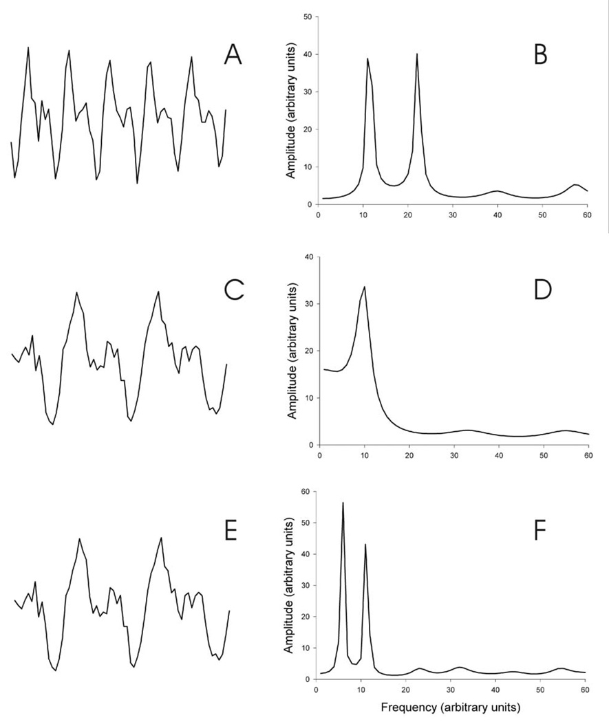
To explore the impact of model order, we systematically varied the period of two sine waves superimposed on noise of equal variance. The main finding, summarized in Figure 1, was that lower frequency stimuli require larger model orders. Figure 1a shows a simulated waveform composed of 64 samples (i.e., 64 points). The wave form was produced by adding two sine waves with periods of 12 and 6 samples, respectively, to noise. Figure 1b shows the corresponding autoregressive spectral analysis obtained using a model order of 8. The two sine waves appear as two narrow peaks. Figure 1c shows a 64-sample simulated waveform produced by adding two sine waves with periods of 12 and 24 samples, respectively, to the noise. Figure1d shows the corresponding autoregressive spectral analysis, again with a model order of 8. The two sine waves appear as a single broad peak. Figure 1e shows the same waveform as Figure 1c; and Figure 1f shows the corresponding autoregressive analysis with a model order of 16. Now, the two sine waves appear as two narrow peaks. Thus, the same 12-sample sine wave is resolved with model order 8 when it is combined with a higher frequency (i.e., 6-sample) sine wave, but not when it is combined with a lower frequency (i.e., 24-sample) sine wave. In the latter case, it is resolved with a model order of 16. Resolution of the 12-sample sine wave requires a larger model order when it is combined with a lower frequency signal than when it is combined with a higher frequency signal.

Figure 1.

Simulated waveforms and their corresponding spectra. A. B. Spectrum of A derived by an 8^th order autoregressive model. C. A 64-sample waveform comprised of two sine waves with periods of 12 and 24 samples and added noise. D. Spectrum of C derived by an 8^th order autoregressive model. E. Same as C. F. Spectrum of E derived by a 16^th order autoregressive model. Note that the same sine wave with a period of 6 samples was resolved by an 8^th order model when it was added to another sine wave with a period of 6 samples (B), but not when it was added to a sine wave with a period of 24 samples (D). Resolution of the latter two sine waves was achieved by a 16^th order model (F).

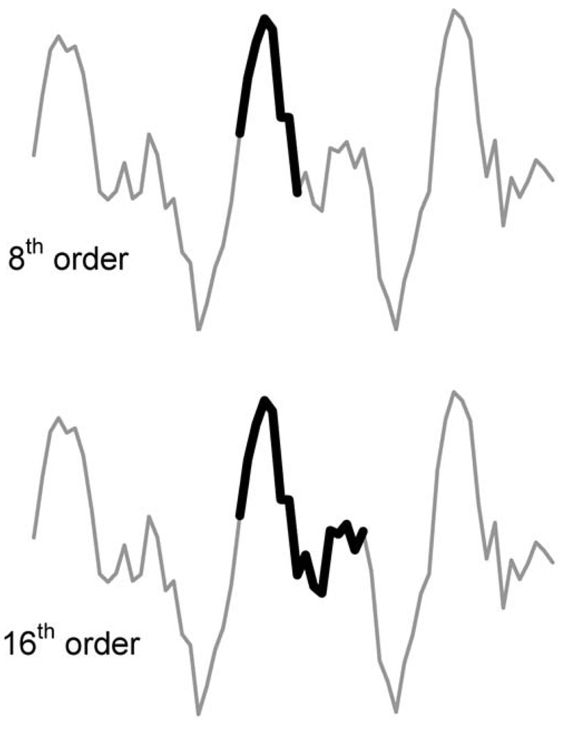
Figure 2 illustrates the difference between 8^th and 16^th order models in the length of the segment spanned by the AR model coefficients. It shows that the higher order model spans a greater portion of the signal. Figure 1 indicates that a longer time segment is needed when the signal contains components with longer periods (i.e., lower frequency components). Adequate spectral resolution requires that some minimal fraction of the lowest frequency component be spanned by the model coefficients. To the extent that the span of the model coefficient is the critical factor, it should be possible to produce spectra of similar resolution by either increasing the model order or decimating the signal.

Figure 2.

Samples spanned by 8^th and 16^th order models. Note how the span is twice as long with the 16^th order model as with the 8^th order model.

BCI data

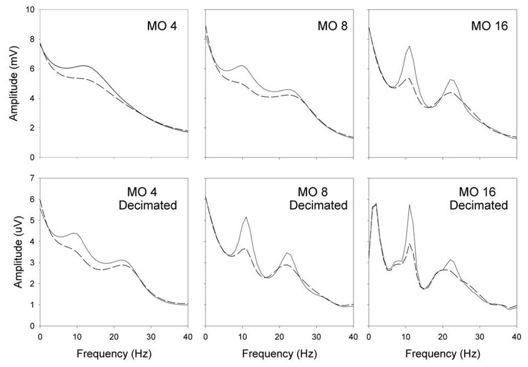
We went on to examine the impacts of different model orders and signal decimation in offline analyses of two-dimensional cursor control data from six BCI users. For each person’s data, spectral resolution increased with model order or with data decimation. Figure 3 shows a representative result. The sampling rate was 128 Hz. Model order 4 yields a single broad peak, model order 8 partially separates this broad peak into two distinct peaks, and model order 16 clearly resolves peaks at 11 and 22 Hz. With each model order, decimating the data by a factor of 2 had an effect very similar to doubling the model order. Thus, the spectra for model order 8 undecimated and model order 16 undecimated are very similar to those for model order 4 decimated and model order 8 decimated, respectively. These results illustrate the principle that the temporal span of the model coefficients is an important determinant of spectral resolution.

Figure 3.

Spectra from off-line analysis of data from one-dimensional cursor movement control. Solid lines represent top targets and dashed lines represent bottom targets. Spectra on the top are from data sampled at 128 Hz while those on the bottom are from the same data decimated by a factor of 2. From left to right are model orders of 4, 8, and 16. Note that decimating by a factor of 2 and increasing the model order by a factor of 2 have similar effects on spectral resolution.

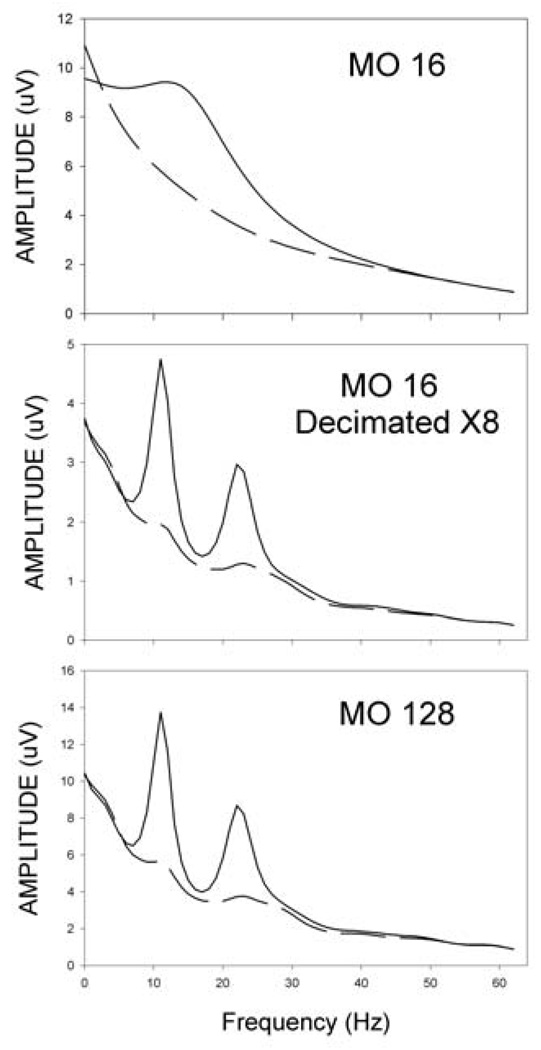
As a further test of this hypothesis we collected data with a sampling rate of 1280 Hz from two people controlling two-dimensional cursor movement. The higher sampling rate allowed exploration of a much greater range of model orders and decimation factors (i.e., 8x rather than only 2x). The analog filters were left at 0.1–60 Hz to limit the bandwidth of the signal. Figure 4 shows the results from one of these individuals. With this person’s data, a 16^th order model produces a single broad spectral peak. Decimating the data by a factor of 8 or increasing the model order by a factor of 8 resolves this single broad peak into two peaks of 11 and 22 Hz, respectively. Thus, a 16^th order model is adequate at an effective sampling frequency of 160 Hz but grossly inadequate at a sampling frequency of 1280 Hz. The length of the segment spanned by the adequate model orders is 100 msec for both the 16^th order model at 160 Hz and the 128^th order model at 1280 Hz. This example clearly demonstrates the impact of model order span.

Figure 4.

Spectra from offline analysis of data from one dimensional cursor movement control. Solid line represents top targets and dashed line represents bottom targets. The top plot shows spectra from data sampled at 1280 Hz and derived by a 16^th order autoregressive model. The middle graph shows the same data decimated by a factor of 8 and derived by a 16^th order model. The bottom graph shows the spectra of the data sampled at 1280 Hz and derived by a 128^th order model. Note that decimating the data by a factor of 8 has essentially the same effect as increasing the model order by a factor of 8.

We previously showed that higher model orders lead to better prediction of target position for a one-dimensional cursor movement protocol (Krusienski et al, 2006; McFarland et al, 2006). To extend this finding, we examined the impact of model order in an offline analysis of two-dimensional cursor movement (Wolpaw and McFarland, 2004). This extension allows evaluation of both the target prediction accuracy and the independence of the horizontal and vertical control signals.

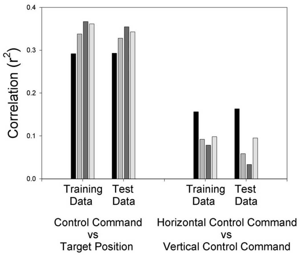
Data from each of 8 individuals were analyzed with 4^th, 8^th, 16^th, and 32^nd order autoregressive models, using the spectral bands and weights determined by stepwise regression of five 3-Hz wide spectral bands over left and right sensorimotor cortices (e.g., locations C3 and C4 or CP3 and CP4, depending on the individual). Regressions were done separately for each model order and target dimension on data from three sessions from each person. The results were then generalized to data from 3 more sessions from that person. Figure 5 shows the results. Increasing the model order gave better predictions of target position in each dimension and also gave greater independence of the predictions for the two dimensions. For the target prediction metric, a factorial analysis of variance including dimension, model order, and training (i.e., first 3 sessions) vs test (i.e., next 3 sessions) phase indicated that only the effects of model order were significant (p < 0.0007). For the independence metric, a factorial analysis of variance including model order and training vs test phase indicated that the effect of model order was just short of significance (p < 0.07). Thus higher model order gave both better target prediction in each dimensions and greater independence between the control signals for the two dimensions.

Figure 5.

Average r² values for data from 8 subjects controlling two-dimensional cursor movement. Multidimensional regression models were derived from 3 sessions of data (i.e., training sessions)and generalized to 3 more sessions (i.e., test data). Black bars represent a 4^th order model, light bars represent an 8^th order model, dark grey bars represent a 16^th order model, and the lightest bars represent a 32^nd order model. Note that correlation with the position of the target is higher (i.e., r² averaged over both dimensions) while the correlation between the horizontal and vertical control commands is lower for the higher model orders. Thus, the higher model orders provide better cursor control.

4. Discussion

In the present study, analyses of both simulated and actual EEG data show that the time interval spanned by the autoregressive coefficients is an important determinant of spectral resolution. This effect may be somewhat analogous to the relationship between resolution and window length with classic Fourier analysis. The study also demonstrates that, for two-dimensional BCI movement control, spectral resolution influences both prediction accuracy in each dimension and independence between the control signals for the two dimensions. For such multidimensional control, this independence may be as important for performance as is the accuracy of prediction in each dimension.

The traditional approach to model order selection views the problem in terms of minimizing both prediction error and model complexity (e.g., Stoica and Selen, 2004). This is the basis for model order selection by algorithms such as Akaike’s information criterion. Selection of the relative weight to be given to these two competing factors is arbitrary, since there is no objective way of assessing their relative importance. In addition, the two are not quantified in terms of the same units of measurement. More important however, is the fact that model complexity is not directly related to BCI performance-related criteria such as accuracy (i.e., the proportion of trials that hit the target) Thus, target prediction error should be the primary guide to model order selection (Krusienski et al, 2006).

Although it has been stated that autoregressive spectra have infinite resolution (Florian and Pfurtscheller, 1995), this is clearly not the case. Fourier-based methods have a simple relationship: resolution in Hz is equal to the reciprocal of the ensemble duration in seconds. As our simulations (e.g., Fig. 1 and Fig. 3) illustrate, the resolution of autoregressive techniques depends upon both the temporal span of the model coefficients and the content of the signal. Signals containing oscillations with longer periods require model coefficients spanning longer durations. Over-sampling (i.e., increasing digitization rate) can improve signal resolution and reduce noise (Neira and Constantinides, 1997). However, as the present study shows, increasing sampling rate without simultaneously increasing model order can decrease spectral resolution.

Resolution with the FFT is determined by the interval required for the basis functions to be orthogonal. Thus, for 1 Hz resolution, the length of complex sinusoids spaced at 1 Hz intervals must be 1 sec if they are to be uncorrelated. However autoregressive modeling is fundamentally different. It is not a transform, but rather, an overdetermined statistical model of the data. As a result, the “resolution” of autoregressive spectral analysis is related to how well the data is modeled. This being the case, there is not a definite resolution associated with any particular model that is independent of the data that it is applied to.

The problem of autoregressive spectral resolution thus becomes one of proper model selection. Kieseppa (2001) has discussed the difficulty of identifying general criteria for the model selection problem. The autoregressive function can be viewed as a regression of lagged values. As a rule of thumb, we might note that the EEG signals that we are dealing with have large components in the range of 10 Hz. With a 160 Hz sampling rate, these signals appear to require a model order of around 16, which corresponds to a single cycle of the dominant low frequency. This probably indicates that signals are best modeled by including lags that corresponding to the period of the constituent sinusoids.

The eventual success of BCI research and development depends on improvements in signal acquisition, feature extraction, feature translation, and application development (Wolpaw et al, 2002). Up to the present, the translation step has received much attention. The present study shows that the feature extraction step also warrants careful exploration.

5. Conclusions

This study shows that resolution of lower frequency signals requires higher model orders and that this requirement reflects the temporal span of the model coefficients. Increasing model order and decimating the signal were similarly effective in increasing spectral resolution. For BCI control of two-dimensional cursor movement, this increased spectral resolution resulted in better performance in each dimension and greater independence between horizontal and vertical movements.

REFERENCES

- Akaike H. A new look at statistical model identification. IEEE Trans. Aut. Ctrl. 1974;AC-19(6):716–723. [Google Scholar]
- Birbaumer N, Ghanayim N, Hinterberger T, Iversen I, Kotchoubey B, Kubler A, Perlmouter J, Taub E, Flor H. A spelling device for the paralyzed. Nature. 1999;398:297–298. doi: 10.1038/18581. [DOI] [PubMed] [Google Scholar]
- Bufalari S, Mattia D, Babiloni F, Mattiocco M, Marciani MG, Cincotti F. Autoregressive spectral analysis in Brain Computer Interface context; IEEE EMBS Ann. Int. Conf. (2006 New York); pp. 3736–3739. [DOI] [PubMed] [Google Scholar]
- Fabiani GE, McFarland DJ, Wolpaw JR, Pfurtscheller G. Conversion of EEG activity into cursor movement by a Brain-Computer Interface (BCI) IEEE Trans. Neural. Syst. Rehabil.Eng. 2004;12:331–338. doi: 10.1109/TNSRE.2004.834627. [DOI] [PubMed] [Google Scholar]
- Farwell LA, Donchin E. Talking off the top of your head: toward a mental prosthesis utilizing event-related brain potentials. Electroencephalogr. Clin. Neurophysiol. 1988;70:510–523. doi: 10.1016/0013-4694(88)90149-6. [DOI] [PubMed] [Google Scholar]
- Florian G, Pfurtscheller G. Dynamic spectral analysis of event-related EEG data. Electroencephalogr. Clin. Neurophysiol. 1995;95:393–396. doi: 10.1016/0013-4694(95)00198-8. [DOI] [PubMed] [Google Scholar]
- Ince NF, Arica S, Tewfik A. Classification of single trial motor imagery EEG recordings with subject adapted non-dyadic arbitrary time-frequency tilings. J. Neural. Eng. 2006;3:235–244. doi: 10.1088/1741-2560/3/3/006. [DOI] [PubMed] [Google Scholar]
- Kelley S, Burke D, de Chazal P, Reilly R. Parametric models and spectral analysis for classification in Brain-Computer Interfaces; Proc. 14th Int. Conf. on Digital Signal Processing (2002, Greece). [Google Scholar]
- Kieseppa IA. Statistical model selection criteria and the philosophical problem of underdetermination. Brit. J. Phil. Sci. 2001;52:761–794. [Google Scholar]
- Krusienski DJ, McFarland DJ, Wolpaw JR. An evaluation of autoregressive spectral estimation model order for brain-computer interface applications; IEEE EMBS Ann. Int. Conf. (2006 New York); pp. 1323–1326. [DOI] [PubMed] [Google Scholar]
- Marple SL. Digital Spectral Analysis with Applications. New Jersey: Prentice-Hall; 1987. [Google Scholar]
- McFarland DJ, Wolpaw JR. Sensorimotor rhythm-based brain-computer interface (BCI): feature selection by regression improves performance. IEEE Trans. Neural. Syst. Rehabil.Eng. 2005;14:372–379. doi: 10.1109/TNSRE.2005.848627. [DOI] [PubMed] [Google Scholar]
- McFarland DJ, Lefkowicz T, Wolpaw JR. Design and operation of an EEG-based brain-computer interface (BCI) with digital signal processing technology. Behav. Res. Meth. Instrum. and Comput. 1997;29:337–345. [Google Scholar]
- McFarland DJ, Krusienski DJ, Wolpaw JR. Brain-computer interface signal processing at the Wadsworth Center: mu and sensorimotor beta rhythms. Prog. Brain Res. 2006;159:411–419. doi: 10.1016/S0079-6123(06)59026-0. [DOI] [PubMed] [Google Scholar]
- McFarland DJ, McCane LM, David SV, Wolpaw JR. Spatial filter selection for EEG-based communication. Electroencephalogr. Clin. Neurophysiol. 1997;103:386–394. doi: 10.1016/s0013-4694(97)00022-2. [DOI] [PubMed] [Google Scholar]
- Neira LR, Constantinides AG. Power spectrum estimation from noisy and limited autocorrelation values: a maximum entropy approach. Signal Processing. 1997;56:135–147. [Google Scholar]
- Pfurtscheller G, Flotzinger D, Kalcher J. Brain-computer interface- a new communication device for handicapped persons. J. Microcomp. Applic. 1993;16:293–299. [Google Scholar]
- Press WH, Flannery BP, Teukolsky SA, Vetterling WT. Numerical recipes in C: the art of scientific computing. New York: Cambridge University Press; 1988. [Google Scholar]
- SAS Campus Drive. Cary North Carolina: SAS Institute Inc; [Google Scholar]
- Schalk G, McFarland DJ, Hinterberger T, Birbaumer N, Wolpaw JR. BCI2000: A general-purpose brain-computer interface (BCI) system. IEEE Trans. Biomed. Eng. 2004;51:1034–1043. doi: 10.1109/TBME.2004.827072. [DOI] [PubMed] [Google Scholar]
- Schlogl A, Lee F, Bischof H, Pfurtscheller G. Characterization of four-class motor imagery EEG data for the BCI-competition. J. Neural Eng. 2005;2:14–22. doi: 10.1088/1741-2560/2/4/L02. [DOI] [PubMed] [Google Scholar]
- Sharbrough F, Chatrian CE, Lesser RP, Luders H, Nuwer M, Picton TW. American Electroencephalographic Society guidelines for standard electrode position nomenclature. J. Clin. Neurophysiol. 1991;8:200–202. [PubMed] [Google Scholar]
- Sheikh H, McFarland DJ, Sarnacki WA, Wolpaw JR. EEG-based communication: Characterizing EEG control and performance relationship. Neurosci. Lett. 2003;345:89–92. doi: 10.1016/s0304-3940(03)00470-1. [DOI] [PubMed] [Google Scholar]
- Stoica P, Selen Y. IEEE Signal Processing Magazine. 2004. Jul, A review of information criterion rules; pp. 36–47. [Google Scholar]
- Wolpaw JR, Birbaumer N, McFarland DJ, Pfurtscheller G, Vaughan TM. Brain-computer interfaces for communication and control. Clin. Neurophysiol. 2002;113:767–791. doi: 10.1016/s1388-2457(02)00057-3. [DOI] [PubMed] [Google Scholar]
- Wolpaw JR, McFarland DJ. Multichannel EEG-based brain-computer communication. Electroencephalogr. Clin. Neurophysiol. 1994;90:444–449. doi: 10.1016/0013-4694(94)90135-x. [DOI] [PubMed] [Google Scholar]
- Wolpaw JR, McFarland DJ. Control of a two-dimensional movement signal by a noninvasive brain-computer interface in humans. Proc. Nat. Acad. Sci. 2004;101:17849–17854. doi: 10.1073/pnas.0403504101. [DOI] [PMC free article] [PubMed] [Google Scholar]
- Wolpaw JR, McFarland DJ, Neat GW, Forneris CA. An EEG-based brain-computer interface for cursor control. Electroencephalogr. Clin. Neurophysiol. 1991;78:252–259. doi: 10.1016/0013-4694(91)90040-b. [DOI] [PubMed] [Google Scholar]