Analysis of the Sequence Specificities of DNA Binding Proteins with Protein Binding Microarrays

Abstract

DNA binding proteins are important for various cellular processes, such as transcriptional regulation, recombination, replication, repair, and DNA modification. Of particular interest are transcription factors (TFs), since through interactions with their DNA binding sites, they modulate gene expression in a manner required for normal cellular growth and differentiation, and also for response to environmental stimuli. To date, the DNA binding specificities of most DNA binding proteins remain unknown, since earlier technologies aimed at characterizing DNA-protein interactions have been laborious and not highly scalable. Recently we developed a new DNA microarray-based technology, termed protein binding microarrays (PBMs), that allows rapid, high-throughput characterization of the in vitro DNA binding site sequence specificities of TFs, or any DNA binding protein. The DNA binding site data from PBMs can be used to predict what genes are regulated by a given TF, what the functions are of a given TF and its predicted target genes, and how that TF may fit into the cell's transcriptional regulatory network.

Introduction

DNA binding proteins play key roles in various cellular processes including transcriptional regulation, recombination, genome rearrangements, replication, repair, and DNA modification. The interactions between transcription factors (TFs) and their DNA binding sites are of particular interest because they regulate the gene expression required for progression through the cell cycle, in differentiation, and in response to environmental stimuli, and thus contribute to the expression patterns observed through transcript profiling (reviewed in (Lockhart and Winzeler, 2000)). However, only a small number of sequence-specific TFs have been characterized well enough such that all the sequences that they can, and just as importantly, can not bind, are known. The sparseness of these binding site sequence data is highly problematic because these data are frequently used to search for functional genomic occurrences of these TF binding sites, with many false positive and false negative cis regulatory elements being predicted. Earlier technologies aimed at characterizing DNA-protein interactions have been laborious and not highly scalable, and microarray readout of chromatin immunoprecipitations (‘ChIP-chip’, or genome-wide location analysis) requires that the given DNA binding protein be bound to its target sites when the cells are fixed (reviewed in (Bulyk, 2003)). Thus, there is a need for a technology that allows high-throughput determination of TF binding sites.

Recent advances in genomics and proteomics are now permitting high-throughput functional studies of proteins. For example, overexpression and purification of genes from a variety of genomes in a high-throughput manner (reviewed in (Braun and LaBaer, 2003)) is now becoming more common and is permitting various large-scale biochemical studies (reviewd in (Zhu et al., 2003)). In addition, most researchers have access to DNA microarraying facilities, if not at their own institution, then through another institution that provides microarraying services for a fee. Likewise, DNA microarray scanners are readily available in most departments or institutions.

We recently developed an in vitro DNA microarray technology, which we term protein binding microarrays (PBMs), for the characterization of the sequence specificities of DNA-protein interactions. This technology allows the in vitro binding specificities of individual DNA binding proteins to be determined in a single day, by assaying the sequence-specific binding of a given DNA binding protein directly to double-stranded DNA microarrays spotted with a large number of potential DNA binding sites (Mukherjee et al., 2004). Previously we described an earlier version of the PBM technology, in which DNA binding domains were expressed on the surface of phage, which were then bound to microarrays spotted with a set of synthetic double-stranded DNA (dsDNA) oligonucleotides (Bulyk et al., 2001). Switching from phage display constructs (Bulyk et al., 2001) to epitope-tagged fusion constructs (Mukherjee et al., 2004) avoids any problems associated with potentially polyvalent phage. In addition, the use of genome-scale intergenic microarrays (Mukherjee et al., 2004) provides representation of most, if not all, genomic DNA binding sites on the microarrays; moreover, since the binding sites are present in their native local sequence context, one could potentially also examine the binding of protein complexes to the DNAs.

Specifically, in PBM experiments, a DNA binding protein of interest is expressed with an epitope tag, purified, and then bound directly to triplicate dsDNA microarrays. The protein-bound microarrays are then washed to remove any nonspecifically bound protein and labeled with a fluorophore-conjugated antibody specific for the epitope tag. In order to normalize the PBM data by relative DNA concentration, separate triplicate microarrays from the same print run are stained with the dye SYBR Green I, which is specific for dsDNA (Figs. 1 and 2). This normalization is important to perform, since the spotted DNAs, which in the case of whole-genome yeast intergenic microarrays were PCR products, can vary greatly in the amount of DNA present per spot. The sequences corresponding to the significantly bound spots (Fig. 3a) are analyzed with a motif finding tool in order to identify the DNA binding site motif for the given DNA binding protein (Fig. 3b) (Mukherjee et al., 2004).

Figure 1.

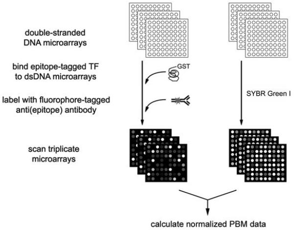
Schema of protein binding microarray experiments. (Reproduced from (Mukherjee et al., 2004) with permission from Nature Publishing Group.)

Figure 2.

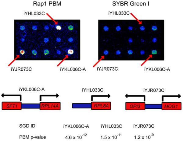
Magnification of identical portions of a yeast intergenic microarrays used in a PBM experiment (left panel) or stained with SYBR Green I (right panel). Fluorescence intensities are shown in false color, with white indicating saturated signal intensity, red indicating high signal intensity, yellow and green indicating moderate signal intensity, and blue indicating low signal intensity. The three labeled spots correspond to the intergenic regions depicted below, along with the P-values derived from triplicate PBM and SYBR Green I microarray data. (Reproduced from (Mukherjee et al., 2004) with permission from Nature Publishing Group.)

Figure 3.

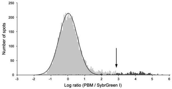
Identification of the DNA binding site motif from the significantly bound spots. (a) Distribution of ratios of PBM data, normalized by SYBR Green I data, for the yeast TF Rap1 bound to yeast intergenic microarrays. The arrow indicates those spots passing a P-value cutoff of 0.001 after correction for multiple hypothesis testing. Indicated in dark gray are spots with an exact match to a sequence belonging to the PBM-derived binding site motif. (b) Sequence logo (Schneider and Stephens, 1990) of the PBM-derived motif for the yeast transcription factor Rap1. (Reproduced from (Mukherjee et al., 2004) with permission from Nature Publishing Group.)

This chapter will describe how to use DNA microarrays in PBM experiments, and how to analyze the resulting microarray data in order to identify the significantly bound spots and the candidate DNA binding site motif. Not discussed in this chapter are methods for protein purification, as there are numerous resources available that provide standard protocols and troubleshooting tips (Coligan et al., 2005). Similarly, methods for printing DNA microarrays are discussed only briefly, as they are described in detail elsewhere (Schena, 1999). Various subsequent analyses that can be performed, such as determining the cross-species conservation of PBM-derived predicted genomic binding sites, comparison of PBM data versus in vivo (ChIP-chip) binding data, and comparison of PBM data with gene expression data, are mentioned only briefly in this chapter, as a detailed discussion of those analyses (Mukherjee et al., 2004) is beyond the scope of this chapter.

Preparation of DNA Microarrays for Use in Protein Binding Microarray Experiments

Overview

The key choice to be made in choosing what DNAs to print onto slides for use in PBM experiments is whether one wishes to synthesize a relatively low complexity microarray for directed experimentation on one or small family of DNA binding proteins (Bulyk et al., 2001), or to synthesize a higher complexity microarray for examination of a broader set of proteins (Mukherjee et al., 2004). Here we describe the latter situation, as the resulting microarrays can be used more broadly, including for uncharacterized proteins. Nevertheless, in certain situations, one might be able to restrict oneself to lower complexity microarrays that consequently are less expensive to produce.

Selection and Preparation of Double-Stranded DNAs (dsDNAs) to be Printed

We have recently used whole-genome yeast intergenic microarrays in PBM experiments in order to identify the DNA binding site specificities of the Saccharomyces cerevisiae TFs Rap1, Abf1, and Mig1 (Mukherjee et al., 2004). These microarrays were printed with essentially all noncoding regions of the S. cerevisiae yeast genome (Ren et al., 2000). Those genomic regions were amplified by PCR, with 25 cycles of 94°C for 30 seconds, 60°C for 30 seconds, and 72°C for 90 seconds. The completed PCR reactions were then precipitated with 1 M ammonium acetate and two volumes of isopropanol, washed with 70% ethanol, dried overnight, and resuspended in 3x SSC printing buffer. After precipitation, the PCR products were resuspended in approximately 15 μl 3x SSC spotting buffer at a concentration between 100 and 500 ng/μl. Alternatively, PCR products may be filtered with a 96-well MultiScreen® PCR Filter Plates (Millipore, Billerica, MA) according to manufacturer's protocols. After application of a vacuum for 10 minutes, plates may be air-dried in a clean chemical hood. The extra filtration provided by the MultiScreen® plates increases the purity of the dsDNA. Other printing buffers or additives such as Sarkosyl or betaine may aid in increasing the spot uniformity and thus improving the morphology of the printed spots. Different slide types will also exhibit different spot morphologies with given printing buffers; care should be taken to ensure that the chosen printing buffer is compatible with the chosen slide type.

Microarrays spotted with coding regions are also expected to aid in identifying the sequence-specific binding properties of DNA binding proteins, despite the fact that it is currently thought that most in vivo functional regulatory sites will be located in noncoding regions. Since PBM experiments are in vitro technology, as long as there is sufficient sequence space represented on the DNA microarrays, one can expect to be able to derive a good approximation of the DNA binding site motif from the PBM data. Since in essence what matters most is the representation of a large enough sequence space on the DNA microarrays, it is actually not necessary to utilize microarrays spotted with amplicons representing genomic regions from the same genome as the DNA binding protein of interest, but rather one can use microarrays spotted with a different genome's sequence. Similarly, microarrays spotted with synthetic dsDNAs can also be used in PBMs. Likewise, the dsDNAs need not be made by PCR amplification, but rather can be made by other means, such as by primer extension. We have successfully performed PBMs using microarrays spotted with PCR products whose lengths ranged from ∼60 to ∼1500 base pairs (Mukherjee et al., 2004), and also using microarrays spotted with synthetic dsDNAs ranging from ∼35 to ∼50 base pairs (Bulyk et al., 2001; Mukherjee et al., 2004).

Printing and Processing of the dsDNA Microarrays

We work with a dedicated microarray facility for production of whole-genome yeast intergenic DNA microarrays for use in our PBM experiments. There, an OmniGrid® 100 microarrayer (Genomic Solutions, Ann Arbor, MI) equipped with Stealth 3 pins (Telechem International, Sunnyvale, CA) is used to spot DNA onto Corning® GAPS II or UltraGAPS 25 × 75 mm amino-silane coated glass slides (Fisher Scientific). Approximately 0.7 nl are deposited at each spot. Any remaining, unused blank GAPS II or UltraGAPS slides from an opened package should be stored in a vacuum desiccator (Fisher Scientific) containing Drierite desiccant (Fisher Scientific). Other slide types could potentially be used. We have found that Corning® GAPS II and UltraGAPS slides result in low slide background in both PBM experiments and staining with SYBR Green I.

After printing, there are a number of options for slide processing protocols. As will be discussed in detail later in this chapter, we have found that spot morphology is very important for achieving high-quality PBM data. We have had success in achieving uniform DNA concentration within spots, as well as round spot morphology, with the following protocol. First, in order to rehydrate the spotted dsDNAs, lay slides face-up and flat, and blow a moisture stream across their surface for approximately 5 seconds using a handheld steam humidifier (Conair, Stamford, CT). Alternatively, one can incubate the microarrays in a humid chamber at 37°C for 48 hours. Next, bake the microarrays in a standard lab oven (VWR International, West Chester, PA) at 80°C for 2 hours. We have found that baking the microarrays at 80°C for 2 hours in a clean oven before UV-crosslinking may improve intra-spot uniformity. However, we caution readers that baking may also result in a decreased shelf life of the microarrays. In order to crosslink the dsDNAs to the slide surface, apply 300 mJ to each slide using a Stratalinker® 1800 UV Crosslinker (Stratagene, La Jolla, CA). Alternatively, amino-modified DNAs could be end-attached to amine-reactive slides, such as PDC slides (Bulyk et al., 2001). The printed, processed slides should be stored in black or orange light-protective plastic slide boxes (Fisher Scientific) placed in a vacuum desiccator equipped with Drierite desiccant.

Staining the dsDNA Microarrays

Staining the dsDNA microarrays serves two purposes: (1) it allows us to check the quality of a given print run; and (2) it allows us to normalize the protein binding data by the relative amount of DNA present at each spot. We routinely stain at least one microarray from each print run and batch of processed slides, in order to assess their quality; for larger printer runs, we will stain one slide from early in the print run, one slide from the middle of the print run, and one slide from late in the print run.

We use SYBR Green I (Molecular Probes, Eugene, OR) to stain the dsDNA microarrays, since SYBR Green I is much more specific for double-stranded versus single-stranded DNA than is ethidium bromide. To prepare the SYBR Green I staining solution, completely thaw the SYBR Green I stock solution at room temperature, in the dark to prevent photobleaching, and then vortex before using. Next, prepare a 1:5000 dilution of SYBR Green I in 2X SSC, 0.1% Triton X-100 (Fisher Scientific), made fresh before use, using sterile water, a stock solution of 10% Triton X-100 (Sigma), filter-sterilized using 0.22 μm filter unit (Fisher Scientific), and stored at room temperature, and a stock solution of 20X SSC, pH 7.0 (Sambrook et al., 1989), sterilized by autoclaving, and stored at room temperature. Unless otherwise noted, buffers are prepared using distilled, deionized water (ddH₂O). If additional slides will be stained within a week, then the prepared SYBR Green I staining solution can be wrapped in aluminum foil, stored at 4°C, and re-used. Mix SYBR Green I staining solution before using to stain microarrays. Since SYBR Green I is light-sensitive, all possible care should be taken to avoid photobleaching in the course of the SYBR Green I staining procedure. We recommend turning off all overhead and benchtop lighting when handling these reagents, and also when handling the microarrays once they have been stained with SYBR Green I. Stain the microarrays with the SYBR Green I staining solution for 12 min by shaking in a Coplin staining jar (Fisher Scientific) for 3 × 1 inch slides at room temperature @ ∼100-125 rpm on a platform shaker. Shaking at speeds faster than ∼125 rpm may cause the Coplin jar to tip over while shaking. Microarrays should be handled with forceps (Fisher Scientific) and gloved hands. Wash the microarrays in 2X SSC, 0.1% Triton X-100 (Fisher Scientific) wash buffer for 5 min, and then in 2X SSC for 2 minutes. All wash steps in Coplin jars are performed by shaking at room temperature @ ∼125 rpm on an adjustable speed platform shaker (Fisher Scientific). Immediately spin slides dry in a table-top centrifuge by centrifuging for 5 min at 40 × g (500 rpm using an IEC Centra CL3R equipped with a 224 Microplate Rotor (Thermo Electron, Milford, MA)).

Before scanning the stained microarrays, wipe the backs (i.e., the non-DNA sides) of the slides with a slightly dampened Kimwipe (Fisher Scientific), in order to remove any streaks or spots due to dried buffer. Very quickly blow any lint off of the spun-dry microarrays using canned air (Fisher Scientific). Scan the microarrays at a range of different laser power intensities or photomultiplier tube (PMT) gain settings per microarray, using an appropriate laser and filter set (for SYBR Green I, an argon ion laser (488 nm excitation) and 522 nm emission filter). We typically scan at ∼3–6 different settings, so as to capture signal intensities for even very low signal intensity spots, while ensuring that we capture sub-saturation signal intensities for all spots on the microarray (Bulyk et al., 2001; Mukherjee et al., 2004). Integrating the data from these multiple scans is described later in this chapter. Using our ScanArray 5000 microarray scanner (Perkin Elmer, Boston, MA), we have found the PMT gain to be optimal at 70-80%. We typically fix the PMT gain setting and vary the laser power in increments of 10-15% of total laser power, so that there are no spots with saturated signal intensities in the lowest intensity scan.

Protein Binding Microarray Experiments

Overview

In PBM experiments, epitope-tagged protein is bound directly to DNA microarrays. It is important to keep in mind the nature of the protein; if a TF is being examined, then one needs to be sure to use dsDNA microarrays. The microarrays can be spotted with either PCR products or with double-stranded DNA oligonucleotides; alternatively, single-stranded oligonucleotide arrays could be made double-stranded in on-array double-stranding reactions (Bulyk et al., 2001). In this chapter, we will describe the use of microarrays spotted with dsDNA, such as the wholegenome yeast intergenic microarrays we used in our PBM experiments on the yeast TFs Rap1, Abf1, and Mig1 (Mukherjee et al., 2004). It is also important to keep in mind that these in vitro experiments are biochemical assays that depend on the reaction conditions; addition of certain small molecule or protein cofactors may be essential for sequence-specific binding by a given protein.

The PBM experiments themselves are neither time-intensive nor laborious, and are readily completed within a single day. Indeed, much of the total experiment time is dedicated to incubations, with only relatively short periods of time being spent on reaction setups, washes, and scanning of the microarrays. Significantly more time is devoted in advance of the PBM experiments to generating the proteins to be bound to the microarrays, and to analysis of the resulting microarray data.

Protein Binding Microarray Experiment Protocol

In order to minimize background, we block the DNA microarrays with a milk solution, and also include milk in both the protein binding and antibody labeling reactions. First, prepare PBS according to standard protocols (Sambrook et al., 1989). Next, prepare 2% and separately 4% nonfat dried milk (Sigma) by dissolving it in PBS with gentle shaking on a platform shaker at 25 rpm, either overnight or for a few hours. Sterilize the 2% and 4% milk solutions with a syringe (Fisher Scientific) equipped with a sterile 0.22 μm filter (Millipore, Billerica, MA) for the 2% milk solution, or with a 0.45 μm filter (Millipore, Billerica, MA) for the 4% milk. Filtering of the 2% and 4% milk solutions serves two purposes: (1) sterilization; and (2) removal of fine particulates that may contribute to speckles in the microarray images. We have found that the 4% milk solution readily clogs a 0.22 μm filter unit, and so we recommend using a 0.45 μm filter unit for syringe-filtering of the 4% milk solution. The 2% milk solution can be syringe-filtered with a 0.22 μm filter. Alternatively, 0.45 μm filters can be used for sterilizing both the 2% and 4% milk solutions.

Before using the DNA microarrays in any reactions, first etch small grooves on the face (i.e., DNA side) of each microarray, at a distance of a few millimeters beyond the borders of the printed area, using a diamond-tipped glass scribe (Fisher Scientific). Microarrays should be handled by their edges with gloved hands or with a forceps; when using forceps either here or in subsequent steps, care should be taken not to scratch the microarray surface. Not only do these etches make it easier for the experimenter in subsequent steps to see where the printed microarray is on the slide surface, but also they will help to confine all solutions to the center portion of the microarray throughout the PBM experiment. Note that border marks made with certain brands of lab markers tend to come off the slides during the various microarray reaction and wash steps.

Prepare pre-wetting buffer (PBS / 0.01% TX-100). For these experiments, make all wash buffers fresh before use. Prepare using a stock solution of 20% Tween-20 (Sigma) or 10% Triton X-100 (Sigma), as indicated, filter-sterilized using 0.22 μm filter unit (Fisher Scientific), and stored at room temperature. Pre-wet the microarrays in PBS / 0.01% TX-100 for at least 5 min by shaking in a Coplin staining jar (Fisher Scientific) at room temperature @ ∼125 rpm on a platform shaker (Fisher Scientific). While the microarrays are being pre-wet, thaw the previously purified DNA binding protein of interest on ice. Purified DNA binding protein, epitope-tagged with glutathione S-transferase (GST), should have been purified according to standard protocols, aliquoted in PBS before storing at −80°C in order to avoid unnecessary freeze/thaw, and stored at -80°C.

Working with one microarray at a time, quickly remove the microarray from the Coplin jar, gently shake off any excess buffer, and wipe the back (i.e., the non-DNA side) and sides of the microarray with a Kimwipe. Drying the back and sides of the microarray with a Kimwipe helps to prevent solution from leaking out from the edges of the cover slip. Because of the hydrophobic surface of the Corning® GAPS II and UltraGAPS glass slides, drying the front of the glass slide outside the perimeter of the DNA spots, using the etched grooves as a guide, can help to confine the protein or antibody solution, once dispensed onto the microarray, to the area of the microarray that contains the DNA spots. This must be done quickly so that the area containing the DNA spots does not dry. Briefly centrifuge all reaction mixtures before applying to microarrays in order to remove bubbles. When pipeting the reaction mixtures onto the microarrays, avoid pipeting any fine bubbles that may remain at the very top surface of the reaction mixtures. If nevertheless a few air bubbles become apparent once a reaction mixture has been applied to a microarray, very carefully attempt to pipet up the bubbles, while avoiding the removal of the reaction mixture. If some air bubbles still remain, they may be brought to the edge of the glass slide, and thus outside the spotted area, by gently rocking the cover slip as it is laid down on the microarray. Apply 250 μl of 2% milk solution (pre-blocking buffer) to the microarrays, cover with a LifterSlips™ cover slip (Erie Scientific, Portsmouth, NH), and allow to incubate in a hydration chamber for 1 hour at room temperature. In applying reaction mixtures onto the microarrays, certain techniques can aid in spreading the mixture over the surface of the microarray, and in increasing the homogeneity of the reaction mixture when applied to a pre-wet or washed microarray. The reaction mixture can be dispensed one droplet at a time, covering the entire surface where the DNA was spotted. The microarray can also be rocked back and forth to spread the reaction mixture uniformly across the spotted area. The use of LifterSlips™ cover slips helps to ensure a uniform distribution of the reaction mixture over the surface of the microarray. Microarrays are incubated in a hydration chamber to prevent excessive evaporation of the reaction mixture under the cover slip. An empty pipet tip box works nicely as a hydration chamber. Lift out the tip rack, fill the bottom of the pipet tip box with about half an inch of sterile water, and replace the tip rack. Wipe off the inside of the lid and the tip rack with ethanol using a Kimwipe before every use and between reaction steps in the PBM experiments.

As soon as the pre-blocking of the microarray has been set up, pre-incubate the DNA binding protein of interest with nonspecific competitors, for 1 hour at room temperature. Specifically, dilute the thawed DNA binding protein to a 20 nM final concentration in a 100 μl protein binding reaction mixture consisting of PBS, 50 μM zinc acetate (ZnAc) (Sigma, St. Louis, MO), 2% (w/v) nonfat dried milk (Sigma), 51.3 ng/μl salmon testes DNA (Sigma), and 0.2 μg/μl bovine serum albumin (New England Biolabs, Beverly, MA). A stock solution of 25 mM ZnAc should be stored in aliquots at −20°C, and then added to various buffers as required; typically ZnAc is necessary only when performing PBM experiments on zinc finger proteins. The final 2% milk concentration is achieved by using a 2-fold dilution of the 4% milk solution that was prepared. A 100 μl reaction volume will be adequate for a printed microarray that encompasses ∼2/3 of a 1× 3 inch slide surface. While the microarrays and the DNA binding protein are pre-blocking separately, thaw Alexa Fluor® 488 conjugated anti-glutathione S-transferase (anti-GST) polyclonal antibody (Molecular Probes) on ice, covered with either an ice bucket lid or aluminum foil, in order to prevent photobleaching. Antibody should be stored according to manufacturer's recommendations. For long-term storage of Alexa Fluor® 488 conjugated anti-GST antibody, we recommend aliquoting and storing at −20°C, per manufacturer's recommendations. Other epitope tags and/or other antibodies conjugated with other fluorophores might also be used successfully. We have not yet performed a rigorous comparison of such alternatives.

Once the 1 hour pre-blocking step is completed, wash the microarrays once with PBS / 0.1% Tween (0.1% Tween-20 in PBS) for 5 min, followed by once with PBS / ZnAc / 0.01 % TX100 (0.01% Triton X-100 in PBS containing 50 μM ZnAc) for 2 min. Wipe the back and sides of the microarrays with a Kimwipe, apply the protein binding reaction mixture to the microarrays, cover with a LifterSlips™ cover slip, and allow to incubate in a hydration chamber for 1 hour at room temperature. As soon as the microarray protein binding reaction has been set up, dilute the Alexa Fluor® 488 conjugated anti-GST antibody to a concentration of 0.05 mg/ml in 2% milk in 150 μl of PBS containing 50 μM ZnAc, and allow to pre-incubate for 1 hour at room temperature in the dark. As with SYBR Green I, all possible care should be taken to avoid photobleaching in the course of staining protein-bound microarrays with Alexa Fluor® 488 conjugated anti-GST antibody.

Once the 1 hour protein binding step is completed, wash the microarrays once in PBS / ZnAc / 0.5% Tween (0.5% Tween-20 in PBS containing 50 μM ZnAc) for 3 min, followed by once in PBS / ZnAc / 0.01% TX100 for 2 min. Wipe the back and sides of the microarrays with a Kimwipe, apply the pre-incubated antibody mixture to the microarrays, cover with a LifterSlips™ cover slip, and allow to incubate in a hydration chamber for 1 hour at room temperature, covered with either an ice bucket or aluminum foil, in order to protect from light.

Once the 1 hour antibody staining is completed, wash the microarrays three times with PBS / ZnAc / 0.05 % Tween (0.05% Tween-20 in PBS containing 50 μM ZnAc), with each wash going for 3 min, followed by once with PBS / ZnAc for 2 min. Immediately spin slides dry in a table-top centrifuge, wipe with KimWipes, and blow any lint off with canned air, as described above under “Staining the dsDNA Microarrays”. Scan the microarrays at a range of different laser power intensities or PMT gain settings per microarray, using an appropriate laser and filter set (for Alexa Fluor™ 488, argon ion laser (488 nm excitation) and 522 nm emission filter), as described above under “Staining the dsDNA Microarrays”.

Analysis of the Protein Binding Microarray Data

Overview

The first step in PBM data analysis is to filter the microarray data in order to remove noisy spots from consideration. Only then are the protein binding data normalized by the SYBR Green I data. From the normalized PBM data, p-values are assigned to each spot in order to identify the significantly bound spots. The sequences corresponding to the significantly bound spots are then searched for candidate DNA binding site motifs with the use of a motif finding algorithm. Additional data analyses, such as the examination of PBM-derived target genes for over-represented functional categories of genes, comparison with ChIP-chip data, cross-species sequence conservation of the predicted binding sites, and prediction of network interactions are beyond the scope of this chapter, and the algorithms for those analyses will likely improve beyond the initial efforts described in (Mukherjee et al., 2004).

Microarray Data Quality Control

If the DNA concentration at a particular spot is too low to allow the accurate quantification of its signal intensity, or if the DNA is spread non-uniformly throughout the pixels of a particular spot, accurate measurements can be more difficult. Obviously problematic microarrays can be identified visually (Fig. 4) (Berger and Bulyk, in press). Severe problems with spot morphology, including non-uniform DNA distribution within the spots, frequently can be attributed to the choice of printing buffer and/or post-printing processing before UVcrosslinking. More subtle differences in spot quality will be identified through analysis of the quantified signal intensity data. It is important to remove error-prone spots from consideration, since the microarray data are subsequently used to estimate the degree of sequence-specific binding of a given DNA binding protein to each spot. Since some spots may be noisy even after removing spots with highly variable pixel signal intensities, we apply various additional filtering criteria to remove them from consideration.

Figure 4.

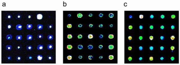
Examples of DNA microarray spot quality. Identical portions of yeast intergenic microarrays printed onto Corning® GAPS II slides, processed in different ways (see below) before UV-crosslinking, and then stained with SYBR Green I. Images have been false-colored as in Figure 2. Examples of microarrays with poor spot quality are shown in (a) and (b). In both of these cases, the DNA is distributed non-uniformly, with either (a) high concentrations near the centers of spots, or (b) high concentrations along spot perimeters. Both of these microarrays resulted from two separate print runs, from which microarrays were UV-crosslinked without first rehydrating and baking. An example of a microarray of acceptable quality is shown in (c). This microarray was rehydrated and then baked before being UV-crosslinked. (Reproduced from (Berger and Bulyk, in press) with permission from The Humana Press, Inc.)

Quantification of the Microarray Signal Intensities and Quality Control

The microarray TIF images are quantified with GenePix Pro microarray analysis software (Axon Instruments, Inc.). Since the PBM experiments are one-color experiments, one can specify in GenePix to analyze the TIF image as a single-color image. Because the images are single-color images that require normalization using data from separate microarrays stained with SYBR Green I, and because even after data filtering spot morphology can still be somewhat variable at times, we recommend keeping the feature size fixed in the GenePix alignment procedure. After image quantification, use Excel, GenePix, or other software to calculate the background-subtracted median intensities; for background, we recommend using the median local background, in order to take into account inhomogeneous background over the microarray.

Because the microarrays were scanned at multiple laser or PMT gain settings in order to capture sub-saturation signal intensity data for as many spots as possible on the microarray, the relative signal intensity data over the full series of scans need to be calculated (Bulyk et al., 2001). To accomplish this task in a semi-automated fashion, we recommend using masliner (MicroArray Spot LINEar Regression) software, which combines the linear ranges of multiple scans from different scanner sensitivity settings onto an extended linear scale (Dudley et al., 2002). The dynamic range of the final PBM and SYBR Green I stained microarrays frequently have post-masliner fluorescence intensities that span 5 to 6 orders of magnitude (Mukherjee et al., 2004).

After masliner analysis, a few normalization procedures are required. First, for microarray data for a given DNA binding protein or SYBR Green I, for each of the triplicate microarrays, remove data corresponding to any flagged spots (i.e., spots that had dust flecks, etc.). Next, normalize the data from each of three triplicate microarrays according to total signal intensity, so that the average spot intensity is the same for all three replicate microarrays. Then, within each individual microarray, separate the data into sectors, according to their local region on the slide. For example, for the whole-genome yeast intergenic arrays (Mukherjee et al., 2004), we sectored the spots into the 32 subgrids of the printed microarray. Normalize the data again so that the mean spot intensity is the same over all the sectors. This serves to normalize for any region-specific inhomogeneities in the background, or the binding and labeling reactions.

After the signal intensity normalization procedures, a number of quality control filtering criteria are applied. We have found that spots with highly variable pixel signal intensities lead to noisy PBM data; therefore, we remove from consideration any spots whose standard deviation (SD) divided by median value is greater than 2. Next, average the background-subtracted, normalized signal intensities for all spots with reliable data in at least two of the three replicate microarrays, and calculate the SD/mean value. In order to eliminate spots that do not have highly reproducible data over the triplicate spots (here, triplicate microarrays since essentially all intergenic regions were printed only once per microarray (Mukherjee et al., 2004; Ren et al., 2000)), we remove from consideration any spots for which the SD/mean value is greater than 1. The SYBR Green I microarray data undergo the same quality control filtering criteria, plus an additional step in which we remove from consideration any spots with fewer than 50% pixels with signal intensities greater than two SDs beyond the median background signal intensity; this additional criterion is applied to the SYBR Green I data, since these spots presumably do not have enough DNA present to allow accurate quantification of signal intensities (Mukherjee et al., 2004), and thus this avoids the problem of dividing by noisy small values in a subsequent normalization (see next section). Although not necessary, we have found empirically that the following three additional filtering criteria helped to eliminate ‘false positive’ calls (i.e., spots with no identifiable binding sites being erroneously identified as bound): (1) DNA length greater than 1500 bp; (2) low SYBR Green I raw signal intensity; and (3) low DNA density (SYBR Green I / length). These three additional filters together removed 2.7% of spots from consideration in our PBM experiments using yeast whole-genome intergenic microarrays (Mukherjee et al., 2004). The actual values for the second and third additional filtering criteria are not provided here, because these values will vary somewhat among individual microarray scanners. We recommend that the user use all three of these additional criteria as suggested guidelines to employ and adjust as may be appropriate (Berger and Bulyk, in press).

Normalization of Protein Binding Signal Intensities by DNA Signal Intensities, and Identification of the Significantly Bound Spots

Once the PBM and SYBR Green I microarray data have been quantified, normalized, and filtered to remove noisy data points, these separate data can then be combined in order to identify the significantly bound spots (Mukherjee et al., 2004). By “significantly bound”, we mean those spots that are bound to a degree beyond that of nonspecific binding by the given protein.

To identify the significantly bound spots, first calculate the log₂ ratio of the mean PBM signal intensity divided by the mean SYBR Green I signal intensity, and create a scatter plot of those log ratios versus the spots' SYBR Green I signal intensities. Although we expect that the log ratio should be independent of DNA concentration, we have found that higher DNA concentrations, as determined by higher SYBR Green I signal intensities, appear to bind proportionately less protein. In order to restore the independence of log ratio and SYBR Green I intensity, fit the scatter plot with a locally weighted least squares regression using the LOWESS function (smoothing parameter = 0.5) (Cleveland and Devlin, 1988) of the R statistics package (www.r-project.org). Then, subtract the value of the regression at each spot from its log ratio, yielding a modified log ratio that is independent of DNA concentration. Next, plot the distribution of all log ratios as a histogram (bin size = 0.05); we expect this distribution to resemble a Gaussian distribution, corresponding to spots bound only nonspecifically, along with a heavy upper tail, which corresponds to the spots bound specifically by the given protein.

We use the large Gaussian-like distribution to calculate P-values for each spot; these P-values represents the probability that the spot is contained within the distribution of nonspecifically bound spots. Thus, spots with very small P-values in the heavy upper tail of the real distribution are likely to be bound sequence-specifically by the given DNA binding protein. We do not use a standard z-score to calculate these P-values, because the heavy upper tail for some proteins can contain quite a number of spots that appear to overlap the right shoulder of the Gaussian-like distribution, thus causing the Gaussian-like distribution to be non-symmetrical. Therefore, we instead calculate a pseudo-z-score to obviate this complication. First, determine the mode of the Gaussian-like distribution by searching for the window of nine bins with the highest number of spots and taking the middle bin. Next, reflect all values less than the mode and fit these values to a Gaussian function using the Mathematica software package (Wolfram Research, Inc., Champaign, IL). This provides the mean and SD of the distribution of nonspecifically-bound spots. Then, adjust the log ratios so that the peak of the distribution of nonspecifically-bound spots is centered on zero. The P-value for each spot is then calculated based on z, the number of SDs that the spot's log ratio departs from the mean of the Gaussian distribution, using the normal error integral (Taylor, 1997). This function is related to the probability of observing a data point greater than z SDs above the mean of a normal distribution. Thus, we are not calculating a true z-score, since here we do not calculate the P-values relative to all the data, but rather just to the reflected left-half of the distribution. These P-values can be calculated easily in Microsoft Excel using the standard normal cumulative distribution function: normsdist(-z).

Finally, the data must be corrected for multiple hypothesis testing (e.g., on an array with 6000 spots, at a significance level of α = 0.001, 6 spots would be expected to be false positives just by chance alone). Therefore, we adjust all individual P-values to a modified significance level using the Modified Bonferroni Method (Bulyk et al., 2002; Sokal and Rohlf, 1995). For significance testing of the PBM data, we recommend using an initial α = 0.001, which corresponds to α' equal to approximately 1.5 × 10⁻⁷ for the highest-ranking test case when evaluating ~6400 unique spots, which is the case for typical yeast intergenic microarray PBM data (Mukherjee et al., 2004). Spots meeting or exceeding α' are considered ‘bound’ at this statistically significant threshold (Fig. 3a). Users may wish to consider spots at less stringent significance thresholds accordingly.

Identification of the DNA Binding Site Motif from the Protein Binding Microarray Data

Once the spots that are bound at a threshold significance level have been identified, then the DNA sequences corresponding to those spots can be searched with one or more motif finding algorithms in order to identify the likely DNA binding site motif of the given protein (Mukherjee et al., 2004). Typically we choose to search the sequences from all the spots that have a Bonferroni-corrected P-value less than or equal to 0.001, in order to minimize consideration of potentially false positive spots that would contribute noise to the motif finding searches. For this set of input sequences, we frequently use BioProspector (Liu et al., 2001) to perform separate motif searches at each width between 6 and 18 nucleotides in order to identify the highest scoring motifs at each width. Other motif finders, such as AlignACE (Hughes et al., 2000; Roth et al., 1998), MEME (Bailey and Elkan, 1995), and MDscan (Liu et al., 2002), can also be used to identify the DNA binding site motif. We tend to choose BioProspector over other available motif finding programs because we have found it to be the most inclusive in accepting the largest number of input sequences in construction of yeast TF binding site motifs (Mukherjee et al., 2004). A graphical sequence logo (Schneider and Stephens, 1990) for each motif is often convenient to have available and can be generated readily (Crooks et al., 2004).

Once a motif has been identified by the given motif finder, we assess the likelihood of it being the DNA binding site motif of the given protein, by considering its group specificity score (i.e., we calculate how specific the motif is to the set of bound spots, as compared to all the spots on the microarray). To perform this calculation, first identify all matches to the motif within all sequences spotted on the microarray using the program ScanACE (Hughes et al., 2000), and then calculate the group specificity score (Hughes et al., 2000) of the discovered motif(s) using MotifStats (Hughes et al., 2000); alternatively, one can perform these same calculations using the software package MultiFinder (Huber and Bulyk, manuscript in preparation). If multiple motifs were discovered for a given dataset, then we choose the single motif with the lowest group specificity score (i.e., most specific to the input set of spots) as the most likely TF binding site motif. In order to assess the statistical significance of the motifs resulting from analysis of the PBM experiments, repeat these calculations for computational negative control sequence sets. Specifically, perform identical motif searches on 10 separate sets of randomly selected spots from the same microarrays used for the PBM experiments, with each of the 10 random sets containing the same number of sequences as the original input set for the given PBM dataset. We consider PBM-derived motifs with group specificity scores that are more significant than the group specificity scores of the corresponding computational negative control sets to correspond to the DNA binding site motif for the given DNA binding protein (Fig. 3b). Examples of the ranges of group specificity scores for computational negative controls and for actual PBM data for yeast TFs can be found in (Mukherjee et al., 2004).

Conclusions

PBM binding site data on the TFs Rap1, Abf1, and Mig1, determined using whole-genome S. cerevisiae intergenic microarrays, corresponded well (Mukherjee et al., 2004) with binding site specificities determined from ChIP-chip (Lee et al., 2002; Lieb et al., 2001). Furthermore, comparative sequence analysis of the PBM-derived binding sites indicated that many of the sites identified as bound in PBMs, including some not identified as bound in the ChIP-chip data, are highly conserved in other sensu stricto yeast genomes and thus are likely to be functional in vivo binding sites that may be utilized in a condition-specific manner (Mukherjee et al., 2004). Further comparisons of these data types may reveal local sequence context features that govern binding site usage in vivo. Improved data analysis algorithms may help to more precisely identify both the significantly bound spots, and their biological relevance.

Looking beyond yeast, at this time the DNA binding specificities of a large majority of metazoan TFs have not yet been characterized. PBM experiments may help to assign functions for these proteins, by determining their DNA binding specificities, and thus predicting their target regulated genes. For example, in analyzing the Gene Ontology (GO) annotation of the PBM-predicted target genes for Rap1, Abf1, and Mig1, we observed highly significant enrichment of functional categories that are consistent with the known regulatory roles of these TFs (Mukherjee et al., 2004). There are hundreds of Drosophila TFs, and thousands of mammalian TFs, that could be examined in this manner. Likewise, a number of uncharacterized target genes were predicted as target genes of these yeast TFs; one may also be able infer the biological process that these predicted target genes are involved in, from the functions of the given TF. Integration of gene expression data with the PBM data and GO annotations may allow the refinement of these regulatory and functional predictions, including predictions regarding in which environmental conditions a given TF is exerting an important regulatory role.

Importantly, like any other microarray experiment, multiple PBM experiments can be performed in parallel, allowing many proteins to be examined on a genome scale at once. Alternatively, instead of intergenic microarrays, one could instead create microarrays spotted with a large number of synthetic DNA sequence variants, in order to examine protein-DNA interactions at a higher sequence resolution. The highly parallel nature of microarray experiments, both in terms of the spotted DNAs and the number of microarray experiments that can be performed simultaneously, provides significant cost, time, and labor savings over the use of traditional methods for examining protein-DNA interactions. The resulting data will likely contribute to the elucidation of transcriptional regulatory networks in a variety of genomes. In addition, these data may allow us to glean insights on the biophysical properties that determine protein-DNA recognition specificity. Finally, analysis of PBM data for orthologous TFs of various phylogenetic distances may provide insights into the evolution of binding sites and thus the TFs' species-specific regulatory roles.

References

- Bailey T, Elkan C. The value of prior knowledge in discovering motifs with MEME. Proc. Int. Conf. Intell. Syst. Mol. Biol. 1995;3:21–9. [PubMed] [Google Scholar]
- Berger MF, Bulyk ML. Protein binding microarrays (PBMs) for the rapid, high-throughput characterization of the sequence specificities of DNA binding proteins. In: Bina M, editor. Gene mapping, discovery, and expression. The Humana Press, Inc.; Totowa, New Jersey: in press. [Google Scholar]
- Braun P, LaBaer J. High throughput protein production for functional proteomics. Trends Biotechnol. 2003;21:383–8. doi: 10.1016/S0167-7799(03)00189-6. [DOI] [PubMed] [Google Scholar]
- Bulyk M. Computational prediction of transcription-factor binding site locations. Genome Biol. 2003;5:201. doi: 10.1186/gb-2003-5-1-201. [DOI] [PMC free article] [PubMed] [Google Scholar]
- Bulyk M, Johnson P, Church G. Nucleotides of transcription factor binding sites exert interdependent effects on the binding affinities of transcription factors. Nucleic Acids Res. 2002;30:1255–61. doi: 10.1093/nar/30.5.1255. [DOI] [PMC free article] [PubMed] [Google Scholar]
- Bulyk ML, Huang X, Choo Y, Church GM. Exploring the DNA-binding specificities of zinc fingers with DNA microarrays. Proc. Natl. Acad. Sci. USA. 2001;98:7158–63. doi: 10.1073/pnas.111163698. [DOI] [PMC free article] [PubMed] [Google Scholar]
- Cleveland W, Devlin S. Locally weighted regression: An approach to regression analysis by local fitting. J. American Statistical Association. 1988;83:596–610. [Google Scholar]
- Coligan J, Bunn B, Speicher D, Wingfield P, Ploegh H. Current Protocols in Protein Science. John Wiley & Sons, Inc.; Edison, NJ: 2005. [Google Scholar]
- Crooks GE, Hon G, Chandonia JM, Brenner SE. WebLogo: a sequence logo generator. Genome Res. 2004;14:1188–90. doi: 10.1101/gr.849004. [DOI] [PMC free article] [PubMed] [Google Scholar]
- Dudley A, Aach J, Steffen M, Church G. Measuring absolute expression with microarrays with a calibrated reference sample and an extended signal intensity range. Proc. Natl. Acad. Sci. U.S.A. 2002;99:7554–7559. doi: 10.1073/pnas.112683499. [DOI] [PMC free article] [PubMed] [Google Scholar]
- Hughes JD, Estep PW, Tavazoie S, Church GM. Computational identification of cis-regulatory elements associated with groups of functionally related genes in Saccharomyces cerevisiae. J. Mol. Biol. 2000;296:1205–14. doi: 10.1006/jmbi.2000.3519. [DOI] [PubMed] [Google Scholar]
- Lee T, Rinaldi N, Robert R, Odom D, Bar-Joseph Z, Gerber G, Hannett N, Harbison C, Thompson C, Simon I, Zeitlinger J, Jennings E, Murray H, Gordon D, Ren B, Wyrick J, Tagne J, Volkert T, Fraenkel E, Gifford D, Young R. Transcriptional regulatory networks in Saccharomyces cerevisiae. Science. 2002;298:799–804. doi: 10.1126/science.1075090. [DOI] [PubMed] [Google Scholar]
- Lieb JD, Liu X, Botstein D, Brown PO. Promoter-specific binding of Rap1 revealed by genome-wide maps of protein-DNA association. Nat. Genet. 2001;28:327–34. doi: 10.1038/ng569. [DOI] [PubMed] [Google Scholar]
- Liu X, Brutlag D, Liu J. BioProspector: discovering conserved DNA motifs in upstream regulatory regions of co-expressed genes. Pac. Symp. Biocomput. 2001:127–38. [PubMed] [Google Scholar]
- Liu X, Brutlag D, Liu J. An algorithm for finding protein–DNA binding sites with applications to chromatin-immunoprecipitation microarray experiments. Nat. Biotechnol. 2002;20:835–9. doi: 10.1038/nbt717. [DOI] [PubMed] [Google Scholar]
- Lockhart DJ, Winzeler EA. Genomics, gene expression and DNA arrays. Nature. 2000;405:827–36. doi: 10.1038/35015701. [DOI] [PubMed] [Google Scholar]
- Mukherjee S, Berger MF, Jona G, Wang XS, Muzzey D, Snyder M, Young RA, Bulyk ML. Rapid analysis of the DNA-binding specificities of transcription factors with DNA microarrays. Nat. Genet. 2004;36:1331–9. doi: 10.1038/ng1473. [DOI] [PMC free article] [PubMed] [Google Scholar]
- Ren B, Robert F, Wyrick JJ, Aparicio O, Jennings EG, Simon I, Zeitlinger J, Schreiber J, Hannett N, Kanin E, Volkert TL, Wilson CJ, Bell SP, Young RA. Genome-wide location and function of DNA binding proteins. Science. 2000;290:2306–9. doi: 10.1126/science.290.5500.2306. [DOI] [PubMed] [Google Scholar]
- Roth FP, Hughes JD, Estep PW, Church GM. Finding DNA regulatory motifs within unaligned noncoding sequences clustered by whole-genome mRNA quantitation. Nat. Biotechnol. 1998;16:939–45. doi: 10.1038/nbt1098-939. [DOI] [PubMed] [Google Scholar]
- Sambrook J, Fritsch E, Maniatis T. Molecular Cloning: A Laboratory Manual. Cold Spring Harbor Laboratory Press; Cold Spring Harbor, NY: 1989. [Google Scholar]
- Schena M. DNA Microarrays: A Practical Approach. Oxford University Press; New York, NY: 1999. [Google Scholar]
- Schneider TD, Stephens RM. Sequence logos: a new way to display consensus sequences. Nucleic Acids Res. 1990;18:6097–6100. doi: 10.1093/nar/18.20.6097. [DOI] [PMC free article] [PubMed] [Google Scholar]
- Sokal R, Rohlf R. Biometry: The Principles and Practice of Statistics in Biological Research. W. H. Freeman and Company; New York: 1995. [Google Scholar]
- Taylor J. An Introduction to Error Analysis. University Science Books; Sausalito, CA: 1997. [Google Scholar]
- Zhu H, Bilgin M, Snyder M. Proteomics. Annu. Rev. Biochem. 2003;72:783–812. doi: 10.1146/annurev.biochem.72.121801.161511. [DOI] [PubMed] [Google Scholar]