Sampling the Spatial Patterns of Cancer: Optimized Biopsy Procedures for Estimating Prostate Cancer Volume and Gleason Score

Abstract

Prostate biopsy is the current gold-standard procedure for prostate cancer diagnosis. Existing prostate biopsy procedures have been mostly focusing on detecting cancer presence. However, they often ignore the potential use of biopsy to estimate cancer volume (CV) and Gleason Score (GS, a cancer grade descriptor), the two surrogate markers for cancer aggressiveness and the two crucial factors for treatment planning. To fill up this vacancy, this paper assumes and demonstrates that, by optimally sampling the spatial patterns of cancer, biopsy procedures can be specifically designed for estimating CV and GS. Our approach combines image analysis and machine learning tools in an atlas-based population study that consists of three steps. First, the spatial distributions of cancer in a patient population are learned, by constructing statistical atlases from histological images of prostate specimens with known cancer ground truths. Then, the optimal biopsy locations are determined in a feature selection formulation, so that biopsy outcomes (either cancer presence or absence) at those locations could be used to differentiate, at the best rate, between the existing specimens having different (high v.s. low) CV/GS values. Finally, the optimized biopsy locations are utilized to estimate whether a new-coming prostate cancer patient has high or low CV/GS values, based on a binary classification formulation. The estimation accuracy and the generalization ability are evaluated by the classification rates and the associated receiver-operating-characteristic (ROC) curves in cross validations. The optimized biopsy procedures are also designed to be robust to the almost inevitable needle displacement errors in clinical practice, and are found to be robust to variations in the optimization parameters as well as the training populations.

1. Introduction

1.1. The Need for Estimating Surrogate Markers for Cancer Significance

In an aging population, prostate cancer continues to be the second leading cause for cancer-related death in American men. In the year 2008 alone, the American Cancer Society estimated 186,320 incidences and 28,660 mortalities of prostate cancer in the United States [1]. The disparity between cancer incidence and the associated mortality rates implies that, although prostate cancer is the most common cancer in US men, only a small proportion of prostate cancer cases will be life-threatening [22]. Those life-threatening prostate cancers are often known as “clinically-significant” prostate cancers, which are loosely defined as cancers that are rapidly growing, aggressively infiltrating the surrounding normal tissue and/or highly likely to spread to other parts of the body [3, 43, 44]. Indeed, clinical significance of prostate cancer is the primary factor for clinical decision-makings: those patients with clinically-significant prostate cancer should be followed with immediate treatment; whereas those with clinically-insignificant prostate cancer should be only followed with watchful waiting. Therefore, accurate evaluation of cancer significance becomes crucial for effective cancer management.

Evaluation of cancer significance is a challenging task, since it requires accurate identification of prostate cancer and accurate assessment of cancer spatial extent. Generally, cancer significance can be evaluated either directly or indirectly; while the direct way is ideal, it is the indirect way that is more practical and that we will follow in this paper. Actually, the direct way is to carefully examine the cancer prognosis in a series of longitudinal follow-ups. However, this is often impractical, mostly due to its long study time and high clinical cost, and due to the lack of a diagnostic tool that can accurately identify cancer in vivo. In the absence of longitudinal follow-ups, clinical practice often follows the indirect way – to estimate certain surrogate markers at one time instance, and use the estimated surrogate markers to indirectly evaluate cancer significance. The commonly-used surrogate markers include cancer volume, stage, grade, age, genetic factors and ethnic factors. Of those, two surrogate markers are perhaps most important: cancer volume and Gleason Score (a cancer grade descriptor scored 2–10, higher score indicating more aggressive cancer and worse prognosis [19]). This paper follows this indirect way of evaluating cancer significance and aims to improve the estimation accuracy for cancer volume (CV) and Gleason Score (GS), the two most important surrogate markers.

1.2. Existing Methods

Currently, estimation of CV and GS relies on either imaging techniques (e.g., [18, 2, 10, 25]) or biopsy procedures (e.g. [24, 44, 27, 7, 45, 42, 49]). Although imaging techniques, especially the fast-evolving magnetic resonance imaging (MRI), have the advantage in their non-invasive nature, they suffer greatly from the modest sensitivity and specificity, a drawback that is commonly recognized in the prostate imaging literature (e.g., [25, 28]). In the absence of an imaging modality that could accurately and reliably diagnose prostate cancer at the current stage, prostate biopsy continues to be the standard procedure for estimating CV/GS. Generally, biopsy estimates CV/GS by sampling the prostate at a number of locations via biopsy needles. The biopsy-sampled prostate tissue then undergoes microscopic examinations, revealing cancer presence/absence and cancer pathology. However, as addressed below, using existing biopsy procedures to estimate CV/GS is often limited in two respects.

First, the sampling locations in the current biopsy procedures are often suboptimal. In most biopsy procedures, the sampling locations are determined in a random or empirical manner, leading to mis-detection of cancer and mis-estimation of surrogate markers [30, 14]. To cope with that, several computer-assisted approaches (e.g., [45, 42, 49]) have been developed. Their approaches maximized the probability of biopsy needles to intersect with cancerous tissue, and hence remarkably improved the detection of cancer presence. However, they are not necessarily optimal for the estimation of surrogate markers like CV and GS, since for the estimation of CV/GS, the limited number of biopsy needles has to not just intersect with cancerous tissue, but also represent the spatial extent and pattern of cancer in the whole prostate. This requirement renders the use of biopsy for CV/GS estimation fairly challenging.

Second, the traditional criteria for surrogate marker estimation are often suboptimal. For estimating CV, the traditional criterion is the percentage of positive biopsies (e.g. [40]) – more positive biopsies needles indicate larger cancers. This criterion, although quite intuitive, may fail in certain circumstances. As illustrated in Fig. 1, it will incorrectly yield the same percentage of positive biopsies (2 out of 6 in this case) for two prostates whose CV values are substantially different. A possible solution to this problem would be increasing the number of sampling locations, as suggested in [44, 46], but that would substantially increase patient pain, and moreover it might increase our risk of detecting clinically-insignificant prostate cancers, leading to unnecessary treatment and all pertinent side effects [27]. For estimating GS, on the other hand, the traditional criterion is to analyze the limited number of prostate tissue samples extracted by biopsy, find out two most common glandular cancer patterns from those limited tissue samples, assign to each of them a Gleason Grade (ranging from 1–5) and subsequently add the two Gleason Grades together [19]. However, several studies (e.g. [8, 31]) pointed out that the biopsy estimated Gleason Score (usually known as “clinical Gleason Score”, or cGS) is often different from the actual Gleason Score obtained after the prostate removal (usually known as “pathological Gleason Score”, or pGS). In other words, using biopsy-extracted cGS to estimate the actual pGS is subject to mis-estimations. And worse, such mis-estimation might be substantial in a considerable proportion of cases [26]. To minimize mis-estimations for both CV and GS, an ideal estimation criterion should comprehensively consider the biopsy outcomes from all biopsy locations, in a sophisticated, perhaps highly non-linear way that could effectively reflect the spatial pattern of cancer. Actually, this novel, cancer-spatial-pattern-based estimation criterion is one of the major contributions in our study, as will be addressed later in this section.

Figure 1.

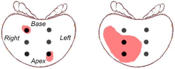
A typical scenario where mis-estimation occurs when using the commonly-adopted estimation criterion for CV. Black solid dots represent the biopsy locations in clinical routines. The red regions represent prostate cancer regions. Please refer to text for more details.

1.3. The Proposed Method

This paper presents optimized biopsy procedures specifically designed for estimating cancer volume (CV) and Gleason Score (GS), two of the most important surrogate markers for the clinical significance of prostate cancer. In our study, the estimation for CV/GS is binary (high v.s. low) instead of continuously-valued, so as to better relate to the clinical decisions that tend to be binary: immediate treatment for CV/GS values above certain clinical threshold, or “watchful waiting” otherwise.

Our approach assumes that, prostate cancers having different (high v.s. low) CV/GS values may exhibit different spatial patterns, which could be properly sampled by optimally-placed biopsy needles. By “spatial pattern”, we mean spatial distribution of cancer reflected by the biopsy outcomes at all sampling locations. For instance, if we order the biopsy locations in Fig. 1 from base to apex, right to left, and denote the biopsy outcome at each biopsy location to be 1 for cancer positive and 0 otherwise, we will observe spatial cancer pattern of [1 0 0 0 0 1] for the first patient and [0 1 1 0 0 0] for the second patient. In this way, CV values of those two patients could be effectively estimated/differentiated, because the pattern of two positive biopsies next to each other (in the second patient) most probably implies cancer distributed in a larger, connected area than the pattern of two positive biopsies far apart (in the first patient). Actually, as will be demonstrated both qualitatively in Section 2.3 and quantitatively in Section 3.2, the spatial pattern of cancer is a robust estimation criterion with consistent high estimation accuracy in the population under study.

Based on the assumption of using spatial cancer pattern for estimation, our approach combines image analysis and pattern classification tools in a statistical atlas-based population study. To learn the differences of spatial cancer patterns between the subpopulations having different (high v.s. low) CV/GS values, our approach first constructs statistical cancer atlases from histological images of a cohort of surgically-extracted prostate specimens. Then, the optimal biopsy locations are determined in a feature selection formulation, so that biopsy outcomes (either cancer presence or absence) at those locations could altogether differentiate between the subpopulations of high and low CV/GS specimens at the best rate. The optimized biopsy locations are thereafter used to estimate whether a new-coming prostate cancer patient has high or low CV/GS values, in a SVM-based binary classification formulation. The estimation accuracy and the generalization ability of our approach are evaluated by the classification rates and the associated receiver-operating-characteristic (ROC) curves in cross validations.

Compared with optimized biopsy procedures previously developed in [45, 42, 49], our approach has the following three merits. The first and foremost merit lies in the objective: previous ones aim to improve the detection of cancer presence; ours aims to estimate surrogate markers for the clinical significance of prostate cancer, which is a far more important yet far more difficult problem. Detecting cancer presence, the objective in their studies, requires that at lease one biopsy needle intersects with cancer; whereas estimating surrogate markers, the objective in our study, has an additional requirement – it requires biopsy needles to sample the prostate in a way that can reflect the spatial cancer patterns. The second merit is the high generalization ability in our approach. The high generalization ability stems from the sparsity of SVM in the feature selection and pattern classification formulations; it also arises from using the novel, more reliable spatial-pattern-based estimation criterion in the classification formulation. The third merit of our approach is its robustness to the almost inevitable uncertainties of needle placement in clinical practice. The robustness is obtained by selecting optimized biopsy locations that have high estimative powers not only at themselves but also in their neighborhoods. Moreover, unlike many optimization processes, whose performances are heavily dependent on the optimization parameters being used, our biopsy optimization process is relatively stable in terms of estimation accuracy, regardless of the variations in the optimization parameters and the training populations, as will be shown in the sensitivity analysis in Section 4.

The remainder of this paper is organized as follows. Section 2 details our framework. Section 3 shows the results for the optimized biopsy procedures and their estimation/classification accuracies. Section 4 examines the robustness of our framework with regard to the variations in the optimization parameters and training populations. Finally, Section 5 discusses and concludes this paper.

2. Method

2.1. General Framework

As sketched in Fig. 2, our approach consists of three components: atlas construction (via image registration), biopsy location optimization (via feature selection) and surrogate marker estimation based on the optimized biopsy locations (via binary classification). Those three components are elaborated in the subsequent Sections 2.3–2.5. Prior to that, we will first describe data acquisition in Section 2.2.

Figure 2.

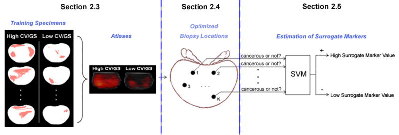
Systematic sketch for the general framework of our approach.

2.2. Data Acquisition

We have collected a population of 83 prostate specimens {p_n|n = 1, 2, …, N} (N = 83) that have undergone radical prostatectomy (a surgery for prostate removal). These specimens are available from the tissue bank of the Center for Prostate Disease Research (CPDR) (http://www.cpdr.org). They are aged 60.4±6.3 years old (min 44, max 73), with pre-biopsy prostate-specific antigen (PSA) values at 12.59 ± 18.52 ng/mL (min 0.7, max 138), and the actual prostate sizes at 92.7±41.1 grams (min 46, max 165, 1 gram in weight is approximately equal to 1 cc in volume).

Those specimens are further divided into different subpopulations, according to surrogate marker values that are known from pathological analysis. When different surrogate marker is used, the subpopulation division might be different. Specifically, when CV/GS is the surrogate marker under estimation, those specimens are divided into a subpopulation of 46/47 specimens with high CV/GS and the remaining 37/36 with low CV/GS. Here, the thresholds of 0.5cc for CV and 6 for GS are adopted from clinical conventions. After the division, each specimen p_n is assigned with a class label C(p_n),

$$C(p_n)=\{\begin{array}{ll}+1\hfill & \text{if}{p}_n\text{has}\text{high}\text{surrogate}\text{marker}\text{value}\hfill \\ -1\hfill & \text{otherwise.}\hfill \end{array}$$ (1)

As shown in Table 1, the subpopulation divisions have uncovered three interesting facts that are worth noting. First, almost one quarter of the specimens have low CV and low GS, an indication that their cancers might be clinically-insignificant. This is a fundamental issue in clinical practice: some patients may be detected with cancer by repeated biopsies; however, their cancers might be insignificant so that they should not be followed with prostatectomy. This fact underlines the importance of estimating their surrogate markers and clinical significance as what we are discussing in this paper. Second, being high in one surrogate marker does not necessarily indicate being high in the other (19.3% has high GS but low CV, while 18.1% has low GS but high CV). Therefore, the class labels for a same specimen might be different when different surrogate markers are under estimation. For the same reason, different atlases and different optimized biopsy procedures are needed for estimating different surrogate markers. Third, overall, the prostate specimens having high and low surrogate markers in our study are almost half and half (or, more accurately, 56% and 44%), so the dataset is not noticeably biased when it is used to reflect different cancer patterns in subpopulations having different CV/GS values.

Table 1.

Number of specimens in the subpopulations having high or low CV/GS. The thresholds (0.5cc for CV and 6 for GS) are adopted from clinical conventions.

	High CV (≥0.5cc)	Low CV (<0.5cc)	Total
High GS (≥6)	31 (37.3%)	16 (19.3%)	47 (56.6%)
Low GS (<6)	15 (18.1%)	21 (25.3%)	36 (43.4%)
Total	46 (55.4%)	37 (44.6%)	83 (100%)

To also present pathologists-defined cancer ground truth, histological images have been collected for all specimens. During the histology collection, each specimen was whole-mounted, step-sectioned at 2.25mm intervals and H/E stained at 5 μm thickness, leading to series of 2D histological slices with pathologically-defined cancer ground truth (e.g. red regions in Fig. 3); then, the series of 2D histological slices were reconstructed into a 3D histological image, which will be used to reveal 3D cancer distributions in the subsequent atlas constructions.

Figure 3.

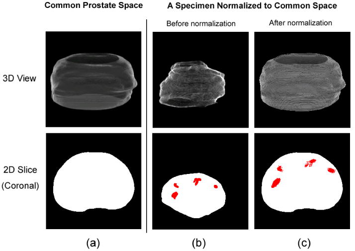
The common prostate space (a) and the histological image of a typical specimen before (b) and after (c) the 3D spatial normalization, in both 3D (top row) and 2D (bottom row) views. Red regions are cancer ground truths labeled by pathologists. The bottom row shows the central slice in the coronal orientation.

2.3. Constructing Statistical Atlases

From those acquired population data, our study first constructs statistical atlases to observe the different cancer spatial patterns from subpopulations having different surrogate marker values. This will provide qualitative support for using the spatial pattern of cancer as a reliable estimation criterion. Generally, a statistical atlas is a model of the object/organ of interest, usually represented as the probability of certain anatomic structure or certain types of tissue (in our paper, cancerous tissue) being present at each voxel in the 3D coordinate system [42, 15, 37, 9].

Basis to the atlas construction is to spatially normalize the 3D histological images across specimens into a common prostate space S, which has regular shape and has 256 × 256 × 124 image voxels. The spatial normalization is done by a 3D surface-based non-rigid image registration method [41]. Fig. 3 shows the common prostate space and a typical histological image before and after the spatial normalization, in both 3D and 2D views. The spatial normalization preserves the zonal anatomy of the prostate, as demonstrated in [49], so that after normalization, the same spatial coordinates will correspond to approximately the same anatomic locations across specimens.

Then, the statistical cancer atlases are constructed by merging the spatially-normalized histological images for each subpopulation. Results are shown in Fig. 4. In the atlases, the brightness of each voxel represents the probability of cancer occurrence in the subpopulation of interest. From visual inspections, it is not difficult to observe that, statistically, subpopulations having different surrogate marker values do exhibit different spatial patterns (distributions) of caner. Moreover, some candidate biopsy locations (e.g., blue dots in Fig. 4) can be intuitively observed, since biopsy outcomes (either cancer positive or negative) at those locations would most probably differentiate between different subpopulations. How to automatically and accurately select the optimal biopsy locations is described in the following sub-sections.

Figure 4.

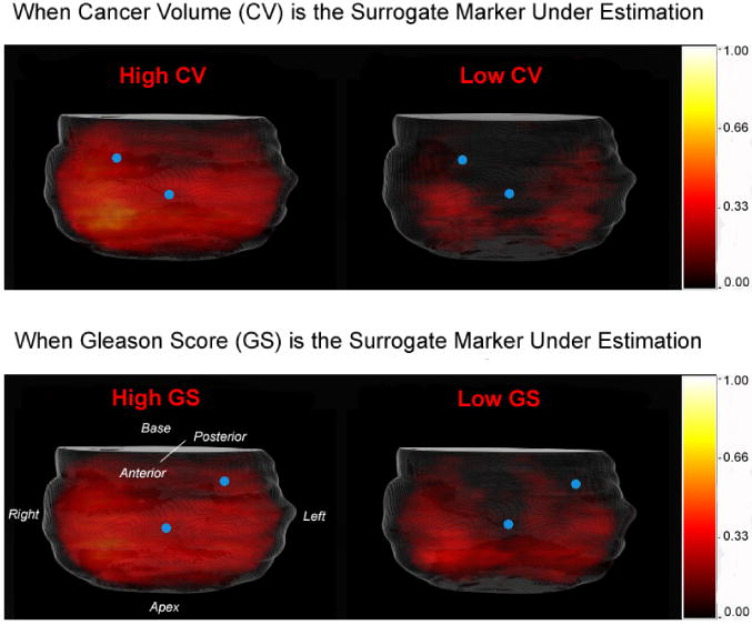
Statistical atlases constructed from subpopulations having different (high v.s. low) surrogate marker values. Blue dots represent intuitively-observed biopsy locations where different subpopulations can be differentiated.

2.4. Determining Optimal Biopsy Locations by Feature Selection

In this section, the problem of selecting optimal biopsy locations is converted to a feature selection formulation. Basis to this conversion is the feature extraction step, which connects each potential biopsy location in the common prostate space with a feature in the feature space.

2.4.1. Feature Extraction: Connecting Each Potential Biopsy Location to a Feature

A potential biopsy location u ∈ S ⊂ ℜ³ is connected to a feature B(u), provided that B(u) is the “biopsy outcome” of the biopsy needle centered at location u. This connection is further explained below.

Mathematically, a biopsy needle can be modeled as a semi-cylinder Q(O),

$$Q(\text{O})=\{(x,y,z)|\sqrt{{(x-O_x)}^2+{(y-O_y)}^2}\le r,0\le y-O_y\le r,\Vert z-O_z\Vert \le l\}$$ (2)

where O = (O_x, O_y, O_z) ∈ ℜ³ is the center, r is the base radius and l is the semi-length of the semi-cylinder (c.f. Fig. 5). Since r = 1.5mm and l = 6mm are usually determined from clinical conventions, the semi-cylinder shaped biopsy model has only one parameter – the center O.

Figure 5.

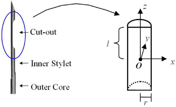
Modeling a biopsy needle as a semi-cylinder. (a) A typical biopsy needle – when it is placed into the prostate, the “cut-out” part will extract a piece of prostate tissue; (b) the cut-out part of the biopsy is modeled as a semi-cylinder, with center O, base radius r and semi-length l. The values of r = 1.5mm and l = 6mm are determined by clinical conventions.

When this semi-cylinder shaped biopsy needle is centered at a potential biopsy location u ∈ S ⊂ ℜ³, it will extract a piece of prostate tissue also centered at u. From an image analysis point of review, the extracted piece of prostate tissue can be modeled as

$$\text{Tissue}(\text{u})=Q(\text{u})\cap S.$$ (3)

This piece of prostate tissue will exhibit either cancer presence or cancer absence, denoted as “biopsy outcome” B(u),

$$B(\text{u})=\{\begin{array}{ll}1\hfill & \text{if}\text{cancer}\text{present}\text{in}\text{Tissue}(\text{u})\hfill \\ 0\hfill & \text{otherwise}\hfill \end{array}$$ (4)

In this way, each specimen p_n can be represented by a high-dimensional feature vector F(p_n; {u₁, u₂, …, u_M}), i.e.,

$$F(p_n;\{{\text{u}}_1,{\text{u}}_2,\dots ,{\text{u}}_M\})=[B_{p_n}({\text{u}}_1),B_{p_n}({\text{u}}_2),\dots ,B_{p_n}({\text{u}}_M)],$$ (5)

where u₁, u₂, …, u_M are all possible biopsy locations, with M being the total number of them. The connection between each potential biopsy location and a feature is also illustrated in Fig. 6.

Figure 6.

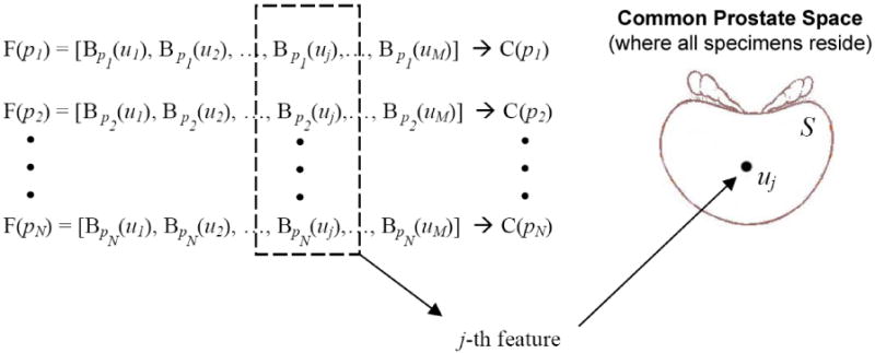
Feature extraction step connects each potential needle location u_j with a feature B(u_j). This connection is the basis to the conversion of the problem of selecting optimal biopsy locations into the feature selection formulation.

2.4.2. Feature Selection: Finding Optimized Biopsy Locations

After connecting each potential biopsy location u with a feature B(u) in the feature extraction step, it naturally follows that the problem of selecting K optimal biopsy locations {u_s1, u_s2, …, u_sK} in the common prostate space S can be translated to the selection of a subset of K best features {B(u_{s1}), B(u_{s2}), …, B(u_{sK})} in the feature space, i.e.,

$$f(p_n;\{s_1,s_2,\dots ,s_K\})=[B_{p_n}({\text{u}}_{s_1}),B_{p_n}({\text{u}}_{s_2}),\dots ,B_{p_n}({\text{u}}_{s_K})],$$ (6)

such that under certain classifier whose decision function is Z[·], the classification result Z[f (p_n; {s₁, s₂, …, s_K}] could agree with pre-known class label C(p_n) at the best rate, for all specimens n = 1, 2, …, N, i.e.,

$$\{s_1,s_2,\dots ,s_K\}=\text{arg}\underset{\begin{array}{c}\{t_1,t_2,\dots ,t_K\}\\ \subset \{1,2,\dots ,M\}\end{array}}{\text{min}}{\sum _{n=1}^N\Vert Z[f(p_n;\{t_1,t_2,\dots ,t_K\})]-C(p_n)\Vert }_{L_1}$$ (7)

Here f (p_n; {t₁, t₂, …, t_K}) denotes the biopsy-extracted multivariate information (spatial-pattern-vector) at those K locations {t₁, t₂, …, t_K} from training prostate specimen p_n.

2.4.3. Solving the Feature Selection Problem

Selecting K out of M features is a challenging task when we have K ≪ M in our problem. Indeed, K, the number of optimal biopsy locations, is typically ranged from 6 to 12 (keep in mind that, in order to reduce patient pain and the biopsy-induced morbidities, a small K value is usually preferred). Meanwhile, when the image space is discretized, M, the total number of all possible biopsy locations, is usually in the millions.

Feature selection methods have been extensively investigated in the machine learning community. Their common purpose is often to determine a small number of optimal features for increasing both the accuracy and the generalization ability of classification. During the past two decades, a variety of methods have been developed for feature selection, such as Adaboost [16] and decision trees [38]. In [20], Guyon and Elisseeff summarized that the most frequently used feature selectors can be broken down into two types: feature ranking and subset selection. They both have merits and drawbacks. Particularly, feature ranking methods rank features according to their individual predictive powers and simply pick up a number of top-ranked features – this type of methods are computationally economic, but will often lead to highly sub-optimal solutions, as they do not evaluate the statistical correlations among features. Subset selection methods, on the other hand, select a subset of features that altogether have the highest predictive power – this type of methods will lead to globally optimal solutions, but are often time-consuming or even computationally prohibitive when the total number of features is large, as in our case. In practice, these two types of feature selectors are often jointly used: to initialize with feature ranking and to refine with subset selection. We adopt this two-step strategy in our approach.

Step 1: Feature Ranking

Features are first ranked by their individual estimative powers. The estimative power of the i^th feature (hence the potential biopsy location u_i) is measured by the Pearson's correlation coefficient with class labels C(p_n) across all specimens p_n(n = 1, 2, …, N), i.e.,

$$\rho ({\text{u}}_i)=\frac{{\sum }_{n=1}^N\left(B_{p_n}({\text{u}}_i)-\overline{B}({\text{u}}_i)\right)\left(C(p_n)-\overline{C}\right)}{\sqrt{\left[{\sum }_{n=1}^N{\left(B_{p_n}({\text{u}}_i)-\overline{B}({\text{u}}_i)\right)}^2\right]\left[{\sum }_{n=1}^N{\left(C(p_n)-\overline{C}\right)}^2\right]}},$$ (8)

Here $\overline{B}({\text{u}}_i)=\frac{1}{N}{\sum }_{n=1}^N{B}_{p_n}({\text{u}}_i)$ is the mean biopsy outcome at location u_i across all specimens and $\overline{C}=\frac{1}{N}{\sum }_{n=1}^{N}C(p_n)$ is the mean class label across all specimens. A higher correlation coefficient ρ(·) represents stronger estimative/discriminative power, since agreement of the biopsy outcome at a given location with the known class label of more specimens implies that this given location has higher estimative value for class labels. Out of the total of M features, this step will select m top-ranked features (K < m ≪ M). The value of m is experimentally found having little influence to the final estimation/classification rate as long as m > 4K is satisfied.

Note that, to account for the almost inevitable needle placement errors within an expected range in clinical practice, features (hence biopsy locations) should be selected if they have high estimative powers not only at themselves, but also at their neighborhoods. Therefore, a high ranking (or a high estimative power) does not necessarily guarantee a feature (or a biopsy location) to be selected; rather, we would prefer the i^th biopsy location by seeking

$$i=\text{arg}\underset{j\in \{1,2,\dots ,M\}}{\text{max}}\left[\rho ({\text{u}}_j)+\frac{1}{|\Theta ({\text{u}}_j)|}\sum _{{\text{u}}_l\in \Theta ({\text{u}}_j)}\rho ({\text{u}}_l)\right]$$ (9)

where Θ(u_j) denotes the neighborhood of a potential biopsy location u_j and | · | is the cardinality of a set. The first term in Eqn. 9 represents high estimative power in the candidate feature (biopsy location) itself, and the second term represents necessarily high estimative power in the neighborhood.

Step 2. Subset Selection

Within the reduced number of features, subset selection method can be used to select a subset of features that altogether has the highest estimative power. We have used a support vector machine (SVM)-based subset selector, which selects subset of features through iterative backward sequential elimination (BSE) and forward sequential inclusion (FSI) of features [13]. In each iteration, the BSE (or FSI) procedure removes (or adds) one feature that minimizes the Gaussian-kernel SVM-based leave-one-out error bound [39], compared with removing (or adding) other features. The leave-one-out error bound is known as an unbiased estimator for the generalization ability of a classifier trained on all but one available samples, which is 4R²‖w‖² for SVM, where R is the radius of the smallest hyper-ball containing all mapped feature vectors by some kernel function Φ(·, ·), and w is the normal vector to the separation hyper-plane in the SVM formulation. The algorithm stops when there is no better feature to be removed or added into the subset. The output is the set of K optimal features, and hence the K optimal biopsy locations {u_s1, u_s2, …, u_sK}, which, as a whole, have the highest estimative/discriminative power.

2.5. Estimating Surrogate Markers by Classification

The optimal biopsy locations determined in the population of prostate specimens are then used to estimate whether a new-coming prostate cancer patient has high or low surrogate marker values. Note that, in this paper, the surrogate marker estimation problem is formulated as a binary classification problem rather than a more intuitive continuous-valued regression problem, because the binary estimation results better relate to the clinical decisions that tend to be binary: immediate treatment for CV/GS above some clinical thresholds, or “watchful waiting” otherwise.

Actually, the real application of the optimized biopsy procedures requires warping/mapping the optimized locations from histological image space of the population into the intra-operative transrectal ultrasound (TRUS) or MR image space of the specific patient under biopsy. Such a registration should be deformable and multi-modal (histology-TRUS/MRI). Furthermore, since histological images used in this paper contain prostate only, whereas the intra-operative TRUS or MR images usually contain prostate as well as all the surrounding tissue/organs, it would be plausible to segment the prostate from the intra-operative TRUS/MR images prior to the registration. The segmentation can be obtained by a 3D deformable model that was previously developed in our group [48]. After segmentation, we can register the prostate surfaces between histological and TRUS/MR images using the same deformable surface matching method [41] as we used to register multiple histological images in the atlas reconstruction part; or, we can register prostate from histological and TRUS/MR images by more accurate voxel-wise attribute matching methods that are recently developed in our group [35, 36, 50]. Since the prostate segmentation and histology-TRUS/MRI registration algorithms are beyond the scope of this paper, we thereafter simplify the real biopsy application problem by assuming that the optimized biopsy locations have already been warped to the specific patient under biopsy, and those optimized biopsy locations are still denoted as {u_s1, u_s2, …, u_sK}.

When a new-coming patient is under examination, a number of K needles will be placed at the optimized biopsy locations {u_s1, u_s2, …, u_sK}. Biopsy outcomes from those locations can be stacked into a multivariate vector [B(u_s1), B(u_s2), …, B(u_sK)], representing spatial pattern of cancer. Based on the biopsy-extracted cancer spatial patterns, this patient could be estimated/classified to have high or low surrogate markers by an appropriate pattern classifier.

Theoretically any pattern classifier can be used for estimation/classification, such as artificial neuron network, naive Bayesian classifier, multivariate discriminant [51] and support vector machine (SVM) [5]. We have used the non-linear SVM classifier based on the Gaussian kernel function $\Phi ({\text{x}}_i,{\text{x}}_j)=\text{exp}(\frac{-{\Vert {\text{x}}_i-{\text{x}}_j\Vert }^2}{2{\sigma }^2})$. Generally, SVM is a supervised classifier that divides the two classes of training samples by a separation hyper-plane that maximizes the margin distance between the two classes [5]. When the linear SVM is used, the separating hyper-plane resides in the original feature space; whereas on the other hand, when non-linear SVM is used, the separating hyper-plane resides in the mapped feature space (Hilbert space).

We chose SVM because of three reasons. First, SVM has been empirically demonstrated as one of the most powerful and computationally efficient pattern classifier, with successful applications in numerous clinical problems like ours [4, 6, 17, 21, 32, 33, 47]. Second, since our feature selection is SVM-based, a coupled classification that is also SVM-based could probably achieve the highest accuracy. Third, SVM classifier can improve the generalization ability of our approach, because of its implicit sample selection mechanism and the sparsity characteristics. This is especially suitable for our study when the number of features (M) is far greater than the number of training samples (N).

3. Results

3.1. Optimized Biopsy Procedures

The results for the optimized biopsy procedures are shown in Fig. 7. Following clinical conventions, biopsy needles are placed into the prostate in either transrectal (posterior to anterior insertion) or transperineal (apex to base insertion) settings. Different procedures are optimized for estimating different surrogate markers, for the reason that being high in one surrogate marker does not necessarily imply high in the other, as can be observed in Table 1. In contrast to existing biopsy procedures (e.g., [7, 12, 14, 24, 45, 42, 49]), the biopsy needles in our optimized procedures are ordered according to their importance/priority, so as to better delineate the spatial patterns of cancer. In the upper-left subfigure of Fig. 7, the actual physical distance between the center of the 1^st and the 4^th needles is 18.44mm, and the distance between the 3^rd and the 4^th needles is 15.42mm, almost ten times of the radius of the needle.

Figure 7.

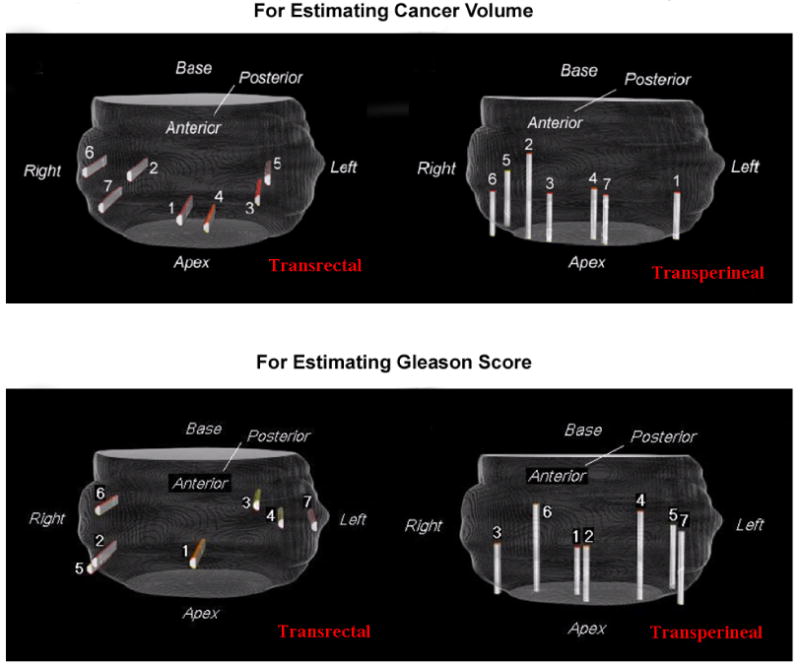
Optimized biopsy locations for estimating cancer volume (top row) and Gleason Score (bottom row), by using seven needles in both transrectal and transperineal settings.

To gain more understanding of how the optimized procedures are used to estimate, for instance, CV, we can visually superimpose the optimized transrectal procedure in the upper left part of Fig. 7 onto the statistical atlases of high and low CV specimens in the top row of Fig. 4. Then we can observe that, specimens having high CV values tend to have positive biopsies at the 1^st, 2^nd and 4^th biopsy locations, while specimens having low CV values do not. Similar observations could be drawn for estimating GS values.

All experiments were operated in C code on a 2.8 G Intel Xeon processor with UNIX operation system. In constructing the statistical atlases, it took 26 hours to normalize all 83 specimens onto the common prostate space (about 25 minutes each), which could be reduced to approximately 3 hours by paralleling the processes on 8 CPUs. Another 1.5 hours is needed for the optimization of biopsy locations and the subsequent binary classification. It is worth noting that the relatively large computational cost is not a serious problem for clinical applications, since both the statistical atlas construction and biopsy optimization are computed offline rather than real-time.

3.2. Estimation Accuracy of the Optimized Biopsy Procedures

To evaluate estimation accuracy, our optimized biopsy procedures are applied to the collected prostate specimens (the ones described in Section 2.2) with known surrogate marker values. Both leave-one-out and ten-fold cross validations are carried out. That is, we train the optimized biopsy procedures by all but one (or one-tenth) prostate specimens and test on the left-out one (or one-tenth) specimen, repeating until every specimen (or every set of one-tenth of specimens) has been left out once.

In cross validations, the estimation accuracy is measured by classification rates and the associated receiver-operating-characteristic (ROC) curves. (Recall that the estimation problem is formulated as a binary classification problem to accommodate to the clinical decisions that tend to binary). Mathematically, classification rate is the fraction of the prostate specimens that have been correctly classified/estimated in terms of high v.s. low in surrogate marker values, i.e.,

$$\text{EstimationAccuracy}=\text{ClassificationRate}=\frac{1}{N}\sum _{n=1}^{N}1\left(Z_{\text{SVM}}[f(p_n;\left\{s_1,s_2,\dots ,s_K\right\})]=C(p_n)\right)$$ (10)

where 1(X) is the logic function that equals 1 when the event X is true and 0 otherwise, Z_SVM[f] is the SVM decision function which outputs a class label (“+1” for high and “−1” for low surrogate marker value), based on the input feature vector f. In the ROC curve, the relationship between the true positive rate (TPR) and false positive rate (FPR) are plotted. TPR (also known as “sensitivity”) and FPR (also known as “1-specificity”) are defined as

$$\begin{array}{l}\text{TPR}=\frac{{\sum }_{n=1}^{N}1\left(\begin{array}{c}\left(C(p_n)=+1\right)\&\&\\ \left(Z_{\text{SVM}}\left[f(p_n;\{s_1,s_2,\dots ,s_K\})\right]=+1\right)\end{array}\right)}{{\sum }_{n=1}^{N}1(C(p_n)=+1)}\\ \text{FPR}=\frac{{\sum }_{n=1}^{N}1\left(\begin{array}{c}\left(C(p_n)=-1\right)\&\&\\ \left(Z_{\text{SVM}}\left[f(p_n;\{s_1,s_2,\dots ,s_K\})\right]=+1\right)\end{array}\right)}{{\sum }_{n=1}^{N}1(C(p_n)=-1)}.\end{array}$$ (11)

Fig. 8 shows the estimation/classification accuracy and ROC curves for the leave-one-out cross validations. The estimation/classification rates of 94.79% (or 81.93%) and the areas under ROC curve (AUC) of 0.98 (or 0.83) have been observed, when estimating CV (or GS) by 7 optimized needles in the transperineal setting. Similarly, when ten-fold cross-validation mechanism is used, the classification rates for these two cases are 92.59% and 88.75%, demonstrating a good generalization ability of our approach. More details of the estimation accuracy can be found in Table 2 for different biopsy settings in estimating different surrogate markers.

Figure 8.

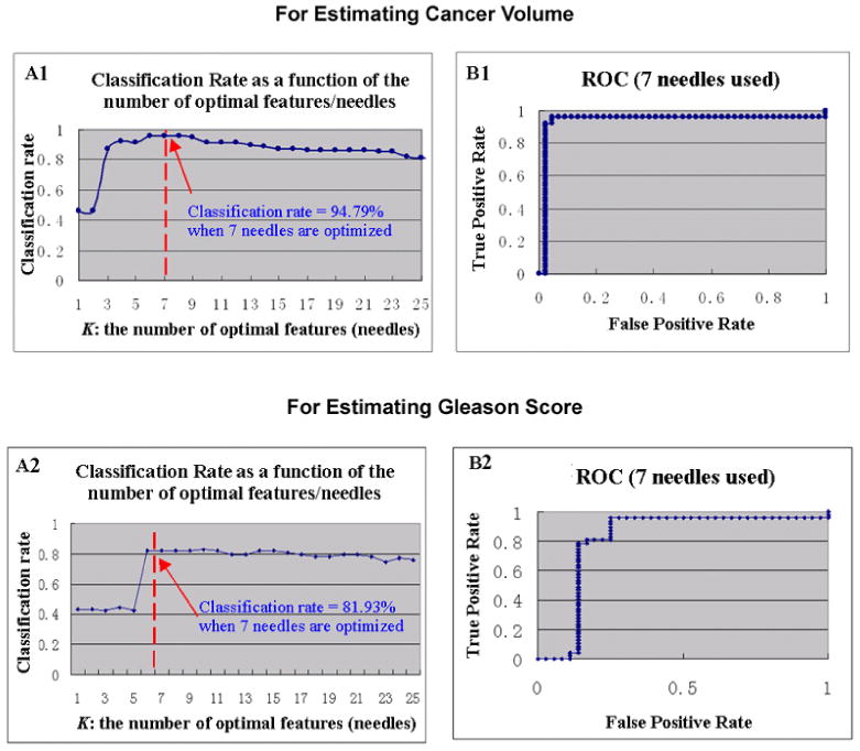
Estimation accuracy for CV (top row) and GS (bottom row), by the optimized biopsy procedures in transperineal settings. (A1&A2): classification rate as a function of the number of optimal needles. (B1&B2): ROC curve, where 7 needles were used.

Table 2.

Estimation accuracy in the leave-one-out cross validations, in terms of classification rate and the area under the ROC curve (AUC). Here, seven biopsy needles are optimized to estimate CV and GS, respectively.

	Classification Rate		AUC
	For CV	For GS	For CV	For GS
Transrectal Biopsy	93.75%	78.54%	0.96	0.79
Transperineal Biopsy	94.79%	81.93%	0.98	0.83

In Fig. 8(A1&A2), the estimation/classification accuracies are also recorded when different numbers of biopsy needles are optimized. An interesting finding is that, as long as more than 6 or 7 biopsy needles are optimized, there is no added value for additional number of biopsy needles. This finding underlines the importance of optimizing biopsy locations other than increasing the number of biopsy locations.

4. Sensitivity Analysis

Our framework is essentially an optimization problem in a population study – it optimizes biopsy locations, and the optimum is defined on the collected population of prostate specimens. Indeed, in most optimization systems or population studies like ours, a common problem is that, the performance of the system or study is usually sensitive to the variations in the optimization parameters or the input (training) populations. Those sensitive, or unstable, estimators would obviously have limited clinical use. Therefore, the question herein is, whether our framework is sensitive/unstable in these respects, and if it is, to which extent.

This section aims to evaluate the sensitivity of our framework with regard to two types of variations that can potentially limit the generalization ability of our framework: 1) variations in the optimization parameters and 2) variations in the training populations. They are described in Sections 4.1 and 4.2, respectively.

4.1. Effects of Variations in the Optimization Parameters

The effects of two major optimization parameters are examined in this section. The first major parameter is the threshold T for the Pearson's correlation coefficient. This threshold T is introduced to encourage statistical independence between any two features selected, and therefore to avoid several needles being selected around a single location. That is, in the feature ranking part (“Step 1” in Section 2.4.3), we eliminate those features that have high correlation (>correlation threshold T) with the already selected top-ranked features, before we proceed to select the next top-ranked feature. The second major parameter is the Gaussian kernel size σ for the non-linear SVM. It is introduced in SVM-based feature selection and SVM-based binary classification. Ideally, the estimation/classification accuracy of our optimized biopsy procedures should be consistent/stable, regardless of the variations in the threshold T and the SVM kernel size σ.

In our experiments, one parameter is fixed while the other varies, and the robustness of our approach is demonstrated by the consistency in the resultant estimation/classification rates and ROC curves, as shown in Fig. 9.

Figure 9.

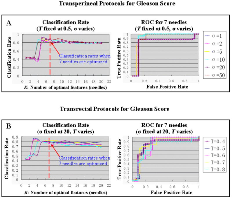
Robustness of our approach in estimating GS, with regard to the variations of two major optimization parameters (threshold T and Gaussian kernel σ). (A) T is fixed at 0.5, and σ varies from 1 to 50 (transperineal setting); (B) σ is fixed at 20, and T varies from 0.4 to 0.8 (transrectal setting).

4.2. Effects of Variations in the Training Population

In any population-based study like ours, it is understandable that different populations of subjects might yield different optimization results. The key question is to which extent.

To answer this question, we have simulated new populations of prostate specimens by a statistical simulation method known as bootstrap [11, 29]. In statistical inference, bootstrap evaluates an estimator (e.g., estimation/classification rates in our case) of the original population by simulating new populations via resampling the original population with replacement [23]. “Resampling with replacement” means that, after choosing a prostate specimen in the original population, we put it back before choosing the next specimen, until we have picked up the same number of prostate specimens as that in the original population. As a result, some prostate specimens will be selected multiple times while others not even once. For instance, if we are considering an estimator (e.g., the mean value) from an original population of natural numbers {10, 45, 20, 50, 38} and we want to establish a standard deviation for the original estimator value, we could resample the original population with replacement and thereby obtain an infinite number of simulated populations, such as {10, 20, 10, 38, 50}, {45, 20, 38, 45, 20}, and so forth. Each simulated population will yield one “simulated estimator value” and a large number (usually greater than 10 times the sample size in the original population) of such simulated estimator values will help us establish the standard deviation for the original estimator value.

Using the bootstrap method, we have simulated 850 populations, each having the same number (83) of specimens as the original population has and each leading to a cross-validated classification rate, which altogether forms a bootstrapping distribution of 850 classification rates, as shown in Fig. 10. This bootstrapping distribution reveals the mean classification rate at 87.15% and the associated standard deviation at 5.79%. Small standard variations are also found in transperineal/transrectal procedures for estimating CV/GS, prompting the robustness of our framework with regard to the variations in the training population.

Figure 10.

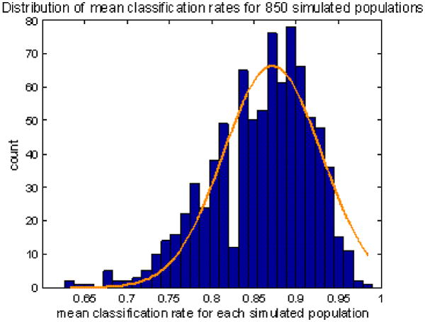
Bootstrapping distribution of the classification rates in 850 simulated populations. The mean and standard deviation is established at 87.18±5.79%, for using transperineal optimized biopsies to estimate GS. Similar results are found in transperineal / transrectal biopsy procedures when estimating CV/GS.

We chose bootstrap over Monte Carlo, another widespread simulation method because Monte Carlo simulation generates new samples from a prior knowledge of the underlying sample distribution, while bootstrap method simply re-samples the original samples without any prior knowledge of the underlying sample distribution. Bootstrap simulation method is therefore more suited in our study, since we don't have a good probabilistic cancer growth model for generating new prostate cancer specimens.

5. Discussions

In this paper, we developed optimized biopsy procedures specifically designed to estimate cancer volume (CV) and Gleason Score (GS), which are two of the most important surrogate markers for clinical significance of prostate cancer. To the best of our knowledge, our study is the first to present optimized biopsy procedures, as well as the novel estimation criterion, that can be used to specifically estimate surrogate markers for cancer significance. We have assumed and demonstrated that, by optimally sampling the spatial patterns of cancer, biopsy procedures could be used to estimate/classify whether a prostate cancer patient has high or low CV/GS values. In our framework, selecting the optimized biopsy locations is formulated as a feature selection problem, where we selected biopsy locations such that biopsy outcomes from those locations could best differentiate between specimens having different (high v.s. low) surrogate marker values. Accordingly, estimating surrogate markers is formulated as a binary classification problem, which estimates/classifies whether a new patient has high or low surrogate marker values in a way that generalizes well. Moreover, our approach is designed with the ability to account for the almost inevitable errors of needle placement in clinical practice; it is also experimentally found to be robust with regard to the major parameters in our optimization process and with regard to the input training populations.

In contrast to existing biopsy procedures, which mostly aim to improve the detection of cancer presence, our study aims to estimate surrogate markers for clinical significance of prostate cancer, which is a far more important yet far more difficult problem. For detecting cancer presence in those existing procedures, it is required that at least one biopsy needle can intersect with cancerous tissue; whereas for estimating surrogater markers, the goal in our study, it is required that the multiple biopsy needles must sample the prostate in a way that can reflect cancer spatial pattern. Because of this fundamental distinction, this paper has a completely different formulation from the existing ones. As a result, our optimized biopsy procedures can provide substantial information for the optimal treatment planning and effective cancer management.

The surrogate marker estimation in this paper is binary (high v.s. low) instead of continuously-valued, because the binary estimation better relates to the clinical decisions that tend to be binary: immediate treatment for surrogate marker values above some clinical threshold, or “watchful waiting” otherwise. Meanwhile, we have developed different biopsy procedures for estimating different surrogate markers (CV or GS). Reasons can be found in Table 1: that being high in one surrogate marker does not necessarily indicate high in the other. In occasions where CV and GS do not agree with each other (in terms of high v.s. low), how to utilize the estimated CV and GS values to evaluate clinical significance of prostate cancer becomes a quite challenging problem. Actually, other than CV and GS, there are numerous other surrogate markers that will also contribute to the determination of the clinical significance of prostate cancer. Such surrogate markers include, but are not limited to, age, genetic factors and ethnic factors. Kibel stated in [27]: “The 40-year-old patient with a 0.5 cc tumor is of much greater concern than the 80-year-old with a 1.0 cc tumor.” Till recently, how to comprehensively use all those surrogate markers to conclude the cancer significance is still a challenging problem under debate [3, 43]. Therefore, this paper only discusses estimations of surrogate markers CV and GS, and the further evaluation of cancer significance goes beyond the scope of this paper.

Our study has yielded several interesting observations. Firstly, we have observed in Fig. 8(A1&A2) that the increased number of biopsy needles over 6 or 7 does not provide added estimative value, and should rather be avoided because of the marginal decrease in estimation accuracy and the increase in patient pain as well as the associated morbidities. This provides quantitative reference for the ongoing debate about how many needles are appropriate to balance between patient pain and the detection of clinically-significant prostate cancers. Secondly, we have observed qualitatively in Fig. 8 and quantitatively in Table 2 that, the estimation accuracy for cancer volume is noticeably higher than that for Gleason Score. A plausible explanation could be that cancer volume is a quantity that is more closely correlated to the spatial pattern of prostate cancer and could therefore be better sampled and estimated by the optimally-placed biopsy needles. Generally, larger cancers are expected to have grown closer to the capsule boundary than smaller cancers; therefore needles placed in those locations would be more likely to determine whether a tumor is large or small with high accuracy. This prompts future investigations, especially from the clinical perspective, of the correlations between cancer spatial patterns and cancer surrogate markers.

The presented framework is general. It could thereby be readily applied to different populations, different surrogate markers, different types of human cancer and even different clinical procedures other than biopsy. For example, our framework could be potentially used to find whether different patient groups (stratified by ethnicity, age or PSA level) tend to develop clinically-significant prostate cancers at different locations on statistical basis. Additionally, it could also be used to guide focal radiotherapy or other spatially-confined treatments to those locations that are statistically more likely to develop clinically-significant prostate cancer, thus increasing the treatment efficiency.

A potential limitation of our study is the relatively small sample size: 83 prostate specimens might not be sufficient to accurately represent cancer distributions in the entire population of prostate cancer patients. Actually, this limitation is inherent to any approach attempting to derive cancer distribution (e.g., [45, 42, 49, 34]). A possible solution would be to encourage multi-institutional studies and data sharing processes, so that larger sample size could be independently acquired and the “true” cancer distribution could be approximated with less bias. Meanwhile, we are planning to validate our optimized biopsy procedures in new groups of patients, initially via ex vivo biopsy of the surgically extracted prostatectomy specimens.

In summary, we have presented an approach to derive optimized biopsy procedures, for estimating cancer volume and Gleason Score, two of the most important surrogate markers for clinical significance of prostate cancer. More validations and inter-institutional collaborations are expected in the future.

References

- 1.Cancer Facts and Figures. Atlanta: American Cancer Society; 2008. http://www.cancer.org. [Google Scholar]
- 2.Akin O, Hricak H. Imaging of prostate cancer. Radiol Clin North Am. 2007;45:207–222. doi: 10.1016/j.rcl.2006.10.008. [DOI] [PubMed] [Google Scholar]
- 3.Albertsen P. Defining clinically significant prostate cancer: pathologic criteria versus outcomes data. Journal of the National Cancer Institute. 1996;88:1177–1178. doi: 10.1093/jnci/88.17.1177. [DOI] [PubMed] [Google Scholar]
- 4.Brown MPS, et al. Knowledge-based analysis of microarray gene expression data by using support vector machines. Proceedings of National Academy of Science (PNAS) 2000;97:262–267. doi: 10.1073/pnas.97.1.262. [DOI] [PMC free article] [PubMed] [Google Scholar]
- 5.Burges C. A tutorial on support vector machines for pattern recognition. Data Mining and Knowledge Discovery. 1998;2:121–167. [Google Scholar]
- 6.Cai H, et al. Probabilistic Segmentation of Brain Tumors on Multi-modality Magnetic Resonance Images. IEEE International Symposium on Biomedical Imaging; Washing D.C., USA: 2007. [Google Scholar]
- 7.Chen ME, et al. Optimization of Prostate Biopsy Strategy Using Computer Based Analysis. The Journal of Urology. 1997;158:2168–2175. doi: 10.1016/s0022-5347(01)68188-6. [DOI] [PubMed] [Google Scholar]
- 8.Cookson MS, et al. Correlation between Gleason Score of Needle Biopsy and Radical Prostatectomy Specimen: Accuracy and Clinical Implications. J of Urology. 1997;157(2):559–562. [PubMed] [Google Scholar]
- 9.De Craene M, et al. Multi-subject Registration for Unbiased Statistical Atlas Construction. MICCAI. 2004:655–662. [Google Scholar]
- 10.Desouza N, et al. Magnetic resonance imaging in prostate cancer: value of apparent diffusion coefficients for identifying malignant nodules. British Journal of Radiology. 2007;80:90–95. doi: 10.1259/bjr/24232319. [DOI] [PubMed] [Google Scholar]
- 11.Efron B, Tibshirani R. Bootstrap Methods for Standard Errors, Confidence Intervals, and Other Measures of Statistical Accuracy. Statistical Science. 1986;1:54–75. [Google Scholar]
- 12.Epstein J, et al. Use of Repeat Sextant and Transition Zone Biopsies for assessing extent of prostate cancer. Journal of Urology. 1997;158:1886–1890. doi: 10.1016/s0022-5347(01)64159-4. [DOI] [PubMed] [Google Scholar]
- 13.Fan Y, et al. COMPARE: Classification of Morphological Patterns Using Adaptive Regional Elements. IEEE Transactions on Medical Imaging. 2007;26:93–105. doi: 10.1109/TMI.2006.886812. [DOI] [PubMed] [Google Scholar]
- 14.Fink K, et al. Prostate cancer detection with two sets of ten-core sextant biopsies. Urology. 2001;58:735–9. doi: 10.1016/s0090-4295(01)01352-8. [DOI] [PubMed] [Google Scholar]
- 15.Frangi AF, et al. Automatic construction of multiple-object three-dimensional statistical shape models: application to cardiac modeling. IEEE Trans on Med Im. 2002;21(9):1151–1166. doi: 10.1109/TMI.2002.804426. [DOI] [PubMed] [Google Scholar]
- 16.Freund Y, Schapire R. A Short Introduction to Boosting. Journal of Japanese Society for Artificial Intelligence. 1999;14:771–780. [Google Scholar]
- 17.Furey TS, et al. Support vector machine classification and validation of cancer tissue samples using microarray expression data. Bioinformatics. 2000;16:906–914. doi: 10.1093/bioinformatics/16.10.906. [DOI] [PubMed] [Google Scholar]
- 18.Futterer JJ, et al. Staging Prostate Cancer with Dynamic Contrast-enhanced Endorectal MR Imaging prior to Radical Prostatectomy: Experienced versus Less Experienced Readers. Radiology. 2005;237:541–549. doi: 10.1148/radiol.2372041724. [DOI] [PubMed] [Google Scholar]
- 19.Gleason DF. The Veteran's Administration Cooperative Urologic Research Group: histologic grading and clinical staging of prostatic carcinoma. In: Tannenbaum M, editor. Urologic Pathology: The Prostate. Lea and Febiger; Philadelphia: 1977. pp. 171–198. [Google Scholar]
- 20.Guyon I, Elisseeff A. An introduction to variable and feature selection. Journal of machine learning research. 2003;3:1157–1182. [Google Scholar]
- 21.Guyon I, et al. Gene Selection for Cancer Classification using Support Vector Machines. Machine Learning. 2002;46:389–422. [Google Scholar]
- 22.Hautmann S, et al. Detection rate of histologically insignificant prostate cancer with systematic sextant biopsies and fine needle aspiration cytology. Journal of Urology. 2000;163:1734–1738. [PubMed] [Google Scholar]
- 23.Hesterberg T, et al. Bootstrap Methods and Permutation Tests. Second. W. H. Freeman; New York: 2005. [Google Scholar]
- 24.Hodge K, et al. Random Systematic Versus Directed Ultrasound Guided Transrectal Core Biopsies of the Prostate. Journal of Urology. 1989;142:71. doi: 10.1016/s0022-5347(17)38664-0. [DOI] [PubMed] [Google Scholar]
- 25.Hricak H, et al. Imaging prostate cancer: a multidisciplinary perspective. Radiology. 2007;243(1):28–53. doi: 10.1148/radiol.2431030580. [DOI] [PubMed] [Google Scholar]
- 26.Johnstone PA, et al. ‘Insignificant’ prostate cancer on biopsy: pathologic results from subsequent radical prostatectomy. Prostate Cancer Prostatic Dis. 2007;10(3):237–41. doi: 10.1038/sj.pcan.4500963. [DOI] [PubMed] [Google Scholar]
- 27.Kibel AS. Optimizing Prostate Biopsy Techniques. Journal of Urology. 2007;177:1976–1977. doi: 10.1016/j.juro.2007.03.073. [DOI] [PubMed] [Google Scholar]
- 28.Kirkham A, et al. How good is MRI at detecting and characterising cancer within the prostate? Eur Urol. 2006;50:1163–1174. doi: 10.1016/j.eururo.2006.06.025. [DOI] [PubMed] [Google Scholar]
- 29.Manly B. Randomization, Bootstrap and Monte Carlo Methods in Biology. 3 Chapman & Hall/CRC; 2006. [Google Scholar]
- 30.Manseck A, et al. Is systematic sextant biopsy suitable for the detection of clinically significant prostate cancer? Urologia Internationalis. 2000:80–83. doi: 10.1159/000064844. [DOI] [PubMed] [Google Scholar]
- 31.Narain V, et al. How accurately does prostate biopsy Gleason score predict pathologic findings and disease free survival? The Prostate. 2001;49(3):185–190. doi: 10.1002/pros.1133. [DOI] [PubMed] [Google Scholar]
- 32.Osuna E, et al. Training Support Vector Machines: an Application to Face Detection. IEEE Computer Society Conference on Computer Vision and Pattern Recognition (CVPR'97).1997. [Google Scholar]
- 33.Ou Y, et al. Cascaded segmentation of brain tumors using multi-modality MR profiles. ISMRM; Berlin, Germany: 2007. [Google Scholar]
- 34.Ou Y, et al. MICCAI 2008. Prostate Image Workshop; New York: 2008. Sept, Optimized Biopsy Procedures for Estimating Gleason Score and Prostate Cancer Volume. 2008. [DOI] [PMC free article] [PubMed] [Google Scholar]
- 35.Ou Y, Davatzikos C. DRAMMS: Deformable Registration via Attribute Matching and Mutual-Saliency weighting. Information Processing in Medical Imaging (IPMI); Williamsburg, Virginia: 2009. Jul, 2009. [DOI] [PubMed] [Google Scholar]
- 36.Ou Y, et al. Computer Vision and Pattern Recognition Workshop (CVPRW) Mathematical Methods in Biomedical Image Analysis (MMBIA); Miami: 2009. Non-Rigid Registration between Histological and MR Images of the Prostate: A Joint Segmentation and Registration Framework. 2009. [Google Scholar]
- 37.Park H, et al. Construction of an abdominal probabilistic atlas and its application in segmentation. IEEE TMI. 2003;22(4):483–492. doi: 10.1109/TMI.2003.809139. [DOI] [PubMed] [Google Scholar]
- 38.Quinlan J. Induction of Decision Trees. Machine Learning. 1986;1:81–106. [Google Scholar]
- 39.Rakotomamonjy A. Variable Selection Using SVM-based Criteria Journal of Machine Learning Research. 2003;3:1357–1370. [Google Scholar]
- 40.Sebo TJ, et al. The percent of cores positive for cancer in prostate needle biopsy specimens is strongly predictive of tumor stage and volume at radical prostatectomy. J of Urology. 2000;163(1):174–178. [PubMed] [Google Scholar]
- 41.Shen D, et al. An adaptive focus statistical shape model for segmentation and shape modeling of 3D brain structures. IEEE Transactions on Medical Imaging. 2001;20:257–271. doi: 10.1109/42.921475. [DOI] [PubMed] [Google Scholar]
- 42.Shen D, et al. Optimized Biopsy Strategy by A Statistical Atlas of Prostate Cancer Distribution. Med Im Anal. 2004;8(2):139–150. doi: 10.1016/j.media.2003.11.002. [DOI] [PubMed] [Google Scholar]
- 43.Singh H, et al. Improved Detection of Clinically Significant, Curable Prostate Cancer With Systematic 12-Core Biopsy. The Journal of Urology. 2004;171:1089–1092. doi: 10.1097/01.ju.0000112763.74119.d4. [DOI] [PubMed] [Google Scholar]
- 44.Siu W, et al. Use of extended pattern technique for initial prostate biopsy. Journal of Urology. 2005;174:505–509. doi: 10.1097/01.ju.0000165385.53652.7a. [DOI] [PubMed] [Google Scholar]
- 45.Sofer A, et al. Optimal Biopsy Protocols for Prostate Cancer. Annals of Operations Research. 2003;119:63–74. [Google Scholar]
- 46.Stamatiou K, et al. Impact of additional sampling in the TRUS-guided biopsy for the diagnosis of prostate cancer. Urol Int. 2007;78:313–317. doi: 10.1159/000100834. [DOI] [PubMed] [Google Scholar]
- 47.Verma R, et al. Multiparametric Tissue Characterization of Brain Neoplasms and Their Recurrence Using Pattern Classification of MR Images. Academic Radiology. 2008;15:966–977. doi: 10.1016/j.acra.2008.01.029. [DOI] [PMC free article] [PubMed] [Google Scholar]
- 48.Zhan Y, Shen D. Deformable segmentation of 3D ultrasound prostate images using statistical texture matching method. IEEE Trans Med Imag. 2006 Mar;25(no 3):256–273. doi: 10.1109/TMI.2005.862744. 2006. [DOI] [PubMed] [Google Scholar]
- 49.Zhan Y, et al. Targeted Prostate Biopsy Using Statistical Image Analysis. IEEE Transactions on Medical Imaging. 2007;26:779–788. doi: 10.1109/TMI.2006.891497. [DOI] [PubMed] [Google Scholar]
- 50.Zhan Y, et al. Registering Histological and MR Images of Prostate for Image-based Cancer Detection. Acad Radiol. 2007;14(11):1367–1381. doi: 10.1016/j.acra.2007.07.018. [DOI] [PMC free article] [PubMed] [Google Scholar]
- 51.Zhao W, et al. Discriminant analysis of principal components for face recognition. Proceedings. Third IEEE International Conference on Automatic Face and Gesture Recognition.1998. [Google Scholar]