Multimodal and Multi-tissue Measures of Connectivity Revealed by Joint Independent Component Analysis

Abstract

The human brain functions as an efficient system where signals arising from gray matter are transported via white matter tracts to other regions of the brain to facilitate human behavior. However, with a few exceptions, functional and structural neuroimaging data are typically optimized to maximize the quantification of signals arising from a single source. For example, functional magnetic resonance imaging (FMRI) is typically used as an index of gray matter functioning whereas diffusion tensor imaging (DTI) is typically used to determine white matter properties. While it is likely that these signals arising from different tissue sources contain complementary information, the signal processing algorithms necessary for the fusion of neuroimaging data across imaging modalities are still in a nascent stage. In the current paper we present a data-driven method for combining measures of functional connectivity arising from gray matter sources (FMRI resting state data) with different measures of white matter connectivity (DTI). Specifically, a joint independent component analysis (J-ICA) was used to combine these measures of functional connectivity following intensive signal processing and feature extraction within each of the individual modalities. Our results indicate that one of the most predominantly used measures of functional connectivity (activity in the default mode network) is highly dependent on the integrity of white matter connections between the two hemispheres (corpus callosum) and within the cingulate bundles. Importantly, the discovery of this complex relationship of connectivity was entirely facilitated by the signal processing and fusion techniques presented herein and could not have been revealed through separate analyses of both data types as is typically performed in the majority of neuroimaging experiments. We conclude by discussing future applications of this technique to other areas of neuroimaging and examining potential limitations of the methods.

I. Introduction

There has been an increasing appreciation that distributed neural circuits, comprised of gray matter regions linked together by white matter tracts, are the mechanism by which the brain supports basic sensory processes and even higher cognitive function [1]. Recent advances in neuroimaging technologies have vastly increased the scientific community’s ability to non-invasively measure both brain structure and function. Specifically, neuroimaging techniques such as functional magnetic resonance imaging (FMRI), magnetoencephalography (MEG), electroencephalography (EEG), diffusion tensor imaging (DTI) and structural magnetic resonance imaging (MRI) each provide information about different underlying signals (e.g., electrophysiological versus hemodynamic) from different tissue types (e.g., neurons in gray matter versus axons in white matter) that have different spatial and temporal properties as well as different signal and noise characteristics. This plethora of information results in unique challenges in signal processing for each imaging modality, which become even more complex when information is combined across different modalities. In the current application, we focus on using standard signal processing techniques and novel multi-variate analytic techniques to combine two measures of functional connectivity derived from both white matter (DTI) and gray matter (resting state FMRI) data (see Fig. 1). Detailed descriptions of white and gray matter connectivity in addition to potential methods for combining these measurements are now presented.

Fig. 1.

A cartoon figure of two common measures of gray and white matter connectivity. The areas in the gray matter (yellow coloring) correspond to the 1) anterior and 2) posterior cingulate gyrus, which are two of the key components of the default mode network (DMN). Fractional anisotropy values for the white matter tracts are also presented. Individual tracts are color-coded for the primary direction of axonal orientation according to left-right axis (L-R; red), posterior-anterior axis (P-A; green) or inferior-superior axis (I-S; blue).

A. Measures of White Matter Connectivity

One of the unique features of the human brain is the relatively high conduction velocity between neurons facilitated by myelinated axons [2]. The link between white matter integrity and cognitive functioning has been demonstrated in research linking cognitive development to increased myelination over time in children [3], as well as decreased myelination associated with age-related cognitive decline [4]. To date, the most effective method of measuring the different properties of white matter is DTI [5;6]. The primary signal source in DTI arises from the different diffusion rates of water molecules secondary to Brownian motion in different neuronal structures [5;6]. Diffusion in white matter is relatively anisotropic because the water molecules move more freely along the path of the axon, but are restricted transversally by the axon cell walls. In contrast, diffusion is both greater and more isotropic in ventricles containing cerebral spinal fluid due to the lack of a constraining structure. Within white matter, the diffusion of water molecules is also dependent on the density and integrity of the myelin, the number of axonal tracks bundled together along similar pathways and the permeability of the local membranes [5;7]. These structural variations in white matter can be quantified with DTI [7;8] through the calculated value of fractional anisotropy (FA), mean diffusivity (MD) radial diffusivity (RD), and axial diffusivity (AD).

The diffusion tensor is a 3×3 positive semi-definite symmetric matrix D, describing the random translational motion of water molecules in three dimensions [9]. The diffusion tensor can be measured by a Stejskal-Tanner [10] experiment done in multiple directions. The MRI signal intensity at a voxel is given by

$$S=S_0{e}^{-{bg}^{T}Dg},$$ (1)

where b is the diffusion sensitizing parameter that depends on gradient strength, gradient duration, and the time between the two bipolar gradient pulses, g is a unit vector along the gradient direction, and S₀ is the image intensity for b=0. D, being a symmetric matrix, has 6 unknowns and combined with S₀ there are 7 unknowns. Thus with 7 diffusion experiments, one with b=0 and six others for independent gradient directions (g), we can calculate D. The tensor can be diagonalized to obtain three eigenvalues (λ₁, λ₂, λ₃), in descending order, with λ₁ being the largest, and the three corresponding orthonormal eigenvectors (e₁,e₂,e₃). The eigenvector e₁, corresponding to eigenvalue λ₁, is called the principal eigenvector.

To relate the properties of the diffusion tensor to more meaningful physical concepts alternative scalar measures are defined. These measures have been chosen to capture the two-dimensional diffusion in axon bundles, which for simplicity can be considered to be a collection of narrow tubes with preferential diffusion in one direction. Mean diffusivity (MD) is defined by

$$MD=\lambda =({\lambda }_1+{\lambda }_1+{\lambda }_1)/3.$$ (2)

The axial (AD) and radial (RD) diffusivities are respectively defined by

$$AD={\lambda }_1$$ (3)

and

$$RD=({\lambda }_2+{\lambda }_3)/2.$$ (4)

The axial diffusivity is a measure of the diffusivity along the axon bundle since this is the preferential direction for diffusion. The diffusion in the plane perpendicular to the axons has no special preference and radial diffusivity is defined to characterize it. Fractional anisotropy is defined by

$$FA=\frac{\sqrt{3}}{\sqrt{2}}·\frac{\sqrt{{({\lambda }_1-\lambda )}^2+{({\lambda }_2-\lambda )}^2+{({\lambda }_3-\lambda )}^2}}{\sqrt{{\lambda }_1^2+{\lambda }_2^2+{\lambda }_3^2}},$$ (5)

where FA is a measure of diffusion anisotropy and is in the range of (0,1). If the diffusion is isotropic, FA = 0, and if the diffusion is completely in one direction then FA = 1.

FA has served as the most widely used marker of white matter connectivity and integrity in the literature to date. A lower FA is associated with poorer organization of fiber bundles as FA decreases when diffusion becomes more isotropic due to a lack of white matter integrity. However, decreased FA values can result from either a decrease in AD or an increase in RD which in turn can be caused by two different physical mechanisms. Specifically, a decrease in AD (and associated reduction in FA) can be caused by axonal damage. An increase in RD (and associated reduction in FA) can result from a breakdown of the myelin sheath surrounding the axons, resulting in greater mobility of water molecules diffusing radially away from the axons [11]. Therefore, if differences in FA in white matter are observed, analyzing AD and RD will provide better insight about the cause of FA change. Although DTI has conventionally been used to measure white matter properties, information is also present for gray matter structure. At the current resolution of most imaging protocols, diffusion is observed to be isotropic in gray matter (small FA and greater MD). Therefore, AD and RD do not provide unique information and gray matter diffusion may be more appropriately characterized by MD.

B. Measures of Gray Matter Connectivity

FMRI was developed in the early 1990’s [12;13] based on the different paramagnetic properties of deoxyhemoglobin, cerebral blood flow and cerebral blood volume that occur following neuronal activity and has become the most-widely used neuroimaging technique [14]. In a typical FMRI experiment, a sensory or cognitive task is performed and the subsequent data is modeled using general linear model (GLM) statistics such as multiple regression [15] or deconvolution [16]. The GLM often assumes that the time series are independent and identically distributed (i.i.d.) and that the variance is constant across all voxels [17]. However, a major limitation of GLM is that it is only capable of distinguishing regions of the brain that show a relationship with a predetermined hemodynamic response of the stimuli. Specifically, the most basic GLM (the student t-test) used to determine brain activity is given by

$$t_0=\frac{{\mu }_B-{\mu }_A}{\sqrt{{\widehat{\sigma }}^2(1/T_A+1/T_B)}},$$ (6)

where μ_A and μ_B are the sample means of the time series when stimuli A and stimuli B (or a baseline period) are being delivered. T_A and T_B are the amounts of time that conditions A or B take place. σ̂² is an estimate of the common variance given by

$${\widehat{\sigma }}^2=\frac{(T_A-1)s_A^2+(T_B-1)s_B^2}{(T_A+T_B-2)},$$ (7)

with $s_A^2=1/(T_A-1){\sum }_{t\in A}{(x(t)-{\mu }_A)}^2$ where x(t) is the hemodynamic response over time. This basic GLM framework can be expanded into a regression equation which not only accounts for experimental manipulations, but also for constants and first or second order polynomials.

Data-driven techniques, such as independent component analysis (ICA), have more recently been applied to FMRI data to discover underlying brain activity [18;19]. ICA is a statistical and computational technique used for revealing hidden factors that underlie sets of random variables, signals or measurements and performs a blind-source separation of overlapping signals into individual spatial and temporal components [20]. The ICA of a random vector consists of a linear transformation that minimizes the statistical dependence between the components. It can be viewed as an extension of principal component analysis (PCA), which only imposes independence up to the second order with an additional orthogonality constraint. The key assumption in ICA is that the sources are statistically independent, and although this is probably not strictly true for FMRI signals, the algorithm has been proven to be robust [19]. Another requirement is that, to perform a unique separation of the sources, no more than one of the signals of interest can have a Gaussian probability distribution function.

The ICA model is described by x = As, where s is the source defined by an M-dimensional random vector, A_{(V x M)} is the unknown mixing matrix and x is the observed signal denoted by a V-dimensional random vector. M is the number of sources and V is the number of voxels. The length of the vectors of x and s is T (number of time steps). Usually M is greater or equal to V, so A is typically of full rank. In addition, in the preprocessing steps of ICA, the data in x is whitened (mean removed and variance set to 1) so that the scale of the data will be removed for all subsequent calculations. The goal of the ICA algorithm is to estimate W_{(M x V)} such that ŝ = Wx, where W is the estimated unmixing matrix and is the approximation of the sources. There have been a variety of algorithms created to calculate the W matrix, including Infomax [21], FastICA [22], joint approximate diagonalization of eigenmatrices (JADE) [20], simultaneous blind extraction using cumulants (SIMBEC) [23], and AMUSE [24]. However, research indicates that Infomax is a good choice for FMRI data due to its consistency, reliability, noise reduction capabilities and ability to yield results with the highest t-values compared to several other approaches [25]. Infomax finds the independent components by maximization of the joint output entropy of sources passed through a non-linear squashing function [26]. This approach updates the weights through an iterative equation using gradient ascent

$$W_i=W_{i-1}+\mathrm{\Delta }W.$$ (8)

The update is given by: ΔW = −η[I + ϕ(u)u^H]W, where ϕ(u) = 2tanh(u) and the non-linearity is chosen as tanh(u). This approach has been shown to be equivalent to a maximum likelihood method when the derivative of the non-linearity matches the assumed source density [21].

This algorithm can be extended to apply to neuroimaging data derived from a group of subjects [27]. In Group ICA, instead of having one set of components for each subject, one set of “group” components is estimated from the full data set. Entering all the subjects into an ICA analysis has an advantage that this method orders the components of different subjects the same way. It is computationally heavy to estimate components of whole brain data sets for a group of subjects; therefore data-reduction methods are performed prior to the ICA. Specifically, the data from individual subjects are first reduced in dimension using PCA decomposition [28] and are then concatenated together to form one large dataset, which is further reduced using PCA decomposition on a group level (prior to the ICA estimation). An aggregate unmixing matrix (W^G) is created and can be defined as

$$W^G=\left[\begin{array}{llll}{W}_1\hfill & W_2\hfill & \dots \hfill & W_I\hfill \end{array}\right],$$ (9)

where W₁ … W_I are the individual unmixing matrices corresponding to the subject’s partition and I is the number of subjects. This is possible due to the heuristics adopted in the group ICA algorithm [27]. Thus, the individual unmixing matrices can be considered separable and hypothesis tests can be performed by fitting the individual subject timecourses to a GLM model [29]. It is also possible to perform back-reconstruction to calculate individual subject component images.

The application of ICA has been especially important for FMRI studies of functional connectivity during the collection of resting state data [30]. Because ICA is a data-driven approach, it permits the identification of networks of brain regions that synchronously fluctuate either at rest or during a task. Moreover, unlike GLM analyses, it is not constrained by a priori models specifying when and where the resultant activation is expected to occur. Functional regions that exhibit similar fluctuations in signal are grouped into different components that represent different networks of correlated activity. Although several networks (i.e., components) have been identified during the collection of resting state data [31], the most widely discussed component corresponds to the default mode network (DMN). The DMN has been previously defined during studies of resting glucose metabolism [32] and decreased activation following mental activity during both PET [33;34], FMRI [35], and EEG [36]. The most commonly reported regions [31;33;37–40] of the human brain that compose the DMN (see Fig. 2) include the posterior cingulate gyrus (Brodmann’s areas (BA) 23,31), posterior parietal lobule (BA 7,39,40), dorsolateral and superior frontal areas (BA 8,9,10), and anterior cingulate gyrus (BA 11, 32). Although the exact function of the DMN remains unknown, some researchers have suggested that it corresponds to the baseline state of passive mental activity associated with random episodic thought processes [30;41–43]. The interested reader is referred to an excellent review paper on DMN structures and potential functionality [30].

Fig. 2.

Representation of the default mode network depicting the major nodes of the network including the anterior and posterior cingulate gyrus, inferior and superior parietal lobes and superior frontal gyrus. Axial slice locations (Z) are presented according to the origin in Talairach space and the two hemispheres are labeled for right (R) and left (L). The intensity values of the mask were obtained by first creating a binary mask of regions previously reported to be active in the default mode literature and then smoothing with a 10 mm Gaussian FWHM filter. Intensity values are color-coded and range from 0 to 1 dependent on the spatial proximity to stereotaxically defined default mode nodes of activation.

C. Potential Methods for Combining Connectivity Measures

Currently, joint ICA (J-ICA) is one of the few existing multivariate methods that are capable of fusing information from two or more imaging modalities and identifying regions (possibly different regions in the two modalities) that are coupled together [44;45]. Other existing tools for examining joint information across multiple imaging modalities include region-based approaches such as structural equation modeling or dynamic causal modeling [46]. However, these approaches do not provide an examination of all available information (i.e., the full set of brain voxels), which is one of the proposed benefits of both FMRI and DTI. Methods that transform data matrices into a smaller set of modes or components, such as singular value decomposition [47;48] and ICA, are also alternative methods for data fusion. However, J-ICA technique provides several advantages compared to these other data fusion techniques. Foremost, the use of a feature-based approach provides a mechanism for examining data that was modeled at the first level following the signal processing steps that are unique to each imaging modality. Therefore, it is less dependent on individual and somewhat arbitrary decisions such as solving of the inverse problem (MEG/EEG) or the selection of a statistical parametric threshold (FMRI data). Second, J-ICA enables the analysis of different types of data in a unified analytic framework. Third, J-ICA does not preferentially treat the information from either imaging modality, such as occurs when data from one modality are used as priors [49]. Finally, this approach also separates the data into joint components, each of which has a DTI and an FMRI portion, which may be especially useful for applications in clinical neuroscience (e.g., component-specific differences in different patient groups). Most importantly, these features can then be queried for shared dependence, which is not detectable with a simple voxel-wise subtractive or conjunctive approach. Herein lies the true benefit of J-ICA, as the resultant maps do not merely represent areas that have separately been identified by the individual imaging techniques (i.e., conjunction), but rather signals of two distinct modalities are used to inform one another.

In J-ICA each data type (e.g., FMRI or DTI) is first reduced to a feature. Similar to the traditional ICA formulation, for each modality J-ICA is defined by x = A_k s_k where s_k the source defined by a M-dimensional vector source, A_{k (V x M)} is the unknown mixing matrix and x_k is the observed signal defined by a V-dimensional vector, where k is the modality, M is number of sources and V is the number of voxels. The vector x is of size I, where I is the number of subjects. Next, new variables composed from the two modalities are defined $x_{(Ix2V)}^J=[x_1\mid x_2]$ and $s_{(Mx2V)}^J=[s_1\mid s_2]$. The result is the new shared mixing matrix, x^J = A^J s^J, where A^J is of size I by M. Similar to ICA, the J-ICA algorithm has to estimate an unmixing matrix W^J_{(M x I)} such that ŝ^J =W^J x^J, where ŝ^J_{(M x 2V)} is the approximation of the two sources. Therefore, s ^^J contains the joint components of the two modalities. The Infomax algorithm can then also be used to obtain the W^J unmixing matrix similar to methodology described above.

To date, we are unaware of a study that has examined the shared variance associated with measures of both gray (resting state FMRI with the use of ICA) and white (DTI) matter connectivity in the same subject population on a voxel-wise level. Although J-ICA has been performed on structural [44] and EEG [50] data and DTI with patient population [45] with FMRI it has never been done for these two measures of connectivity using a purely data driven approach, where the DMN is revealed using ICA. Even though resting state FMRI and DTI have been independently used to quantify neuronal connectivity, it is likely that combining the information from these two imaging modalities will provide new and unique information about functional connectivity. Therefore, four separate J-ICA analyses were conducted between the DMN component identified from the resting state FMRI data and the 4 scalars (FA, MD, RD and AD) commonly calculated during the analyses of DTI data. Our overall hypothesis was that white matter density (FA) and axonal integrity (AD) would be directly associated with the robustness of activity in the DMN during resting state. We further predicted that the corpus callosum, which is the primary fiber bundle that mediates communication between the two hemispheres, would demonstrate the strongest relationship between DTI and FMRI measures.

II. Methods

A. Subjects

Twenty-four (12 males, 12 females) right-handed (mean Edinburgh Handedness Inventory score = 75.50% +/−23.94%) adult volunteers (mean age = 25.16+/−4.72) completed the study. None of the study participants were taking psychoactive medications or had a history of neurological, psychiatric or substance abuse disorders. Informed consent was obtained from all subjects according to institutional guidelines at the University of New Mexico.

B. Data Acquisition Task

All data was collected on a Siemens 1.5 Tesla scanner using an eight-channel radio-frequency coil (RF) and using SENSE. Subjects rested supine in the scanner with their head secured by chin and forehead straps, with additional foam padding to limit head motion within the head coil. At the beginning of the scanning session, a single, high resolution T1 [TE (echo time) = 4.76 ms, TR (repetition time) = 12 ms, 20° flip angle, number of excitations (NEX) = 1, slice thickness = 1.5 mm, FOV (field of view) = 256 mm, resolution = 256 × 256] anatomic image was collected. A total of three different resting state runs were collected for each subject. During each run, 90 echo-planar images were acquired using a single-shot, gradient-echo echoplanar pulse sequence [TR = 2000 ms; TE = 36 ms; flip angle = 90°; FOV = 256 mm; matrix size = 64 × 64]. Twenty-eight contiguous, sagittal 5.5-mm thick slices were selected to provide whole-brain coverage (voxel size: 4 × 4 × 5.5 mm). The first two images of each run were subsequently eliminated to account for T1 equilibrium effects, leaving a total of 88 images per run.

Two or three DTI scans were acquired for each subject along the AC-PC line using a single-shot spin echo, echo planar imaging sequence with 6 diffusion gradients [TE = 70 ms; TR = 8500 ms; FOV = 256 × 256 mm; matrix size = 128 × 128]. The twice-refocused spin echo sequence was chosen for data acquisition to reduce the effects of eddy currents secondary to gradient switching, to reduce artifacts associated with head movement and allow increased time for diffusion sensitizing gradients [51]. Generalized autocalibrating partially parallel acquisitions (GRAPPA) with 2× acceleration was also used to reduce susceptibility-induced image distortions [52]. A total of 74 contiguous axial slices were collected for whole brain coverage with a slice thickness of 2 mm, resulting in a voxel resolution of 2 mm³.

Presentation software (Neurobehavioral Systems) was used for stimulus presentation and synchronization of stimulus events with the MRI scanner during the resting state task. Visual stimuli were rear-projected using a Sharp XG-C50X LCD projector on an opaque white Plexiglas projection screen. Subjects were asked to relax and passively stare at a fixation cross (visual angle = 1.54°) for three minutes (90 images) with their eyes open during the three separate runs. Although research suggests that the resulting patterns of brain activity are similar for paradigms in which subjects keep their eyes opened or closed [33;38], subjects were requested to keep their eyes open to minimize the likelihood that they would fall asleep and to avoid the electrophysiological spectrum changes (i.e., increased alpha waves) associated with closed eyes [36]. Subjects were requested to keep head movement to a minimum throughout the functional imaging, DTI and anatomical scans.

C. Data Analyses

All data were analyzed in a hierarchical fashion. Specifically, data from the individual modalities (resting state FMRI and DTI) were first pre-processed to improve signal-to-noise characteristics and to meet the assumptions necessary for the level-one analyses. For the resting FMRI data, ICA and Group ICA were performed as level-one analyses to identify the appropriate feature (i.e., DMN activity) of interest. For the DTI data, level-one analyses consisted of the calculation of the eigenvectors and eigenvalues so that the appropriate scalar values (i.e., FA, MD, RD and AD) could be determined. The individual features from these two level-one analyses were then analyzed for shared variance using four separate J-ICAs. An outline of the pre-processing through level-two analyses can be seen in Fig. 3. The individual steps involved in these data analyses are now discussed in more detail.

Fig. 3.

Processing pipeline used to perform the joint analysis of the resting state FMRI (default mode network component) and the DTI (FA, MD, AD, RD) data. A detailed description of each block is described in the methods section.

D. FMRI Processing

Functional images were generated and processed using a mixture of freeware and commercial packages including the Analysis of Functional NeuroImages (AFNI) [53], GIFT [54], FIT [44], MATLAB (Mathworks, Inc., Sherborn, MA, USA) and FSL [55]. In the following section, we detail the six individual signal processing steps that were conducted on the FMRI resting state data to improve data quality prior to the ICA. During the collection of FMRI data, each slice is acquired at a different time point within the scanner. Therefore, the three individual time-series were first temporally aligned using a sinc interpolation to ensure that all data had the same temporal origin. Second, the 4-dimensional images were subsequently spatially registered to the third image from the first resting run (i.e., first image that was not contaminated by T1 equilibrium effects) in both 2- and 3-dimensional space to minimize effects of head motion. Retrospective motion correction techniques can be conceptualized as occurring in two distinct steps, motion detection and the subsequent correction of this motion [53;56;57] and are based on assumptions of stability in contrast values between successive images, relatively small movements compared to image resolution, and that motion can be modeled according to six rigid-body parameters. In the detection phase, a cost function, C = Σ_V(I(v) − R(v))², which is posited to be an index of spatial displacement, is calculated between the image of interest (I) and the reference image (R) across all voxels v. An iterative optimization algorithm (typically a least-squares fit) is then implemented to minimize the cost function, thereby reducing the spatial displacement between the two images. During the correction phase, the image of interest is interpolated to a new spatial grid specified by the optimization solution using a sinc function, correcting for the differences in spatial displacement.

Third, random spikes in the voxel time series due to machine or other artefacts were eliminated. This was accomplished by first fitting the time-series of each voxel to a smoothed curve. Next, the median absolute deviation (MAD) of the differences between the data time series and the smoothed curve is calculated. For each time point of the voxel, s(t) = (x(t)−c(t))/σ is calculated, where x(t) is the original BOLD intensity at time t, c(t) is the smoothed fitted curve at time t and σ is the standard deviation of the residuals that is computed by $\sigma =\sqrt{\pi /2}·\mathit{MAD}$. Any s(t) that is greater than 2.5 is replaced by s′(t) = 2.5 + 1.5 · tanh((s(t) − 2.5)/1.5). Fourth, voxel time series were linearly detrended using a first order polynomial to eliminate scanner drift. Finally, the data was spatially blurred using a 10 mm Gaussian full-width half-maximum filter to improve the signal-to-noise ratio [58] and to increase compliance with random field models [15]. All the images were then spatially registered to the anatomical T1 image using a 12-parameter affine transformation and converted to a 1 mm³ standard stereotaxic coordinate space [59].

The GIFT software package was then used for level-one analyses to calculate the group independent components across all 24 subjects’ resting state data using the Infomax algorithm [26] as described in the Introduction. A modified minimum description length (MDL) criterion was used to establish the ideal number of independent components [60] estimated to be 20. The resulting group components were then scaled to a z-score (by dividing by the standard deviation of the source). Due to the non-gaussian nature of the resultant distribution, the z-scores have no definite statistical interpretation and are solely used for descriptive purposes [61]. The group component that best represented the DMN was selected by spatially correlating all the z-transformed components X with an ideal DMN mask (I), by computing $r=\frac{E((X-{\mu }_X)(I-{\mu }_I))}{{\sigma }_X{\sigma }_I}$ [40]. The resultant DMN group component was then used to select each subject’s DMN component using back-reconstruction [27]. These individual subject’s DMN components were then used as the feature to be input into the four J-ICAs for level-two analyses.

The ideal mask for the DMN analyses was created from the anatomical regions that have been most commonly reported to comprise this network in previously published peer-reviewed research [40]. Specifically, the mask was constructed by using the Wake Forest University Pick atlas and selecting the following anatomical regions: posterior cingulate (BAs 23/31), inferior and superior parietal lobes (BAs 7/39/40), superior frontal gyrus (BAs 8/9/10) and anterior cingulate cortex (BAs 11/32). The mask was also blurred with a 10mm Gaussian full-width half-maximum filter in order to match smoothness of the input FMRI data. The colors of the masks correspond to the weights assigned to each voxel prior to the spatial blur, and therefore range between 0 and 1 (see Fig. 2 in Introduction).

For visualization purposes in subsequent figures, the selected component was parametrically and spatially thresholded. A histogram of all z scores within the brain was first calculated, and 95% of the voxels with lower z scores were then eliminated. Specifically, only voxels with the highest 5% of z scores were maintained. An additional constraint was applied in which the remaining voxels (z-score > 5%) were required to have a minimum volume size of 0.440 ml with a connectivity radius of 1.8 mm [62].

E. DTI

A combination of freeware packages was used to process and analyze the DTI data, including AFNI and FSL. DTI preprocessing consisted of the following 5 steps. As specified in the methods, the DTI data consisted of a b = 0 image, and 6 diffusion gradient images (G₁, G₂ … G₆). First, the image distortion caused by gradient eddy currents was corrected by using the FLIRT algorithm [55] in FSL. The correction consisted of registering G₁ – G₆ to the b = 0 image using mutual information as a cost function and 6 degrees of freedom as parameters (translations and rotations). All b = 0 and gradient images collected during the second or third DTI runs were then registered to the b = 0 image from the first run. Similar images (e.g., all b = 0 images, all G₁ images) and were then averaged together to improve signal to noise characteristics.

Diffusion tensors and scalar measure images (FA, MD, RD, and AD) were then calculated in AFNI using a non-linear method for exponentially fitting the data. A non-linear method was adopted as linear methods tend to overestimate the calculation of FA, especially in regions of high anisotropy (i.e., when FA is large), possibly because the smaller eigenvalues are biased to be too small [63]. The resultant scalar images were registered to the subject’s T1 anatomic structural image using the FLIRT algorithm with 12 degrees of freedom as registration parameters. The data were then warped into a standard stereotaxic coordinate space [59] and interpolated to a 1 mm³ resolution using a sinc function. Each scalar DTI image was then smoothed with a 10 mm Gaussian FWHM filter to reduce effects of image misregistration and to correct for differences in morphometry (non-overlapping tissue boundaries) across the different subjects for the group analyses [64].

F. J-ICA

The freeware package fusion ICA Toolbox (FIT) was used to perform data fusion of the selected DMN component and the resultant DTI values [44]. Specifically, four J-ICAs were conducted to determine the shared variance between the DMN network and FA, MD, RD and AD. The methodology used in the J-ICA was very similar to the individual subject analyses described in detail above. Specifically, MDL was also used to estimate the ideal number of components to generate during each J-ICA. The ideal number of components in the J-ICA was found to be 21 for all analyses. The Infomax algorithm was then used to calculate the components, which were subsequently transformed into z-scores. Specifically, J-ICA outputs two paired components corresponding to each of the two input measures of connectivity (FMRI = DMN; DTI = FA, MD, RD or AD). The output components associated with the FMRI data were then spatially correlated with the same ideal DMN mask as used previously in the group ICA results [40]. The FMRI component with the highest r-value was then selected as the J-ICA DMN component along with its corresponding pair from the four DTI scalars. Pulsatility artifacts are common in the ventricles during the collection of DTI data secondary to physiological processes (i.e., heart rate and respiration). Therefore, these regions were excluded from all J-ICA analyses.

III. Result

A. Resting State Data

The first sets of results pertain to the measures of gray matter functional connectivity derived from the resting state data through the group ICA analysis. A group ICA was first performed on all of the individual subjects’ data to facilitate the selection of the DMN. Specifically, all of the components from the group ICA were correlated with the ideal mask to determine the component that had the highest spatial correlation. Results indicated that the spatial correlation coefficient of the selected component was r = 0.4460, 2.5 standard deviations above the mean of all components (mean = 0.0591 ± 0.1447). The correlation for the remaining components ranged from − 0.0942 to 0.2711. Fig. 4 displays the time course, power spectrum of the time course and z-score thresholded spatial map of the group DMN component. The peak of the power spectrum for the DMN occurred at 0.027Hz, which is consistent with similar reports from the literature [38;65]. Four clusters passed the intensity threshold criteria (z = 1.375) and volume (volume > 0.440 ml) threshold for the spatial map of the group DMN component. Cluster one included the bilateral medial and superior frontal gyrus (BAs 6, 8, 9, and 10) and the bilateral anterior cingulate gyrus (BA 32). Cluster two consisted of the bilateral posterior cingulate gyrus (BA 23), bilateral cingulate gyrus (BA 31) and the bilateral precuneus (BA 7). The third cluster included the left middle and superior temporal gyrus (BA 39), left angular gyrus and the left supramarginal gyrus (BA 40). The final and fourth cluster included the right superior temporal gyrus (BA 39) and the right supramarginal gyrus (BA 40).

Fig. 4.

Results obtained from the group ICA. Time course (A), power spectrum of the time course (B) and z-score activation map of the component (C) that best represented the default mode network (DMN). Following ICA there is no scale for the component time course. Therefore in panel A, the y axis is presented in signal units whereas the x axis corresponds to repetition time (each TR occurred at 2 s intervals). Panel B demonstrates that the peak of the power spectrum occurred at 0.0273 Hz. The spatial map corresponding to the DMN is displayed in panel C. Key regions have been labeled and include 1) the anterior cingulate gyrus, 2) the posterior cingulate gyrus, the 3) left and 4) right posterior parietal lobe with associated cortical areas. Red coloring corresponds to voxels that had a z value ranging from 1% to 5% (1.4 ≤ z < 2.8), whereas the yellow coloring responds to voxels whose z values were greater than 1% (z ≥ 2.8).

Using back reconstruction, all the individual subject’s components associated with the group DMN component were then selected to be used in the subsequent J-ICA analysis. The average correlation of the individual subject’s components with the ideal DMN mask was r = 0.334 ± 0.042 (range 0.2429 to 0.4154).

B. DTI data

For the analyses of DTI data, the respective eigenvalues and eigenvectors were first derived using a non-linear algorithm as previously described in the methods sections. The eigenvalues were then used in the subsequent calculation of the scalar values which are standard to most DTI studies. The resultant images for a single subject can be seen in Fig. 5. The first 2 panels of the figure displays the anatomical T1 map and underlying white matter tracts (panel A) and the FA map (panel B) coded for the three principal directions (left-right axis, posterior-anterior axis, inferior-superior axis). The principal direction of diffusion was calculated by multiplying the first eigenvector (that corresponds to the highest eigenvalue) to the FA magnitude, such that

Fig. 5.

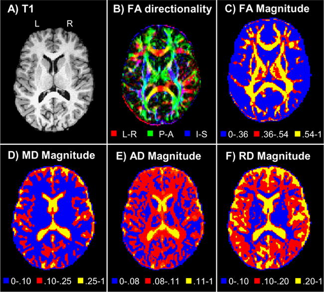
Results obtained from a single subject during the level-one DTI analyses. Panel A shows the anatomical structure (i.e., white matter, gray matter and cerebral spinal fluid boundaries) derived from the T1 map of a selected subject. All data is presented in neurological view as indicated by the left (L) and right (R) hemisphere markings. Panel B shows the principal direction of diffusion, color coded for either the left-right axis (L-R; red), posterior-anterior axis (P-A; green) or inferior-superior axis (I-S; blue). The remaining four panels (C, D, E, and F) respectively correspond to FA, MD, AD and RD magnitude. The color scales were selected to best contrast the anatomical structure for each of the different scalar values.

$$\left[\begin{array}{l}{R}_{int}\hfill \\ G_{int}\hfill \\ B_{int}\hfill \end{array}\right]=255·FA·\mathit{abs}\left(\left[\begin{array}{l}{E}_{L-R}\hfill \\ E_{P-A}\hfill \\ E_{I-S}\hfill \end{array}\right]\right)$$ (10)

were E corresponds to the eigenvector values at each axis L-R (left-right), P-A (posterior-anterior) and I-S (inferior-superior), and R_int, G_int, B_int represent the color map used for display. The remaining panels correspond to the magnitude of FA, MD, AD and RD for the same subject. Each image was scaled to have a maximum value of 255, and color coding scales were selected to best contrast the different anatomical structures where appropriate. All four scalar values were then subjected to separate J-ICA analyses to determine the relationship between the scalars and our measure of gray matter connectivity (DMN).

C. Joint ICA

The final section describes the results from the four separate J-ICA analyses. The first J-ICA used the 24 individual subjects’ back-reconstructed DMN components and their associated FA maps to test our primary hypothesis that functional connectivity in the gray matter during resting state would be dependent on the integrity of connectivity (FA values) between the two hemispheres. The resulting output from this J-ICA was 21 joint FMRI/FA components. An identical spatial correlation algorithm was then applied to the 21 resulting FMRI components to select the component that best matched the spatial topography of the DMN as indicated by our ideal mask. Results indicated that the component which correlated the highest with our ideal mask (r = 0.3761) was more than 3 standard deviations (mean for all components = 0.0303 ± 0.1027) above the spatial correlations for the remaining components (range = −0.1513 to 0.1207). Areas (z = 1.986; volume > 0.440 ml) of the DMN component were similar to those previously identified in the group ICA analysis, with the exception of an additional cluster and relatively larger volumes (more regions) of activation (see Fig. 6). The additional cluster was located in the left middle temporal gyrus (BA 21) and the left superior temporal gyrus (cluster 5). The J-ICA indicated several white matter tracts where the degree of anisotropy (FA values) was associated with shared variance with the DMN. These two fiber tracts included the entirety of the corpus callosum (rostrum, genu, body and splenium) and the cingulate bundles bilaterally.

Fig. 6.

The output of the J-ICA examining shared variance between individual subject’s default mode network (DMN) and FA voxel-wise maps. The spatial activation map corresponds to the component which had the highest correlation with the ideal mask. Regions of the selected DMN component included 1) the anterior cingulate gyrus, 2) the posterior cingulate gyrus, the 3) left and 4) right posterior parietal lobe with associated cortical areas, and the 5) left superior temporal gyrus. The FA component associated with the DMN included activation of the entire corpus callosum and the bilateral cingulate bundles (c). Highlighted regions from the corpus callosum include the (a) rostrum and the (b) splenium. Axial (Z) and sagittal (X) slice locations are presented according to the origin in Talairach space and the two hemispheres are labeled for right (R) and left (L). Only the voxels with the highest z-scores (>5%) in the resulting DMN (warm colorings) and FA (cold colorings) components are displayed. For the DMN component the red coloring corresponds to voxels that had a z value ranging from 1% to 5% (2.0 ≤ z < 3.8), whereas the yellow coloring corresponds to voxels whose z values were greater than 1% (z ≥ 3.8). As for the FA component the dark blue coloring corresponds to voxels that had a z value ranging from 1% to 5% (1.8 ≤ z < 3.0), whereas the cyan coloring corresponds to voxels whose z values were greater than 1% (z ≥ 3.0).

The remaining J-ICA analyses were based on the individual subject’s DMN components and the three remaining scalar maps (MD, AD, and RD) derived from the DTI analyses. For each of these J-ICA analyses, FMRI results indicated a single component that was highly correlated with the ideal mask compared to the remaining components. Specifically, in the MD analyses the selected DMN component had a correlation of r = 0.3656 (mean = 0.0527±0.0943) with the ideal mask, which was more than three standard deviations above the correlations obtained with the remaining components (range = −0.0846 to 0.1633). Similar results were obtained for the DMN component obtained in the AD (r = 0.4006; mean = 0.0394 ± 0.1053; remaining components range = −0.0713 to 0.1635) and RD (r = 0.3423; mean = 0.0642 ± 0.0843; remaining components range = −0.0333 to 0.1645) J-ICAs. These results highlight the reliability of our methodology in selecting a DMN component across all four J-ICAs. As the clusters of the DMN were extremely similar to both the group ICA data and the J-ICA with FA, the individual anatomical locations are not reported to reduce redundancy.

In contrast to the J-ICA of DMN and FA map, the results from the other three J-ICAs of combining the scalar measures were not associated with any significant clusters in the white tracts. Instead, the majority of the activity for the MD and AD components was localized to regions that have high concentrations of CSF such as the ventricles and the longitudinal sinus. This was also true for the J-ICA involving RD, with the exception that a few significant clusters of activity were observed in prefrontal gray matter areas.

D. Supplementary Analyses

Finally, a supplementary analysis was performed to better characterize the direction of effects for the J-ICA involving the DMN and FA maps. Specifically, we correlated the average FA values in the corpus callosum/cingulate bundles with the average z scores from the DMN. For both measures, the masks for the supplementary analyses were constructed by thresholding the individual voxels in the resulting joint components based on the top 5% z-scores of the voxels inside the brain (for voxels meeting this criteria refer to Fig. 6). An outlier analysis identified one subject whose FA scores were more than 3 standard deviations below the mean. This subject’s data was subsequently excluded from the analysis. The resulting correlation indicated that a significant, positive relationship existed between the magnitude of FA values in corpus callosum and cingulate bundles and the magnitude of activity in the DMN network (r = 0.43; p < 0.05).

IV. Discussion

Signal processing techniques play an important role in elucidating the nature of the signals that underlie neuronal functioning and ultimately human behavior. These roles range from the determination of the pulse sequence parameters (e.g., fat suppression pulses) and processing techniques (e.g., Fast Fourier Transforms) used to acquire and reconstruct the raw imaging data through sophisticated techniques to fuse the information obtained across different imaging modalities. Previous work has demonstrated how J-ICA can be used to combine FMRI data with structural data [66], EEG [50] and genetic information [67]. The current application has extended this work by demonstrating the unique information that can be obtained when information from two different signal sources of connectivity are combined. Specifically, we demonstrate how signal processing techniques can be used to combine information about gray (FMRI) and white (DTI) matter connectivity in a purely data-driven fashion. Our results demonstrate that the fusion of information from different imaging modalities and tissue types can be synergistic and critical for understanding how the brain functions as a system.

Current results indicated that there was shared variance between the DMN and the degree of anisotropic diffusion (FA) in the corpus callosum and the cingulate bundle. Specifically, the magnitude of DMN activation was positively correlated with the magnitude of anisotropic diffusion in these two white matter structures. In contrast, there were no significant regions that exhibited a relationship between the DMN and measures of mean diffusivity (MD), more direct markers of axonal diffusivity (AD) and myelin integrity (RD). The corpus callosum is the major white matter fiber bundle linking the two cerebral hemispheres, and is comprised of more than 300 million individual tracts [70]. It is crucial for interhemispheric integration and communication [69]. A wide range of studies have reported positive correlations between measures of callosal thickness and measures of higher cognitive functioning in healthy control subjects [70] and clinical patient cohorts [71;72], supporting the integrative role of the corpus callosum in coordinating cortical activity across hemispheres. The cingulate bundles, located just superior to the corpus callosum, are white matter bundles that run longitudinally within each hemisphere and connect anterior (executive) and posterior (sensory) communication centers of the brain. Collectively, current results indicate that resting measures of gray matter connectivity (DMN) are most dependent on the integrity of white matter connections both within and between the two hemispheres.

Current results also highlight the capabilities of J-ICA in detecting shared variance across disparate signals arising from different tissue sources. To our knowledge, this is a unique extension of J-ICA, given that previous applications [45;50;66] have predominantly focused on signals that arise from the same tissue source (i.e., gray matter), which are more likely to have similar signal properties. Moreover, the current application represents the first J-ICA application that was based on a completely data-driven pipeline and not dependent on human intervention. To date, the most widely used technique for selecting the DMN from the set of randomly ordered ICA components is visual inspection followed by manual selection. However, this processing is time consuming and prone to human error. By spatially correlating the resulting component with an ideal mask, we were able to fully automate our J-ICA pipeline to optimize processing efficiency. Finally, the current application demonstrates the superiority of J-ICA in discovering co-varying signals that would be missed in standard univariate analytic techniques that are employed in a vast majority of imaging studies.

Various signal processing strategies have been widely employed in both FMRI and DTI data analyses. In the current application, the necessary steps to perform a complete data-driven analysis of these two imaging modalities have been described. Although the most current signal processing techniques were used in the study, there is still potential for improvement and optimization. Specifically, FMRI and DTI are both imaging modalities that are characterized by a low signal-to-noise ratio (SNR). Despiking, blurring and data averaging are a few examples of the signal processing techniques that were used to increase the SNR in the current experiment. However, other techniques, such as the filtering of FMRI signals in the temporal domain or wavelet transformations, could have been applied to the data to increase the signal and/or decrease noise. Furthermore, a careful study examining the effects of varying different parameters from each of the signal processing steps (e.g., varying the blurring kernel size, altering the parameters for despiking, changing the cost function in registration algorithms) could also be undertaken to maximize signal strength. Also, the ICA methods employed in this paper assumed that the data was linear, which is likely not entirely true. Non-linear ICA techniques could therefore be developed to perform group and J-ICA, which may ultimately be better matched towards signal properties. Finally, future extensions could include a multi-dimensional J-ICA of different tissue types (gray and white) as well as signal sources (hemodynamic and electrophysiological).

In summary, more advanced signal processing techniques such as ICA have only recently been applied to the analyses of neural connectivity. This technique has already provided important information about various cognitions and disorders [31], and has the additional advantage of not relying on a priori assumptions regarding the expected spatial and temporal pattern of activation. In the current paper we have replicated the finding that ICA can be used to determine indices of functional connectivity during the resting state (DMN) when an a priori model of expected activation does not exist (i.e., a standard GLM analysis). We have extended this work with J-ICA by demonstrating that the magnitude of functional connectivity in the DMN is dependent on the magnitude of anisotropic diffusion in the corpus callosum and cingulate bundles. The simultaneous determination of white and gray matter connectivity may be especially important for clinical populations such as schizophrenia, in which disturbances in functional connectivity are posited to play a major role in observed behavioral and cognitive dysfunction.

Biographies

Alexandre R. Franco received his Electrical Engineer degree with emphasis in telecommunications from Pontifícia Universidade Católica do Rio Grande do Sul, Brazil, in 2003, and master’s degree in Electrical Engineering from the University of New Mexico, Albuquerque, in 2005. He is currently perusing a Ph.D. degree in Electrical Engineering from the University of New Mexico being advised by Dr. Heileman, were he is expected to graduate in 2009.

Alexandre is currently working as a research assistant at the Mind Research Network under the supervision of Dr. Andrew Mayer. He is an author of 6 peer-reviewed journal articles that have been printed or are currently in press. Alexandre recently attended the Summer School: Mathematics in Brain Imaging at the Institute for Pure & Applied Mathematics, in UCLA, where he received a fellowship from the UCLA Center for Computational Biology. His interests include medical imaging, machine learning, statistical analysis, signal processing and game theory.

Mr. Franco is a student member of IEEE, member of Engineering and Medicine, Biology Society and the Computational Intelligence Society.

Josef Ling received a bachelor’s degree in Sociology from the University of Minnesota, Minnesota, in 1991and is currently pursuing a master’s degree in Biomedical Engineering at the University of New Mexico, New Mexico. Mr. Ling worked for a decade as software engineer before joining the Mind Research Network Neuroinformatics team. Mr. Ling is currently a research assistant and software developer for Dr. Mayer at the Mind Research Network.

Arvind Caprihan received B.Tech. in Electrical Engineering from Indian Institute of Technology, Mumbai, India in 1967 and a Ph.D. in Electrical Engineering from Rice University, Houston in 1972. He taught Biomedical Engineering at COPPE, Universidade Federal de Rio de Janeiro, Brazil from 1972 to 1980. He worked as a Scientist at the Lovelace Respiratory Research Institute in Albuquerque from 1982 to 1994 and then at New Mexico Resonance (NMR), Albuquerque from 1994 to 2006. At Lovelace and at NMR he developed methods of flow and diffusion measurement by magnetic resonance imaging (MRI) with applications to flow of granular matter, applied phosphorus spectroscopy to study metabolism, and developed methods of indirectly measuring porosity of ceramics by imaging fluorinated gases in restricted spaces. He joined the Mind Research Network in 2006. Dr. Caprihan’s interests include applications of MRI techniques such as diffusion tensor imaging (DTI) and functional magnetic resonance imaging (fMRI) to study neurodevelopment in children, and their application to characterize biomarkers of schizophrenia, and addiction. He is currently working on machine learning and pattern classification techniques for combining multimodal neuroimaging data.

Vince D. Calhoun received a bachelor’s degree in Electrical Engineering from the University of Kansas, Lawrence, Kansas, in 1991, master’s degrees in Biomedical Engineering and Information Systems from Johns Hopkins University, Baltimore, in 1993 and 1996, respectively, and the Ph.D. degree in electrical engineering from the University of Maryland Baltimore County, Baltimore, in 2002. He worked as a Senior Research Engineer at the Psychiatric Neuro-Imaging Laboratory at Johns Hopkins from 1993 until 2002. Then he took a position as the director of medical image analysis at the Olin Neuropsychiatry Research Center and an associate professor at Yale University.

Dr. Calhoun is currently Director of Image Analysis and MR Research at the Mind Research Network and is an associate professor in the Dept of ECE, neurosciences, and computer science at the University of New Mexico. He is the author of more than 80 full journal articles, over 200 technical reports, abstracts and conference proceedings. Much of his career has been spent on the development of data driven approaches for the analysis of functional magnetic resonance imaging (fMRI) data. He has multiple NSF and NIH grants on the incorporation of prior information into independent component analysis (ICA) for fMRI, data fusion of multimodal imaging and genetics data, and the identification of biomarkers for disease.

Dr. Calhoun is a senior member of the IEEE, the Organization for Human Brain Mapping, and the International Society for Magnetic Resonance in Medicine. He has participated in multiple NIH study sections. He has worked in the organization of workshops at conferences including the society of biological psychiatry (SOBP) and the international conference of independent component analysis and blind source separation (ICA). He is currently serving on the IEEE Machine Learning for Signal Processing (MLSP) Technical Committee and has previous served as the general chair of the 2005 meeting. He is a reviewer for a number of international journals and is on the editorial board of the Human Brain Mapping journal and an associate editor for the IEEE Signal Processing Letters and the International Journal of Computational Intelligence and Neuroscience.

Rex Jung is an Assistant Professor of Neurology, Psychology, and Neurosurgery at the University of New Mexico, a Research Scientist at the Mind Research Network, and a Neuroscience Consultant at Sandia National Laboratories in Albuquerque, New Mexico. He received his Ph.D. in Psychology from the University of New Mexico in 2001. His research is designed to relate behavioral measures including intelligence, personality, and creativity, to brain function and structure in healthy, neurological, and psychiatric subjects. He is a clinical neuropsychologist, with specialty practice serving neurosurgery patients.

Gregory L. Heileman received the BA degree from Wake Forest University in 1982, the MS degree in Biomedical Engineering and Mathematics from the University of North Carolina-Chapel Hill in 1986, and the PhD degree in Computer Engineering from the University of Central Florida in 1989. In 1990 he joined the Department of Electrical and Computer Engineering at the University of New Mexico, Albuquerque, NM, where he is currently Professor and Associate Chair. During 1998 he held a research fellowship at the Universidad Carlos III de Madrid, and in 2005 he held a similar position at the Universidad Politénica de Madrid.

Andrew R. Mayer received a BA degree from the State University of New York at Buffalo in 1994, a MS degree in Clinical Neuropsychology from the Chicago Medical School in 1998, and his PhD in the same field in 2001. He completed his post-doctoral fellowship in the Department of Neurology at the University of New Mexico School of Medicine. He is currently a Research Scientist at the Mind Research Network in Albuquerque, NM and an adjunct Assistant Professor in the Department of Neurology. His current research interests focus on using functional imaging to study attentional functioning in clinical and healthy populations.

References

- 1.Ramnani N, Behrens TE, Penny W, Matthews PM. New approaches for exploring anatomical and functional connectivity in the human brain. Biol Psychiatry. 2004 Nov;56(9):613–619. doi: 10.1016/j.biopsych.2004.02.004. [DOI] [PubMed] [Google Scholar]
- 2.Roth G, Dicke U. Evolution of the brain and intelligence. Trends Cogn Sci. 2005 May;9(5):250–257. doi: 10.1016/j.tics.2005.03.005. [DOI] [PubMed] [Google Scholar]
- 3.Schmithorst VJ, Wilke M, Dardzinski BJ, Holland SK. Cognitive functions correlate with white matter architecture in a normal pediatric population: a diffusion tensor MRI study. Hum Brain Mapp. 2005 Oct;26(2):139–147. doi: 10.1002/hbm.20149. [DOI] [PMC free article] [PubMed] [Google Scholar]
- 4.Lindenberger U, Mayr U, Kliegl R. Speed and intelligence in old age. Psychol Aging. 1993 June;8(2):207–220. doi: 10.1037//0882-7974.8.2.207. [DOI] [PubMed] [Google Scholar]
- 5.Le Bihan D. Looking into the functional architecture of the brain with diffusion MRI. Nat Rev Neurosci. 2003 June;4(6):469–480. doi: 10.1038/nrn1119. [DOI] [PubMed] [Google Scholar]
- 6.Sen PN, Basser PJ. A model for diffusion in white matter in the brain. Biophys J. 2005 Nov;89(5):2927–2938. doi: 10.1529/biophysj.105.063016. [DOI] [PMC free article] [PubMed] [Google Scholar]
- 7.Beaulieu C. The basis of anisotropic water diffusion in the nervous system - a technical review. NMR Biomed. 2002 Nov;15(7–8):435–455. doi: 10.1002/nbm.782. [DOI] [PubMed] [Google Scholar]
- 8.Basser PJ. New histological and physiological stains derived from diffusion-tensor MR images. Ann N Y Acad Sci. 1997 May;820:123–138. doi: 10.1111/j.1749-6632.1997.tb46192.x. [DOI] [PubMed] [Google Scholar]
- 9.Westin CF, Maier SE, Mamata H, Nabavi A, Jolesz FA, Kikinis R. Processing and visualization for diffusion tensor MRI. Med Image Anal. 2002 June;6(2):93–108. doi: 10.1016/s1361-8415(02)00053-1. [DOI] [PubMed] [Google Scholar]
- 10.Stejskal EO, Tanner JE. Spin diffusion measurements: spin echoes in the presence of a time-dependent field gradient. J Chem Phys. 1965 Jan;42:288–292. [Google Scholar]
- 11.Song SK, Sun SW, Ju WK, Lin SJ, Cross AH, Neufeld AH. Diffusion tensor imaging detects and differentiates axon and myelin degeneration in mouse optic nerve after retinal ischemia. Neuroimage. 2003 Nov;20(3):1714–1722. doi: 10.1016/j.neuroimage.2003.07.005. [DOI] [PubMed] [Google Scholar]
- 12.Bandettini PA, Wong EC, Hinks RS, Tikofsky RS, Hyde JS. Time course EPI of human brain function during task activation. Magn Reson Med. 1992 June;25(2):390–397. doi: 10.1002/mrm.1910250220. [DOI] [PubMed] [Google Scholar]
- 13.Ogawa S, Lee TM, Kay AR, Tank DW. Brain magnetic resonance imaging with contrast dependent on blood oxygenation. Proc Natl Acad Sci U S A. 1990 Dec;87(24):9868–9872. doi: 10.1073/pnas.87.24.9868. [DOI] [PMC free article] [PubMed] [Google Scholar]
- 14.Bandettini P. Functional MRI today. Int J Psychophysiol. 2007 Feb;63(2):138–145. doi: 10.1016/j.ijpsycho.2006.03.016. [DOI] [PubMed] [Google Scholar]
- 15.Friston KJ, Holmes AP, Poline JB, Grasby PJ, Williams SC, Frackowiak RS, Turner R. Analysis of fMRI time-series revisited. Neuroimage. 1995 Mar;2(1):45–53. doi: 10.1006/nimg.1995.1007. [DOI] [PubMed] [Google Scholar]
- 16.Glover GH. Deconvolution of impulse response in event-related BOLD fMRI. Neuroimage. 1999 Apr;9(4):416–429. doi: 10.1006/nimg.1998.0419. [DOI] [PubMed] [Google Scholar]
- 17.Leibovici D, Beckmann C. An Introduction to Multiway Methods for Multi-Subject FMRI. FMRIB Technical Report. 2001 [Google Scholar]
- 18.Beckmann CF, Smith SM. Probabilistic independent component analysis for functional magnetic resonance imaging. IEEE Trans Med Imaging. 2004 Feb;23(2):137–152. doi: 10.1109/TMI.2003.822821. [DOI] [PubMed] [Google Scholar]
- 19.Calhoun VD, Adali T. Unmixing fMRI with independent component analysis. IEEE Eng Med Biol Mag. 2006 Mar;25(2):79–90. doi: 10.1109/memb.2006.1607672. [DOI] [PubMed] [Google Scholar]
- 20.Cardoso JF, Souloumiac A. Blind Beamforming for non Gaussian Signals. IEE- Proc -F. 1993 Dec;140(6):362–370. [Google Scholar]
- 21.Lee TW, Girolami M, Sejnowski TJ. Independent component analysis using an extended infomax algorithm for mixed subgaussian and supergaussian sources. Neural Comput. 1999 Feb;11(2):417–441. doi: 10.1162/089976699300016719. [DOI] [PubMed] [Google Scholar]
- 22.Hyvarinen A, Oja E. Simple neuron models for independent component analysis. Int J Neural Syst. 1996 Dec;7(6):671–687. doi: 10.1142/s0129065796000646. [DOI] [PubMed] [Google Scholar]
- 23.Cruces S, Cichocki A, Amari S. Criteria for the simultaneous blind extraction of arbitrary groups of sources. Proc. Int. Conf. on ICA and BSS; San Diego. 2001. pp. 740–745. [Google Scholar]
- 24.Tong L, Soon VC, Huang YF, Liu R. Indeterminacy and identifiability of blind identification. IEEE Trans Circuits Syst. 1991;38(5):499–509. [Google Scholar]
- 25.Correa N, Adali T, Calhoun VD. Performance of blind source separation algorithms for fMRI analysis using a group ICA method. Magn Reson Imaging. 2007 June;25(5):684–694. doi: 10.1016/j.mri.2006.10.017. [DOI] [PMC free article] [PubMed] [Google Scholar]
- 26.Bell AJ, Sejnowski TJ. An information-maximization approach to blind separation and blind deconvolution. Neural Comput. 1995 Nov;7(6):1129–1159. doi: 10.1162/neco.1995.7.6.1129. [DOI] [PubMed] [Google Scholar]
- 27.Calhoun VD, Adali T, Pearlson GD, Pekar JJ. A method for making group inferences from functional MRI data using independent component analysis. Hum Brain Mapp. 2001 Nov;14(3):140–151. doi: 10.1002/hbm.1048. [DOI] [PMC free article] [PubMed] [Google Scholar]
- 28.Wax M, Kailath T. Detection of signals by information theoretic criteria. IEEE Trans Acoust Speech, Sig Proc. 1985;33:387–392. [Google Scholar]
- 29.Stevens MC, Kiehl KA, Pearlson G, Calhoun VD. Functional neural circuits for mental timekeeping. Hum Brain Mapp. 2007 May;28(5):394–408. doi: 10.1002/hbm.20285. [DOI] [PMC free article] [PubMed] [Google Scholar]
- 30.Buckner RL, Andrews-Hanna JR, Schacter DL. The brain’s default network: anatomy, function, and relevance to disease. Ann N Y Acad Sci. 2008 Mar;1124:1–38. doi: 10.1196/annals.1440.011. [DOI] [PubMed] [Google Scholar]
- 31.Damoiseaux JS, Rombouts SA, Barkhof F, Scheltens P, Stam CJ, Smith SM, Beckmann CF. Consistent resting-state networks across healthy subjects. Proc Natl Acad Sci U S A. 2006 Sept;103(37):13848–13853. doi: 10.1073/pnas.0601417103. [DOI] [PMC free article] [PubMed] [Google Scholar]
- 32.Gusnard DA, Raichle ME. Searching for a baseline: functional imaging and the resting human brain. Nat Rev Neurosci. 2001 Oct;2(10):685–694. doi: 10.1038/35094500. [DOI] [PubMed] [Google Scholar]
- 33.Raichle ME, MacLeod AM, Snyder AZ, Powers WJ, Gusnard DA, Shulman GL. A default mode of brain function. Proc Natl Acad Sci U S A. 2001 Jan;98(2):676–682. doi: 10.1073/pnas.98.2.676. [DOI] [PMC free article] [PubMed] [Google Scholar]
- 34.Shulman GL, Fiez JA, Corbetta M, Buckner RL, Miezin FM, Raichle ME, Petersen SE. Common blood flow changes across visual tasks. 2. Decreases in cerebral cortex. J Cogn Neurosci. 1997 Sept;9(5):648–663. doi: 10.1162/jocn.1997.9.5.648. [DOI] [PubMed] [Google Scholar]
- 35.Binder JR, Frost JA, Hammeke TA, Bellgowan PS, Rao SM, Cox RW. Conceptual processing during the conscious resting state. A functional MRI study. J Cogn Neurosci. 1999 Jan;11(1):80–95. doi: 10.1162/089892999563265. [DOI] [PubMed] [Google Scholar]
- 36.Laufs H, Holt JL, Elfont R, Krams M, Paul JS, Krakow K, Kleinschmidt A. Where the BOLD signal goes when alpha EEG leaves. Neuroimage. 2006 July;31(4):1408–1418. doi: 10.1016/j.neuroimage.2006.02.002. [DOI] [PubMed] [Google Scholar]
- 37.Fox MD, Snyder AZ, Vincent JL, Corbetta M, Van E, Raichle ME. The human brain is intrinsically organized into dynamic, anticorrelated functional networks. Proc Natl Acad Sci U S A. 2005 July;102(27):9673–9678. doi: 10.1073/pnas.0504136102. [DOI] [PMC free article] [PubMed] [Google Scholar]
- 38.Fransson P. Spontaneous low-frequency BOLD signal fluctuations: an fMRI investigation of the resting-state default mode of brain function hypothesis. Hum Brain Mapp. 2005 Sept;26(1):15–29. doi: 10.1002/hbm.20113. [DOI] [PMC free article] [PubMed] [Google Scholar]
- 39.Greicius MD, Krasnow B, Reiss AL, Menon V. Functional connectivity in the resting brain: a network analysis of the default mode hypothesis. Proc Natl Acad Sci U S A. 2003 Jan;100(1):253–258. doi: 10.1073/pnas.0135058100. [DOI] [PMC free article] [PubMed] [Google Scholar]
- 40.Franco AR, Pritchard A, Calhoun VC, Mayer AR. Inter-rater and Inter-method Reliability of Default Mode Network Selection. Human Brain Mapping. doi: 10.1002/hbm.20668. to be published. [DOI] [PMC free article] [PubMed] [Google Scholar]
- 41.Raichle ME, Snyder AZ. A default mode of brain function: a brief history of an evolving idea. Neuroimage. 2007 Oct;37(4):1083–1090. doi: 10.1016/j.neuroimage.2007.02.041. [DOI] [PubMed] [Google Scholar]
- 42.Gilbert SJ, Dumontheil I, Simons JS, Frith CD, Burgess PW. Comment on “Wandering minds: the default network and stimulus-independent thought”. Science. 2007 July ;317(5834):43. doi: 10.1126/science.317.5834.43. [DOI] [PubMed] [Google Scholar]
- 43.Mason MF, Norton MI, Van Horn JD, Wegner DM, Grafton ST, Macrae CN. Wandering minds: the default network and stimulus-independent thought. Science. 2007 Jan;315(5810):393–395. doi: 10.1126/science.1131295. [DOI] [PMC free article] [PubMed] [Google Scholar]
- 44.Calhoun VD, Adali T, Giuliani NR, Pekar JJ, Kiehl KA, Pearlson GD. Method for multimodal analysis of independent source differences in schizophrenia: combining gray matter structural and auditory oddball functional data. Hum Brain Mapp. 2006 Jan;27(1):47–62. doi: 10.1002/hbm.20166. [DOI] [PMC free article] [PubMed] [Google Scholar]
- 45.Choi K, Craddock RC, Holtzheimer PE, Yang Z, Hu XP, Mayberg HS. Proc Intl Soc Mag Reson Med. Vol. 16. Toronto CA: 2008. A Combined Functional-Structural Connectivity Analysis of Major Depression Using Joint-ICA; p. #3555. [Google Scholar]
- 46.Friston K. Learning and inference in the brain. Neural Netw. 2003 Nov;16(9):1325–1352. doi: 10.1016/j.neunet.2003.06.005. [DOI] [PubMed] [Google Scholar]
- 47.Friston K, Poline JP, Strother S, Holmes A, Frith CD, Frackowiak RS. A Multivariate analysis of PET activation studies. Hum Brain Map. 1996;4:140–151. doi: 10.1002/(SICI)1097-0193(1996)4:2<140::AID-HBM5>3.0.CO;2-3. [DOI] [PubMed] [Google Scholar]
- 48.McIntosh AR, Bookstein FL, Haxby JV, Grady CL. Spatial pattern analysis of functional brain images using partial least squares. Neuroimage. 1996 June;3(3 Pt 1):143–157. doi: 10.1006/nimg.1996.0016. [DOI] [PubMed] [Google Scholar]
- 49.Dale AM, Halgren E. Spatiotemporal mapping of brain activity by integration of multiple imaging modalities. Curr Opin Neurobiol. 2001 Apr;11(2):202–208. doi: 10.1016/s0959-4388(00)00197-5. [DOI] [PubMed] [Google Scholar]
- 50.Calhoun VD, Adali T, Pearlson GD, Kiehl KA. Neuronal chronometry of target detection: fusion of hemodynamic and event-related potential data. Neuroimage. 2006 Apr;30(2):544–553. doi: 10.1016/j.neuroimage.2005.08.060. [DOI] [PubMed] [Google Scholar]
- 51.Reese TG, Heid O, Weisskoff RM, Wedeen VJ. Reduction of eddy-current-induced distortion in diffusion MRI using a twice-refocused spin echo. Magn Reson Med. 2003 Jan;49(1):177–182. doi: 10.1002/mrm.10308. [DOI] [PubMed] [Google Scholar]
- 52.Ardekani, Sinha U. Quantitative assessment of parallel acquisition techniques in diffusion tensor imaging at 3.0 Tesla. Conf Proc IEEE Eng Med Biol Soc. 2004;2:1072–1075. doi: 10.1109/IEMBS.2004.1403349. [DOI] [PubMed] [Google Scholar]
- 53.Cox RW. AFNI: software for analysis and visualization of functional magnetic resonance neuroimages. Comput Biomed Res. 1996 June;29(3):162–173. doi: 10.1006/cbmr.1996.0014. [DOI] [PubMed] [Google Scholar]
- 54.Calhoun VD. Group ICA of fMRI Toolbox (GIFT) 2004 [Google Scholar]
- 55.Jenkinson M, Bannister P, Brady M, Smith S. Improved optimization for the robust and accurate linear registration and motion correction of brain images. Neuroimage. 2002 Oct;17(2):825–841. doi: 10.1016/s1053-8119(02)91132-8. [DOI] [PubMed] [Google Scholar]
- 56.Ardekani BA, Bachman AH, Helpern JA. A quantitative comparison of motion detection algorithms in fMRI. Magn Reson Imaging. 2001 Sept;19(7):959–963. doi: 10.1016/s0730-725x(01)00418-0. [DOI] [PubMed] [Google Scholar]
- 57.Cox RW, Jesmanowicz A. Real-time 3D image registration for functional MRI. Magn Reson Med. 1999 Dec;42(6):1014–1018. doi: 10.1002/(sici)1522-2594(199912)42:6<1014::aid-mrm4>3.0.co;2-f. [DOI] [PubMed] [Google Scholar]
- 58.Parrish T. Functional MR imaging. Magn Reson Imaging Clin N Am. 1999 Nov;7(4):765–82. vi. [PubMed] [Google Scholar]
- 59.Talairach J, Tournoux P. Co-planar stereotaxic atlas of the human brain. New York: Thieme; 1988. [Google Scholar]
- 60.Li YO, Adali T, Calhoun VD. Estimating the number of independent components for functional magnetic resonance imaging data. Hum Brain Mapp. 2007 Nov;28(11):1251–1266. doi: 10.1002/hbm.20359. [DOI] [PMC free article] [PubMed] [Google Scholar]
- 61.McKeown MJ, Makeig S, Brown GG, Jung TP, Kindermann SS, Bell AJ, Sejnowski TJ. Analysis of fMRI data by blind separation into independent spatial components. Hum Brain Mapp. 1998;6(3):160–188. doi: 10.1002/(SICI)1097-0193(1998)6:3<160::AID-HBM5>3.0.CO;2-1. [DOI] [PMC free article] [PubMed] [Google Scholar]
- 62.Foreman SD, Cohen JD, Fitzgerald M, Eddy WF, Mintun MA, Noll DC. Improved assessment of significant activation in functional magnetic resonance imaging (fMRI): Use ofImproved assessment of significant a cluster-size threshold. Magn Reson Med. 1995;33:636–647. doi: 10.1002/mrm.1910330508. [DOI] [PubMed] [Google Scholar]
- 63.Koay CG, Carew JD, Alexander AL, Basser PJ, Meyerand ME. Investigation of anomalous estimates of tensor-derived quantities in diffusion tensor imaging. Magn Reson Med. 2006 Apr;55(4):930–936. doi: 10.1002/mrm.20832. [DOI] [PubMed] [Google Scholar]
- 64.Jones DK, Symms MR, Cercignani M, Howard RJ. The effect of filter size on VBM analyses of DT-MRI data. Neuroimage. 2005 June;26(2):546–554. doi: 10.1016/j.neuroimage.2005.02.013. [DOI] [PubMed] [Google Scholar]
- 65.Cordes D, Haughton VM, Arfanakis K, Carew JD, Turski PA, Moritz CH, Quigley MA, Meyerand ME. Frequencies contributing to functional connectivity in the cerebral cortex in “resting-state” data. AJNR Am J Neuroradiol. 2001 Aug;22(7):1326–1333. [PMC free article] [PubMed] [Google Scholar]
- 66.Calhoun V, Adali T, Liu J. A feature-based approach to combine functional MRI, structural MRI and EEG brain imaging data. Conf Proc IEEE Eng Med Biol Soc. 2006;1:3672–3675. doi: 10.1109/IEMBS.2006.259810. [DOI] [PubMed] [Google Scholar]
- 67.Liu J, Pearlson G, Windemuth A, Ruano G, Perrone-Bizzozero NI, Calhoun V. Combining fMRI and SNP data to investigate connections between brain function and genetics using parallel ICA. Hum Brain Mapp. 2007 Dec; doi: 10.1002/hbm.20508. [DOI] [PMC free article] [PubMed] [Google Scholar]
- 68.Hofer S, Frahm J. Topography of the human corpus callosum revisited--comprehensive fiber tractography using diffusion tensor magnetic resonance imaging. Neuroimage. 2006 Sept;32(3):989–994. doi: 10.1016/j.neuroimage.2006.05.044. [DOI] [PubMed] [Google Scholar]
- 69.Schlaug G, Jancke L, Huang Y, Staiger JF, Steinmetz H. Increased corpus callosum size in musicians. Neuropsychologia. 1995 Aug;33(8):1047–1055. doi: 10.1016/0028-3932(95)00045-5. [DOI] [PubMed] [Google Scholar]
- 70.Hulshoff Pol HE, Schnack HG, Mandl RC, Brans RG, van Haren NE, Baare WF, van Oel CJ, Collins DL, Evans AC, Kahn RS. Gray and white matter density changes in monozygotic and same-sex dizygotic twins discordant for schizophrenia using voxel-based morphometry. Neuroimage. 2006 June;31(2):482–488. doi: 10.1016/j.neuroimage.2005.12.056. [DOI] [PubMed] [Google Scholar]
- 71.Atkinson DS, Jr, bou-Khalil B, Charles PD, Welch L. Midsagittal corpus callosum area, intelligence, and language dominance in epilepsy. J Neuroimaging. 1996 Oct;6(4):235–239. doi: 10.1111/jon199664235. [DOI] [PubMed] [Google Scholar]
- 72.Strauss E, Wada J, Hunter M. Callosal morphology and performance on intelligence tests. J Clin Exp Neuropsychol. 1994 Feb;16(1):79–83. doi: 10.1080/01688639408402618. [DOI] [PubMed] [Google Scholar]