A multivariate likelihood SIRAS function for phasing and model refinement

The application of a multivariate likelihood function to a single isomorphous replacement with anomalous scattering experiment improves phasing and automated model building with iterative refinement in the test cases shown.

Abstract

A likelihood function based on the multivariate probability distribution of all observed structure-factor amplitudes from a single isomorphous replacement with anomalous scattering experiment has been derived and implemented for use in substructure refinement and phasing as well as macromolecular model refinement. Efficient calculation of a multidimensional integration required for function evaluation has been achieved by approximations based on the function’s properties. The use of the function in both phasing and protein model building with iterative refinement was essential for successful automated model building in the test cases presented.

1. Introduction

Despite the dramatic increase in the number of macromolecular structures in the Protein Data Bank (PDB; Berman et al., 2000 ▶) phased by molecular replacement, about 20% of recently determined crystal structures have still been solved by experimental phasing methods (Long et al., 2008 ▶) phased by molecular replacement. Experimental phase information can also serve as an additional source of information in model building and refinement, especially at lower resolutions when the observation-to-parameter ratio is very low (DeLaBarre & Brunger, 2006 ▶). Recent developments in heavy-atom soaking (Boggon & Shapiro, 2000 ▶; Wernimont et al., 2000 ▶; Dauter et al., 2000 ▶, 2001 ▶; Szczepanowski et al., 2005 ▶; Beck et al., 2008 ▶) have increased the success rate and extended the application of both single-wavelength anomalous diffraction (SAD) and single isomorphous replacement with anomalous scattering (SIRAS). These techniques are often applied to large molecular complexes or flexible molecules, which typically provide fragile crystals and weak diffraction data with a small signal-to-noise ratio. Improved statistical techniques that exploit all information simultaneously are needed to optimally extract information from such data. Furthermore, the enhanced exploitation of SIRAS data from a native and a soaked crystal may lead to solutions which elude SAD data collected from a soaked crystal alone.

The SIRAS experiment involves data collected from a native crystal and Friedel mates from a derivative crystal containing a ‘heavy atom’ [for a review of SIRAS and experimental phasing, see Taylor (2003 ▶) and references therein],

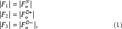with the corresponding model structure factors

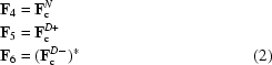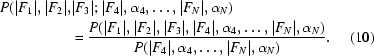
[for simplicity, both the D (derivative) superscript and the complex-conjugate sign will be omitted]. Currently, the best approach for SIRAS substructure phasing and refinement neglects the correlation between the isomorphic and anomalous sources of information. Indeed, the (univariate) likelihood-based SIRAS function used in SHARP (de La Fortelle & Bricogne, 1997 ▶) and BP3 (Pannu et al., 2003 ▶) assumes the independence of a Gaussian term involving anomalous differences (North, 1965 ▶; Matthews, 1966 ▶) and a Rice function modelling the isomorphic data for acentric reflections,

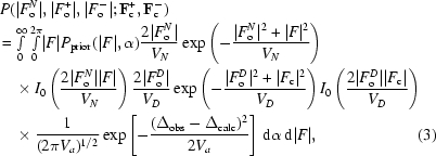where the ‘true’ native amplitude |F| and phase α are integrated out, P _prior describes the prior knowledge about F (if any), F _o ^D is the average of |F _o ⁺|, |F _o ⁻| and |F _c| is the average of |F _c ⁺|, |F _c ⁻|, the calculated structure factors determined from the ‘true’ native structure factor and the calculated heavy-atom structure factors. Δ_obs is the Bijvoet difference of the observed Friedel pairs |F _o ⁺| and |F _o ⁻|, V _N, V _D and V _a are variances and Δ_calc = |F _c ⁺| − |F _c ⁻| is the calculated Bijvoet difference.

Previously, we have shown that substructure phasing and refinement using a multivariate likelihood function that directly considers the correlation between Friedel pairs in a SAD experiment provides better results than the same Gaussian-based term using anomalous differences (Pannu & Read, 2004 ▶; Ness et al., 2004 ▶). Thus, a multivariate function which directly accounts for all correlations between structure factors in a SIRAS experiment should allow the extraction of more information from low signal-to-noise data.

Currently, a function that simultaneously and directly exploits native and derivative data from a SIRAS experiment has not been implemented in macromolecular refinement. The best available approach for considering phase information from a SIRAS experiment in model refinement is with the ‘MLHL’ target function, a univariate likelihood function which incorporates experimental phase information via Hendrickson–Lattman coefficients (Pannu et al., 1998 ▶). How­ever, this indirect use of experimental phases suffers from shortcomings such as the assumption of independence of experimental phase information from the model, an inability for simultaneous refinement of (a perhaps updated) sub­structure and protein models and a dependency on the accuracy and reliability of the phasing program used to generate the Hendrickson–Lattman coefficients (Skubák et al., 2004 ▶). A multivariate single anomalous diffraction (SAD) function has been shown to overcome these shortcomings and to extend the resolution and phase-quality limits needed for successful automated model building with iterative refinement against the SAD data set (Skubák et al., 2005 ▶). In this paper, a multivariate likelihood function for macromolecular refinement against SIRAS experimental data is presented.

2. Method

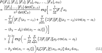
The probability distribution of three structure-factor amplitudes for a reflection [as specified by (1)] given N − 3 model structure factors is derived in Appendix A . In our current implementation, three models specified by (2) are used, leading to the following probability distribution:

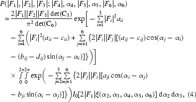where

C₆ is the covariance matrix of the complex Gaussian distribution P(F ₁, …, F ₆), with the real and imaginary components of its inverse denoted as a_jk and b_jk, respectively. Similarly, C₃ is the covariance matrix of the Gaussian distribution P(F ₄, F ₅, F ₆), with the real and imaginary components of its inverse denoted as c_ij and d_ij, respectively.

We define the SIRAS function as the sum over all reflections of the minus logarithm of the derived probability distribution (4). Evaluation of the function requires a three-dimensional integration over the unknown observed phases, one of which is solved analytically (Appendix A ). Since we were not able to find a usable analytical solution to the remaining two integrals, a two-dimensional numerical integration was used for evaluation of the remaining two integrals. However, a SIRAS function employing an integral evaluated by the Gaussian method, as a two-dimensional extension from an accurate implementation of the one-dimensional SAD numerical integration, required up to 1000 × 1000 nodes to achieve an acceptable precision and stable refinement. Clearly, more advanced approximations were needed to speed up the SIRAS function evaluation and to achieve a speed comparable with the currently used functions. The solution adopted is based on analysis of the specific properties of the integral.

In Appendix C , we show that the three-dimensional SIRAS integral I(α₁, α₂, α₃) (before analytical integration) is dependent on nine real-valued parameters (denoted as ennead ): six w parameters (analogous to vector amplitudes) and three ϕ parameters (analogous to vector angles). If the values of the w parameters are small, the surface of the function I(α₁, α₂, α₃) (for a given ) is flat and a small number of sampling points over the whole integration range is sufficient for reasonable precision of the numerical integration of I. However, higher values of the w parameters generally give rise to a sharp and high peak and very dense integration sampling would be required to sample over the whole integration area. Therefore, the position of the peak of the integrand in three-dimensional space (α₁, α₂, α₃) is important for numerical integration of I.

The statement in Appendix D provides a partial localization of the position of the maximum of I: the maximum is close to a certain plane for the majority of reflections in a typical SIRAS experiment. The statement defines the plane and provides the maximal distance of the maximum from the plane. This information can be used to limit the large number of sampling points needed for the numerical integration for large w parameters. A transformation of the coordinate system α₁, α₂, α₃ can be performed such that one of the new coordinate axes is perpendicular to the plane. Sampling of this variable over a short range covering the peak within the maximal distance given by the statement then provides an efficient method for the numerical integration. The transformation and the com­plete algorithm for the SIRAS function evaluation are specified in Appendix E.

The SIRAS function was implemented according to this algorithm in the refinement program REFMAC5 (Murshudov et al., 1997 ▶). Validation of the implementation of the function evaluation in terms of precision and actual number of nodes used has been performed on several SIRAS data sets, showing that a relative precision of the order of 10⁻⁵ is achieved by the use of an average of 100–150 Gaussian integration nodes per reflection.

The SIRAS function has been implemented in REFMAC5 (v.5.6) for substructure refinement and phasing and also for protein refinement with the direct use of SIRAS phase information. The performance of the ‘multivariate’ phasing function has been compared with the currently used univariate function as implemented in the program BP3 (v.1.01), denoted below by ‘univariate’. The function for protein model refinement has been compared against the ‘Rice’ likelihood function lacking prior phase information (Bricogne & Irwin, 1996 ▶; Murshudov et al., 1997 ▶; Pannu & Read, 1996 ▶) denoted below as Rice, and the likelihood function encoding prior phase information with Hendrickson–Lattman coefficients, denoted below as MLHL, both implemented in REFMAC5 (v.5.6) in the context of automated model building with iterative refinement by ARP/wARP (v.7.0; Perrakis et al., 1999 ▶).

For the three SIRAS test cases described below, the CRANK suite (v.1.2.1; Ness et al., 2004 ▶) from CCP4 (v.6.10; Collaborative Computational Project, Number 4, 1994 ▶) was used for automatic structure solution starting with the SIRAS data and the protein sequence. CRANK uses the programs SHELXD (Sheldrick, 2008 ▶) or CRUNCH2 (de Graaff et al., 2001 ▶) for substructure detection, SHELXE (Sheldrick, 2008 ▶) for hand determination, BP3 or REFMAC5 for substructure refinement and phasing, SOLOMON (Abrahams & Leslie, 1996 ▶) for density modification and ARP/wARP for automated model building with iterative refinement by REFMAC5. EMMA from the CCTBX toolbox (Grosse-Kunstleve et al., 2002 ▶) was used to transform all substructure sites to the same origin as the final published model. This simplified the calculation of map correlations with the final map in SFTOOLS (Bart Hazes, unpublished work). Unless otherwise stated, the default CRANK parameters were used in all runs.

The Hendrickson–Lattman coefficients required for the MLHL function were derived using the phasing program in a given pipeline (either BP3 or REFMAC5). MLHL with Hendrickson–Lattman coefficients from the density-modification programs SOLOMON and DM (Cowtan, 1999 ▶) was also tested, but produced poorer results. When the SIRAS function was used for protein refinement, the refined sub­structures from BP3 or REFMAC5 were input into ARP/wARP. For all likelihood functions and test cases, 200 cycles (four times the default) of automated model building with iterative structure refinement were performed to allow con­vergence of the model-building process. The native data were used for model building and refinement in all the test cases (except for the SIRAS function, which used all observations). The resulting models were compared with the final refined structure by a compare-protein script (S. Ness & P. Skubak, unpublished work) from the CRANK suite, which provides the number of ‘correctly built’ residues. A residue is regarded as correctly built if its C^α atom lies within 1 Å of a C^α position from the final model (Badger, 2003 ▶).

All the data sets used for the tests described below were acquired from the PDB. Since the PDB stores reflection data in mmCIF format, conversion to MTZ format was required. The conversion was performed in several steps: firstly, the downloaded mmCIF file was manually analyzed to separate, by hand, the multiple data sets (native, derivative plus and derivative minus) into multiple mmCIF files. The separated mmCIF files were converted using either the CIF2MTZ utility from the CCP4 suite or SF-CONVERT (http://sw-tools.pdb.org/apps/SF-CONVERT) depending on how the anomalous data were represented in the mmCIF file. Finally, the separated MTZ data sets were merged into a single MTZ file using SFTOOLS from CCP4.

3. Results

3.1. DNA-packaging protein Gp17

The initial phases for bacteriophage T4 gp17 ATPase domain mutant complexed with ATP (PDB code 2o0h; Sun et al., 2007 ▶) were determined from a native data set and a selenomethionine derivative containing eight Se atoms collected at the selenium absorption edge. Although the theoretical value of the anomalous scattering coefficient f′′ for an Se atom at its peak is close to 4, a value of 12 was used for the structure determination by the authors (Sun, personal communication). Because of this large discrepancy, we investigated the effects of f′′ on the phasing by running a series of phasing jobs starting from the same substructure and varying f′′ for both functions. As Table 1 ▶ documents, the multivariate function provides almost equally good results in the whole f′′ range from 3 to 16, while the univariate-function results deteriorate with an f′′ lower than 6. Since the value of 12 suggested by the original authors provided close to optimal results for both functions, it was used in all the pipelines (Tables 2 ▶ and 3 ▶).

Table 1. The effect of the f′′ used for phasing on the resulting map correlation after phasing for the 2o0h data set.

	f′′
Map correlation	3	4	6	8	10	12	14	16
Univariate	0.333	0.355	0.379	0.392	0.396	0.397	0.395	0.385
Multivariate	0.405	0.412	0.414	0.413	0.409	0.412	0.414	0.413

Table 2. The map correlations after phasing and density modification (DM).

	2o0h		2b78		2b79
Map correlation after	Phasing	DM	Phasing	DM	Phasing	DM
Univariate	0.397	0.366	0.368	0.488	0.457	0.718
Multivariate	0.412	0.429	0.374	0.535	0.486	0.739

Table 3. The number of residues built using various target functions in phasing and model building.

		Correctly built residues
Phasing function	Refinement function	2o0h	2b78	2b79
Univariate	Rice	24	51	139
Univariate	MLHL	34	96	197
Univariate	Multivariate SIRAS	53	345	235
Multivariate	Rice	68	106	190
Multivariate	MLHL	128	341	201
Multivariate	Multivariate SIRAS	310	353	238

The structure contains a single monomer with 357 residues in the asymmetric unit, a majority of which were correctly built by CRANK using the multivariate SIRAS function for both phasing and protein refinement. Only small fragments of the structure were built using any other combination of the functions for phasing and protein refinement (Table 3 ▶). Fig. 1 ▶ demonstrates the differences in the performance of different refinement target functions in a refinement-only pass from a model built after five ARP/wARP rebuilding cycles.

Figure 1.

The phase error for the Gp17 structure after a refinement-only pass. A model built in the first five ARP/wARP rebuilding cycles of a pipeline with multivariate phasing and refinement was inputted for refinement with Rice, MLHL and SIRAS targets.

Density modification was an essential step in the structure-solution process, probably owing to the phase extension of the phases from the 3.29 Å selenium derivative to the 1.88 Å native data. CRANK options for automated optimization of the solvent content and a higher number of SOLOMON cycles were used in all runs to enable effective phase extension.

3.2. SMU.776

A single Hg atom provided sufficient signal to automatically build a majority of the 385 residues of a putative SAM-dependent methyltransferase (SMU.776; PDB code 2b78; J. Nan, K. T. Wang & X.-D. Su, unpublished work) from the experimental phases, helped by the relatively good resolution of both the native (1.8 Å) and derivative (1.94 Å) data. The use of the multivariate function in either phasing or protein model refinement was essential to obtain the almost comp­letely traceable density maps (Fig. 2 ▶; Table 3 ▶). However, there is little discrimination between the performance of the functions after phasing; a significant difference only appeared after density modification using the different probability distributions from phasing.

Figure 2.

Density maps (contoured at 1.5σ) of an SMU.776 region at the end of ARP/wARP building superimposed on the final deposited model using (a) univariate and (b) multivariate targets in phasing and model building.

The model could not be built without the use of experimental phase information in either an indirect (MLHL function) or direct way (SIRAS function). The indirect use of the phase information was sufficient to build a model of similar quality to that built using the SIRAS function provided that the starting map was obtained using the multivariate function in substructure phasing (Table 3 ▶).

3.3. SMU.440

Similarly to SMU.776, the structure of the SMU.440 protein (PDB code 2b79; J. Nan, X. Y. Zhang, X. Y. Liu & X.-D. Su, unpublished work) from Streptococcus mutans was determined by the Joint Center of Structural Genomics (JSCG: http://www.jcsg.org). The maps after phasing and density modification were of significantly higher quality than in the previous two test cases and approximately half of the structure was built immediately in the first ARP/wARP cycle. However, tracing of the remaining residues was more difficult owing to poor electron density in some regions. The use of prior phase information during model building improved the problematic map regions and better models were subsequently built. The derivative data were of slightly better quality than the native data (the former were obtained to approximately 2.38 Å resolution and the latter to 2.35 Å with a similar signal-to-noise ratio), possibly improving the SIRAS function refinement compared with the native data-based refinement of the Rice and MLHL functions. The R _free − R difference during the first model-building cycles (Fig. 3 ▶) suggested that a great deal of the improvement could be attributed to decreased overfitting by the direct use of experimental phase information. Although the maps after phasing and density modification differed slightly in their quality depending on the function used in phasing, these differences did not play a significant role in the building of the model.

Figure 3.

The R _free − R difference in the first five ARP/wARP macrocycles of the 2b79 pipelines with the univariate phasing function. Since the number of residues built was similar (approximately 50%) for all target functions in the first cycles of the model building (and the same holds for the numbers of model parameters and restraints), the comparison of the difference for different target functions can be used as an estimator of relative overfitting. The final value of the ratio in each refinement block is reported in order to compare values close to the convergence of refinement.

4. Discussion and conclusions

The previous automated structure-solution results can be used as an additional validation of the implementation of the SIRAS function in REFMAC5. More importantly, they show that the use of the function can provide significant improvements over the currently used functions in difficult cases. The improvements of phasing by the multivariate function over phasing by the univariate function lead to significant differences in the Gp17 and SMU.776 models built and a significantly smaller sensitivity of the multivariate function to f′′ values has been observed. However, it is not clear how much these results are influenced by other differences in the programs used for the comparison. An implementation of the multivariate and univariate SIRAS function in the same program could provide better discrimination.

The SIRAS function model refinement does not suffer from this problem since all the functions tested have been implemented in the same program. In the three test cases above the use of experimental SIRAS phase information was essential to build the structures, with the direct incorporation of the information in the multivariate SIRAS function providing better results than the indirect MLHL function.

For all three test cases we could not automatically build any of the structures using SAD data from the ‘derivative’ data sets alone. Thus, collecting ‘native’ unsoaked data and optimally using this additional information could be the difference between a successful and unsuccessful structure solution.

Model building with the SIRAS function was approximately 1.5–1.7 times slower compared with the Rice target in the tests above, which is satisfactory given the computational com­plexity differences between the two targets. The speed could be further improved by decreasing the current high precision of the function evaluations. Furthermore, the evaluation of the function for a given set of reflections is an ‘embarrassingly parallel’ problem; thus the speed of a parallelized SIRAS function evaluation on a currently standard quad-core processor could be close to that of the SAD function evaluation.

The results of the SIRAS function implementation are also promising with respect to the direct use of prior phase information in the MAD experiment: according to a preliminary analysis, a modified partial localization of the maximum could also be applied to the four-dimensional two-wavelength MAD integration problem. Since the MAD experiment is a popular method for solving the phase problem in protein X-ray crystallography, a proper implementation of the MAD function with the direct use of prior phase information and modelling all the correlations is a challenge for the future.

Appendix A. Derivation of the required distribution

Since the conditional probability distribution of the three observed structure-factor amplitudes given three model structure factors can be derived in analogy to the derivation of the SAD function, the derivation of the SIRAS function will be somewhat compressed here (for more details, see Skubák et al., 2004 ▶). Using the central limit theorem, the starting point for the derivation will be the multivariate complex Gaussian probability distribution of structure factors (see, for example, Pannu et al., 2003 ▶). F ₁, F ₂, F ₃ will represent the ‘observed’ structure factors from a SIRAS experiment and F ₄, F ₅, …, F _N will represent the ‘model’ structure factors. The amplitude of a structure factor F _i will be denoted by |F_i| and its phase by α_i.

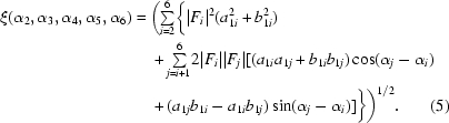
C_N is the Hermitian covariance matrix of the N-dimensional Gaussian probability distribution and z_ij denotes the ijth element of the inverse matrix of C_N. After separately summing over the diagonal and off-diagonal terms, transformation to polar coordinates and simplification, we obtain

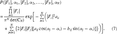In the above equation, a_ij and b_ij represent the real and imaginary components of the inverse covariance matrix. The unknown phase angles α₁, α₂, α₃ need to be integrated out.

The inner integral can be solved analytically:

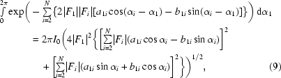where I ₀(x) is the zero-order modified Bessel function of the first kind.

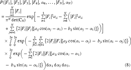
From the definition of conditional probability, the required probability distribution can be obtained as follows,

P(|F ₁|, |F ₂|, |F ₃|, |F ₄|, α₄, …, |F_N|, α_N) is given by (8) and (9) and P(|F ₄|, α₄, …, |F_N|, α_N) can be obtained by (7), denoting the corresponding covariance matrix by C_N−3 and the ijth element of its inverse by c_ij + id_ij. Thus, the required distribution is

where

Appendix B. The covariance matrix

In order to take into account all the correlations between the three observations and three models, a 6 × 6 covariance matrix must be constructed:

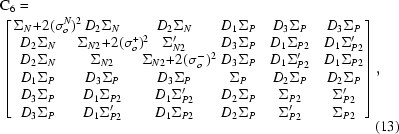with the model part covariance matrix C₃ being the right bottom 3 × 3 submatrix of (13),

where D is a refinable Luzzati (1952 ▶) error parameter which absorbs the errors in both model phases and amplitudes: the D ₁ parameter accounts for the errors between the observed and calculated phases and amplitudes, the D ₂ error parameter accounts for the errors between the native and derivative structure factors caused by non-isomorphism and D ₃ accounts for the combination of these errors. In general, the covariance term Σ′_N2 is complex; however, the imaginary term is small compared with the real term for a large number of reflections and is thus omitted. Furthermore, the real part of this term is a function of the difference between ‘observed’ phases which are unknown and is approximated by the difference between the model phases. The following covariance-matrix terms arise,

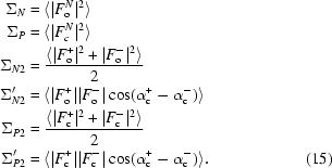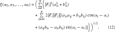
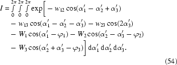
Appendix C. Properties of the three-dimensional SIRAS integral

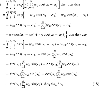
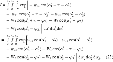
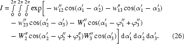
Let us consider the integral and its properties before the analytical integration is performed. From (8), after dis­regarding the anomalous terms (see Appendix B ), the integral is as follows:

For simplicity, let us define the w_ij term as

then after expanding the integrand by using the trigonometric relations and rearranging the terms we obtain

If we now define vectors W _i, i = 1, 2, 3, by

and denote their modulus and polar angle by W_i and ϕ_i, respectively, then

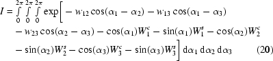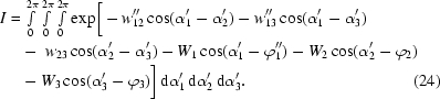
and we obtain the simplified form of the integral with the integrand consisting of only six terms:

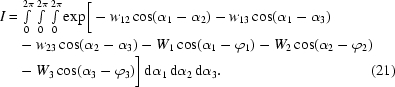Thus, the integral depends on nine real-number parameters: the w parameters W ₁, W ₂, W ₃, w ₁₂, w ₁₃, w ₂₃ and phases ϕ₁, ϕ₂, ϕ₃, so we can look at it as a function of nine real variables I = I(W ₁, W ₂, W ₃, w ₁₂, w ₁₃, w ₂₃, ϕ₁, ϕ₂, ϕ₃) (in the following, the set of nine variables will be denoted as an ennead). We can now reduce the range of the definition of this function.

Let the ennead ≡ (W ₁, W ₂, W ₃, w ₁₂, w ₁₃, w ₂₃, ϕ₁, ϕ₂, ϕ₃) be I-equivalent to ennead (W′₁, W′₂, W′₃, w′₁₂, w′₁₃, w′₂₃, ϕ′₁, ϕ′₂, ϕ′₃) if I(W ₁, W ₂, W ₃, w ₁₂, w ₁₃, w ₂₃, ϕ₁, ϕ₂, ϕ₃) is the same as I(W′₁, W′₂, W′₃, w′₁₂, w′₁₃, w′₂₃, ϕ′₁, ϕ′₂, ϕ′₃).

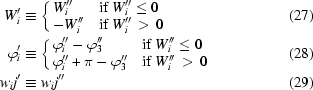
Furthermore, define w_ab as w-least in if |w_ab| ≤ |w ₁₂|, |w_ab| ≤ |w ₁₃| and |w_ab| ≤ |w ₂₃|.

The following statement holds.

Statement

For any ennead ≡ (W ₁, W ₂, W ₃, w ₁₂, w ₁₃, w ₂₃, ϕ₁, ϕ₂, ϕ₃) an ennead ≡ (W′₁, W′₂, W′₃, w′₁₂, w′₁₃, w′₂₃, ϕ′₁, ϕ′₂, 0) exists which is I-equivalent with and for which all W ₁′, W ₂′, W ₃′ are nonpositive and all w′₁₂, w′₁₃, w′₂₃ up to the w-least in are nonpositive.

Proof

We will construct in two steps. At first, let us construct ≡ (W′′₁, W′′₂, W′′₃, w′′₁₂, w′′₁₃, w′′₂₃, ϕ′′₁, ϕ′′₂, ϕ′′₃) I-­equivalent with for which all w′′₁₂, w′′₁₃, w′′₂₃ up to the w-least in are nonpositive. Four distinct cases can occur:

• (i) All w ₁₂, w ₁₃, w ₂₃ are nonpositive. Then, trivially, = .

• (ii) Exactly one of w ₁₂, w ₁₃, w ₂₃ is positive. If w-least in is positive, = . Let us assume that the only positive parameter is not w-least in . 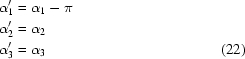Because of the formal symmetry of I with regards to indices 1, 2, 3, we can freely choose w ₁₂ to be positive and w ₁₃ to be (nonpositive) w-least in without the loss of generality (the proof would be symbolically the same for any other permutation of positive and -least variables). We perform the following linear transformation of the integral from (α₁, α₂, α₃) to (α′₁, α′₂, α′₃),

  

  

  If we now set w′′₁₂ ≡ −w ₁₂, w′′₁₃ ≡ −w ₁₃, ϕ′′₁ ≡ ϕ₁ − π then

  

  Thus, = (W′′₁, W′′₂, W′′₃, w ₁₂′′, w ₁₃′′, w ₂₃′′, ϕ′′₁, ϕ′′₂, ϕ′′₃) = (W ₁, W ₂, W ₃, −w ₁₂, −w ₁₃, w ₂₃, ϕ₁ − π, ϕ₂, ϕ₃) is I-equivalent with , w′′₁₃ is the w-least in and both w′′₁₂, w′′₂₃ are nonpositive.

• (iii) Exactly two of w ₁₂, w ₁₃, w ₂₃ are positive. Again, we can freely choose w ₁₂ and w ₁₃ to be positive and the proof would be symbolically the same for any other choice. The linear transformation (22) shows that = (W ₁, W ₂, W ₃, −w ₁₂, −w ₁₃, w ₂₃, ϕ₁ − π, ϕ₂, ϕ₃) is I-equivalent with and all w′′₁₂, w′′₁₃, w′′₂₃ are nonpositive.

• (iv) All w ₁₂, w ₁₃, w ₂₃ are positive. If we choose w ₂₃ to be w-­least in , then again the transformation (22) ensures that = (W ₁, W ₂, W ₃, −w ₁₂, −w ₁₃, w ₂₃, ϕ₁ − π, ϕ₂, ϕ₃) is I-­equivalent with , w ₂₃′′ is w-least in and w′′₁₂, w′′₁₃ are nonpositive.

Now will be constructed from . The transformation

turns I() into

We define = (W′₁, W′₂, W′₃, w′₁₂, w′₁₃, w′₂₃, ϕ′₁, ϕ′₂, ϕ′₃) by

Now the I-equivalency of with is shown for the case of all W′′₁, W′′₂, W′′₃ being nonpositive and the following property of the cos() function

shows that is also I-equivalent with for any positive W′′_i. Since is I-equivalent with and I-equivalency is transitive by definition, we obtain that is I-equivalent with . Clearly, all W′₁, W′₂, W′₃, w′₁₂, w′₁₃, w′₂₃ up to w-least in are nonpositive.

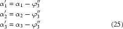
Since the proof is constructive, it provides a way of transforming any integral I() coming from real data to I(), reducing the definition range of I. Because ϕ′₃ is fixed (zero), we could reduce the ennead into an octad. However, this would break the formal symmetry of I, causing several formulae to become slightly more complicated. Therefore, the ennead form will be used throughout. For simplicity, the primes will be omitted and will be used instead of .

Appendix D. Integrand maximum localization

The following statement provides partial localization of the maximum position if certain conditions hold for .

Statement

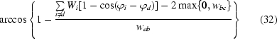
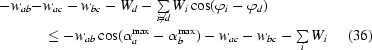
Let us have the function F(α_a, α_b, α_c) ≡ exp[−w_abcos(α_a − α_b) − w_accos(α_a − α_c) − w_bccos(α_b − α_c) − W_dcos(α_d − ϕ_d) − W_ecos(α_e − ϕ_e) − W_fcos(α_f − ϕ_f)], where {a, b, c} = {d, e, f} = {1, 2, 3}, |w_ab| = max|w_ij| > 0, |w_bc| = min|w_ij|, |W_d| = max|W_i| and all W_d, W_e, W_f, w_ab, w_ac are nonpositive. If

then the maximum of F is at most

distant from the plane α_a = α_b in the three-dimensional Cartesian coordinate system with axes α_a, α_b, α_c.

Proof

Since the exponential function (exp) is an increasing function, it is sufficient to prove the statement for the function F′(α_a, α_b, α_c) ≡ −w_abcos(α_a − α_b) − w_accos(α_a − α_c) − w_bccos(α_b − α_c) − W_dcos(α_d − ϕ_d) − W_ecos(α_e − ϕ_e) − W_fcos(α_f − ϕ_f). Let us discuss the case when w_bc ≤ 0 first. We need to show that

Clearly,

Take the function value at point (ϕ_d, ϕ_d, ϕ_d):

Since F′(ϕ_d, ϕ_d, ϕ_d) ≤ F(α_a ^max, α_b ^max, α_c ^max) from (34) and (35) we obtain

leading to

From the assumptions, 0 ≤ 1 − { W_i[1 − cos(ϕ_i − ϕ_d)]}/w _ab ≤ 1; therefore, the arccosine of this expression is always well defined and (33) holds.

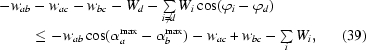
Let w_bc > 0. Then

which together with (35) means that

The assumptions assure that 0 ≤ 1 − { W_i[1 − cos(ϕ_i − ϕ_d)] − 2w_bc}/w _ab ≤ 1, thus

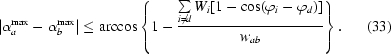
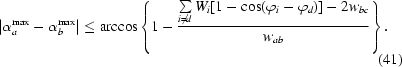
In Appendix C , we have shown that the validity of all the assumptions of the sentence except of the crucial assumption (31), which is equivalent to

The larger the difference, the better the localization of the maximum. Now the question arises: what are the typical values of this difference in the case of protein SIRAS data? Typically, the structure-factor contributions of heavy atoms are much smaller than the contributions from protein atoms, F ₁ ≃ F ₂ ≃ F ₃ and α₄ ≃ α₅ ≃ α₆. From F ₁ ≃ F ₂ ≃ F ₃ and definition (17),

where k is constant for all w_ij in this broad approximation. Furthermore, from α₄ ≃ α₅ ≃ α₆ and definition (19),

Let us now take the definition of the covariance matrix for the SIRAS function C₆ from (13) which must be positive definite. Using the analytical solution of the inverse of the covariance matrix, it can be shown that

where

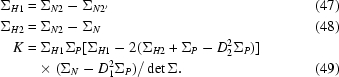Usually, 0 < D_i < 1, which means that

Furthermore, the real part of the atomic scattering factor f + f′ of a heavy atom is typically much larger than its imaginary part f′′ and subsequently Σ_H2 ≃ f_i + f _i′ Σ_H1 ≃ 2f _i′′. Since it can be proven that (Σ_N − D ₁ ²Σ_P) > 0 from the positive definiteness of Σ, we obtain

and because of (50) also

meaning that |a ₂₃| a ₂₄ + a ₂₅ + a ₂₆|, |a ₂₃| a ₃₄ + a ₃₅ + a ₃₆| and subsequently |w ₂₃| |W ₂|, |w ₂₃| |W ₃| according to (43) and (44). This means that in a typical case |w _ab| | W_i[1 − cos(ϕ_i − ϕ_d)]| and therefore the assumption (31) of the previous sentence should be fulfilled for typical SIRAS reflections. Indeed, the statistics from several SIRAS data sets shows that (31) is valid for the vast majority (over 99%) of reflections.

Appendix E. The SIRAS integral evaluation algorithm

Let us assume that the a and b indices from the Appendix D statement are equal to 2 and 3, respectively, i.e. the maximum lies close to the plane α₂ = α₂ (we have shown that the typical values of these indices are 2 and 3 later in Appendix D ). Let us rotate the coordinate system (α₁, α₂, α₃) to (α′₁, α′₂, α′₃) so that the plane α₂ = α₃ is equivalent to the plane given by coordinate axes α′₁, α′₂. The following transformation can be used,

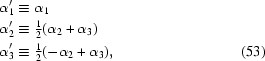transforming the integral I(α₁, α₂, α₃) to

The maximum is now close to the plane given by axes α′₁, α′₂ and sampling of the variable α′₂ over a short range around 0 in the numerical integration is sufficient to cover the peak. The largest required range can be estimated from the maximal distance of the maximum to the plane given by expression (32).

Based on the previous results and discussions, the following algorithm was implemented in REFMAC5 for the SIRAS function integral (and its first and second derivatives) calculation.

• (i) The ennead is calculated using definitions (17) and (19) and, if required, transformations (22) and (25) are applied so that all the w parameters up to the w-least in are nonpositive.

• (ii) The upper limit of the maximum peak height (let us denote it by ζ) is calculated as the sum of the absolute values of all w parameters. If this value is larger than a given threshold and |w_ab| is larger than a given threshold, the reflection is classified into class A, otherwise into class B. The reflections in class A can be expected to give rise to larger peaks while the function I(α₁, α₂, α₃) is considered to be flat for class B reflections.

• (iii) If the reflection belongs to class A, then the validity of assumption (31) is verified. If the assumption holds, the reflection is classified into class A1 and otherwise into class A2.

• (iv) If the reflection belongs either to class B or to class A2 then the required sampling of both integration variables is estimated according to the value of ζ (the higher ζ, the denser the sampling) and numerical integration is performed according to (4), without the transformation (53) of the function and over the whole integration area.

• (v) If the reflection belongs to class A1, the transformation (53) is performed. The variable α′₃ is only sampled over a short range around 0. If the maximal peak-to-plane distance (32) is shorter than a given threshold, the approximation α₂ ≃ α₃ may be used, leading to a better estimation of ζ and hence a better sampling estimate.

References

- Abrahams, J. P. & Leslie, A. G. W. (1996). Acta Cryst. D52, 30–42. [DOI] [PubMed]
- Badger, J. (2003). Acta Cryst. D59, 823–827. [DOI] [PubMed]
- Beck, T., Krasauskas, A., Gruene, T. & Sheldrick, G. M. (2008). Acta Cryst. D64, 1179–1182. [DOI] [PubMed]
- Berman, H. M., Westbrook, J., Feng, Z., Gilliland, G., Bhat, T. N., Weissig, H., Shindyalov, I. N. & Bourne, P. E. (2000). Nucleic Acids Res.28, 235–242. [DOI] [PMC free article] [PubMed]
- Boggon, T. J. & Shapiro, L. (2000). Structure, 8, R143–R149. [DOI] [PubMed]
- Bricogne, G. & Irwin, J. (1996). Proceedings of the CCP4 Study Weekend. Macromolecular Refinement, edited by E. J. Dodson, M. Moore, A. Ralph & S. Bailey, pp. 85–92. Warrington: Daresbury Laboratory.
- Collaborative Computational Project, Number 4 (1994). Acta Cryst. D50, 760–763.
- Cowtan, K. (1999). Acta Cryst. D55, 1555–1567. [DOI] [PubMed]
- Dauter, Z., Dauter, M. & Rajashankar, K. R. (2000). Acta Cryst. D56, 232–237. [DOI] [PubMed]
- Dauter, Z., Li, M. & Wlodawer, A. (2001). Acta Cryst. D57, 239–249. [DOI] [PubMed]
- DeLaBarre, B. & Brunger, A. T. (2006). Acta Cryst. D62, 923–932. [DOI] [PubMed]
- Graaff, R. A. G. de, Hilge, M., van der Plas, J. L. & Abrahams, J. P. (2001). Acta Cryst. D57, 1857–1862. [DOI] [PubMed]
- La Fortelle, E. de & Bricogne, G. (1997). Methods Enzymol.276, 472–494. [DOI] [PubMed]
- Long, F., Vagin, A. A., Young, P. & Murshudov, G. N. (2008). Acta Cryst. D64, 125–132. [DOI] [PMC free article] [PubMed]
- Grosse-Kunstleve, R. W., Sauter, N. K., Moriarty, N. W. & Adams, P. D. (2002). J. Appl. Cryst.35, 126–136.
- Luzzati, V. (1952). Acta Cryst.5, 802–810.
- Matthews, B. W. (1966). Acta Cryst.20, 82–86.
- Murshudov, G. N., Vagin, A. A. & Dodson, E. J. (1997). Acta Cryst. D53, 240–255. [DOI] [PubMed]
- Ness, S. R., de Graaff, R. A. G., Abrahams, J. P. & Pannu, N. S. (2004). Structure, 12, 1753–1761. [DOI] [PubMed]
- North, A. C. T. (1965). Acta Cryst.18, 212–216.
- Pannu, N. S., McCoy, A. J. & Read, R. J. (2003). Acta Cryst. D59, 1801–1808. [DOI] [PubMed]
- Pannu, N. S., Murshudov, G. N., Dodson, E. J. & Read, R. J. (1998). Acta Cryst. D54, 1285–1294. [DOI] [PubMed]
- Pannu, N. S. & Read, R. J. (1996). Acta Cryst. A52, 659–668.
- Pannu, N. S. & Read, R. J. (2004). Acta Cryst. D60, 22–27. [DOI] [PubMed]
- Perrakis, A., Morris, R. & Lamzin, V. S. (1999). Nature Struct. Biol.6, 458–463. [DOI] [PubMed]
- Sheldrick, G. M. (2008). Acta Cryst. A64, 112–122. [DOI] [PubMed]
- Skubák, P., Murshudov, G. N. & Pannu, N. S. (2004). Acta Cryst. D60, 2196–2201. [DOI] [PubMed]
- Skubák, P., Ness, S. & Pannu, N. S. (2005). Acta Cryst. D61, 1626–1635. [DOI] [PubMed]
- Sun, S., Kondabagil, K., Gentz, P. M., Rossmann, M. G. & Rao, V. B. (2007). Mol. Cell, 25, 943–949. [DOI] [PubMed]
- Szczepanowski, R. H., Filipek, R. & Bochtler, M. (2005). J. Biol. Chem.280, 22006–22011. [DOI] [PubMed]
- Taylor, G. (2003). Acta Cryst. D59, 1881–1890. [DOI] [PubMed]
- Wernimont, A. K., Huffman, D. L., Lamb, A. L., O’Halloran, T. V. & Rosenzweig, A. C. (2000). Nature Struct. Biol.7, 766–771. [DOI] [PubMed]