ELECTRODYNAMIC CONSTRAINTS ON HOMOGENEITY AND RF POWER DEPOSITION IN MULTIPLE COIL EXCITATIONS

Abstract

The promise of increased SNR and spatial/spectral resolution continues to drive MR technology toward higher magnetic field strengths. SAR management and B₁ inhomogeneity correction become critical issues at the high frequencies associated with high field MR. In recent years, multiple coil excitation techniques have been recognized as potentially powerful tools for controlling SAR while simultaneously compensating for B₁ inhomogeneities. This work explores electrodynamic constraints on transmit homogeneity and SAR, for both fully parallel transmission and its time-independent special case known as RF shimming. Ultimate intrinsic SAR – the lowest possible SAR consistent with electrodynamics for a particular excitation profile but independent of transmit coil design – is studied for different field strengths, object sizes and pulse acceleration factors. The approach to the ultimate intrinsic limit with increasing numbers of finite transmit coils is also studied, and the tradeoff between homogeneity and SAR is explored for various excitation strategies. In the case of fully parallel transmission, ultimate intrinsic SAR shows flattening or slight reduction with increasing field strength, in contradiction to the traditionally cited quadratic dependency, but consistent with established electrodynamic principles.

INTRODUCTION

The advantages of using high magnetic field strengths for MR imaging and spectroscopy are well known: they include the promise of improved signal-to-noise ratio (SNR) and spatial or spectral resolution, as well as the potential for improvements in certain useful forms of contrast. The challenges of high field strength are also well known, including a variety of difficulties associated with reduced homogeneity in both static and radiofrequency (RF) fields. For RF fields in particular, the operating wavelength decreases as field strength and Larmor frequency increase, becoming ever smaller as compared to the dimensions of the human body, and resulting in ever larger interactions between electromagnetic fields and dielectric tissues. These interactions lead to local focusing of the RF magnetic field B₁, both in excitation and in reception. The focusing of B₁ field results in interference patterns (1), which compromise the underlying SNR increases associated with high field strength and which would in many cases markedly impede clinical diagnosis. B₁ focusing also results in subject-specific spatial variations of flip angle, which can diminish the reliability of image contrast. Meanwhile, the focusing of RF electric fields in dielectric tissues at high frequency results in increasingly inhomogeneous and subject-dependent specific absorption rate (SAR). Furthermore, the magnitude of electric fields produced for a given strength of the transmit magnetic field (i.e. per unit flip angle of RF excitation) is generally expected to grow with frequency. These electric fields induce eddy currents and dissipate heat in the body, causing an overall SAR increase which has (in admittedly casual approximations based on low- to moderate-frequency behavior) been taken to increase approximately with the square of the frequency.

Compensation of B₁ inhomogeneities and management of SAR are indeed among the most difficult challenges faced by in-vivo ultra high field MR applications. RF-induced heating is a potentially elevated safety concern at high field strength, both requiring careful design and evaluation of RF coils and necessitating worst-case safety limits on flip angles in MR pulse sequences, which can further erode achievable high-field SNR and contrast. Various approaches to homogeneity correction and SAR management have been proposed, involving either coil design or pulse sequence design.

At low magnetic field strength, birdcage coils are commonly used to produce homogeneous excitations over a large fields of view, but traditional birdcage designs can exhibit significant B₁ inhomogeneities and SAR increases when operating at high frequency (2). Various novel volume coil designs with improved homogeneity and efficiency at high field strength have been developed in recent years (3,4). Recent work using numerical methods has also shown that further variations in RF coil design can serve to redistribute RF energy absorption over the imaged object, in order to remove hot spots caused by RF field concentrations (5).

One noteworthy feature which has begun to distinguish high-field coil design is the use of multiple transmit elements or drive points. This provides additional degrees of freedom which may be used to control the distribution of electromagnetic fields. In particular, independent control of the driving amplitude and phase of individual current elements can be effective in correcting B₁ inhomogeneities – an approach generally referred to as RF shimming (4,6–9). RF shimming has been shown to be effective in improving B₁ homogeneity at high magnetic fields when an adequate number of coils is available (10). A recent study showed that SAR reduction may be achieved together with improved B₁ uniformity by optimizing the amplitudes and phases of the elements of a transmit array (11).

RF power deposition and B₁ homogeneity can also be controlled to some extent by pulse or pulse sequence design, for example using SAR-optimized flip angles (12), or variable-rate selective excitations (VERSE) (13). Hennig et al. have reported substantial SAR reductions in spin echo sequences using hyperecho techniques (14). Composite pulses have been used successfully with single coils (15) and coil arrays (16) to improve excitation homogeneity, and array-optimized composite pulse design can be also pursued for reducing local SAR levels (16). Parallel MRI techniques (17–19) may be used to decrease the number and frequency of RF excitations, thereby reducing total RF power deposition, albeit at the expense of signal to noise ratio (SNR).

Recently, parallel transmit MR techniques (20,21) – which combine multi-coil excitation and pulse design – have been explored with increasing interest. These techniques, which are generalizations of RF shimming with the additional capability to perform B₁ optimization in the time domain, were originally designed to accelerate complex excitation pulses, by analogy with the principles underlying parallel MRI. By driving each element of an array of transmit coils with a distinct tailored RF waveform, parallel excitation techniques enable the suppression of aliasing lobes resulting from reduction of the sampling density in excitation k-space. In these approaches, the composite B₁ field is modulated in space and time by adjusting the independent RF waveforms transmitted by each coil, and is combined with a suitable synchronous gradient waveform in order to generate a target excitation profile.

Early in the development of parallel transmit MR, it was also recognized that parallel transmission can be exploited to improve the homogeneity of RF excitations and to reduce SAR (21). These capabilities account in part for the great recent interest in parallel transmission as an enabling technology for high-field MRI. It should be noted, however, that the demands of pulse acceleration and the demands of SAR reduction may often be opposed, since calculation of the weights required to produce an accelerated excitation relies on the inversion of ill-conditioned sensitivity matrices, which may cause spatial amplification of SAR somewhat analogous to the spatial amplification of noise in parallel imaging (22). Also by analogy with the case of parallel reception, it is possible to derive a set of transmit coil waveforms which yield the minimum SAR for a given level of pulse acceleration (21).

Parallel transmission methods require prior knowledge of B₁ field distributions, as well as hardware capable of generating and amplifying multiple independent RF waveforms. In order to justify these additional investments in calibration and technology, it will be important to assess how well fully parallel transmission can perform. Katscher et al. have shown that suboptimal coil arrays may have a negligible effect on the quality of the excitation pattern in fully parallel transmission, whereas they dramatically affect SAR, even for slight variations in the spatial arrangement of individual elements (23). This result also suggests that it will be important to assess the tradeoff between excitation fidelity or homogeneity and SAR. In this paper, we present a framework in which the homogeneity and SAR associated with various transmission approaches may be compared independent of any particular coil configuration. We also present a lower bound on SAR as a guide for future transmit coil array designs.

In the case of parallel imaging it has been shown that there is an inherent electrodynamic limitation to the achievable SNR of any physically realizable coil array, and the behavior of ultimate intrinsic SNR has been extensively studied (24–26). In those prior studies, receive coil sensitivities were expanded in a complete basis of valid solutions to Maxwell’s equations and the optimal SNR was calculated by finding a linear combination that minimized the total noise power for unit signal strength. In this paper we use a similar approach to explore electrodynamic constraints on transmit homogeneity and SAR, by expanding putative transmit coil fields in a suitable basis to compute the ultimate intrinsic SAR for various excitation approaches. We explore the dependency of ultimate intrinsic SAR upon field strength and investigate the effects of varying the shape of the target excitation as well as the size of the imaged body (since wavelength effects can be strongly influenced by object size). In addition, we model the same excitation approaches using finite coil arrays of well-defined geometry, and compare their performance against the ultimate intrinsic case. In the case of fully parallel excitation, we investigate the relation between ultimate SAR and acceleration factor, and we determine the time-varying spatial distribution of RF power deposition within the subject during optimized excitation pulses.

THEORY

In this section we begin by reviewing the general formalism of excitation with an array of transmit coils and then we describe a procedure for combining the individual coils’ current waveforms in order to minimize RF power deposition in the subject while preserving a target net excitation profile. We then show a method to derive a theoretical lower bound on this deposited power, by employing a complete basis set of transmit coil fields.

Multi-coil RF excitation formalism

It is often convenient to express the RF field generated by a transmit coil in a reference frame rotating at angular frequency equal to the Larmor frequency, as in this way the carrier term exp(i t) disappears from the equations. The principle of reciprocity, commonly used to calculate the strength of the MR signal, must be adapted accordingly. A rigorous formulation was provided by Hoult (27), who derived the following expressions for the magnetic field in the positively and negatively rotating frame, as a function of the components of the magnetic field in the static laboratory frame:

$$\begin{array}{l}{\stackrel{\sim }{\mathit{B}}}_1^{+}=\frac{{\mathit{B}}_{1,x}+\mathit{i}{\mathit{B}}_{1,y}}{2}\\ {\stackrel{\sim }{\mathit{B}}}_1^{-}=\frac{{({\mathit{B}}_{1,x}-\mathit{i}{\mathit{B}}_{1,y})}^{\ast }}{2},\end{array}$$ [1]

where * indicates complex conjugation and ℬ_1,x and ℬ_1,y are the Cartesian components of the complex RF field amplitude generated by a coil in the laboratory frame (with the carrier terms removed). The RF excitation may be expressed in terms of ${\stackrel{\sim }{\mathit{B}}}_1^{+}$, whereas, in accordance with the principle of reciprocity, the strength of the received MR signal is proportional to ${\stackrel{\sim }{\mathit{B}}}_1^{-}$. Neglecting short-lived field transients and assuming a driven steady state which changes slowly as compared with the RF oscillation period, ${\stackrel{\sim }{\mathit{B}}}_1^{+}$ can be separated into a spatially varying term and a temporal envelope:

$${\stackrel{\sim }{\mathit{B}}}_1^{+}(\mathbf{r},t)=b(\mathbf{r})\text{I}(t)$$ [2]

It is important to remember that both factors on the right hand side of Eq. [2] are complex quantities: b(r) because of its orientation in the positively rotating frame and I(t) because it is an oscillatory current which has a magnitude and a phase in time.

Let us now consider an array of transmit coils. Within the limits of the small tip-angle approximation, the transverse magnetization resulting from simultaneous excitation with L transmit coils can be derived using k-space Fourier analysis (21):

$$M(\mathbf{r})=i\gamma M_{\text{O}}(\mathbf{r})\sum _{l^{\prime }=1}^L{b}_{l^{\prime }}(\mathbf{r})\underset{k}{\int }\sum _{l=1}^L{c}_{l^{\prime },l}{W}_l(\mathbf{k})S(\mathbf{k})e^{i2\pi \mathbf{k}·\mathbf{r}}\text{d}\mathbf{k}.$$ [3]

γ is the gyromagnetic ratio, i is the imaginary unit, M_O is the equilibrium value of the nuclear magnetization, b_l(r) is the complex spatial weighting induced by the ${\stackrel{\sim }{\mathit{B}}}_1^{+}$ field pattern of the l^th component coil in the array, and c_l′,l are the coefficients that characterize the mutual coupling between the coils. In practice, rather than b_l′(r), it is convenient to measure, by means of so-called B₁ maps, the effective spatial weighting ${\widehat{b}}_l(\mathbf{r})={\sum }_{l^{\prime }=1}^L{c}_{l^{\prime },l}{b}_{l^{\prime }}(\mathbf{r})$, which incorporates the mutual coupling. The product of the spatial-frequency weighting introduced by the l^th coil, W_l(k), and the excitation k-space sampling trajectory controlled by the switching gradients, S(k), represents the explicit weighting of k-space by the RF excitation and is defined as (28):

$$W_l(\mathbf{k})S(\mathbf{k})=\underset{0}{\overset{T}{\int }}{W}_l(\mathbf{k}(t))\left\{{}^3\delta (\mathbf{k}(t)-\mathbf{k})\mid \stackrel{.}{\mathbf{k}}(t)\mid \right\}dt=\underset{0}{\overset{T}{\int }}\frac{{\text{I}}_l(t)}{\mid \gamma \mathbf{G}(t)\mid }\left\{{}^3\delta (\mathbf{k}(t)-\mathbf{k})\mid \stackrel{.}{\mathbf{k}}(t)\mid \right\}dt,$$ [4]

where |G(t)| is the amplitude of the linear gradients and ³δ the three-dimensional delta function. I_l(t) is the current circulating in the l^th coil and it is a measure of the amplitude of the RF field applied by the l^th coil to produce an ideal small tip-angle excitation at the voxel of interest in the current RF cycle.

The portion of Eq. [3] that defines the complex-valued excitation profile μ(r) can thus be re-written as:

$$\mu (\mathbf{r})=\sum _{l=1}^L{\widehat{b}}_l(\mathbf{r})\underset{k}{\int }{W}_l(\mathbf{k})S(\mathbf{k})e^{i2\pi \mathbf{k}·\mathbf{r}}\text{d}\mathbf{k}$$ [5]

Let us now consider the case of a 2D echo-planar excitation trajectory. Indicating positions on the trajectory with (k_x, k_y), we can define the periodic excitation pattern f_l(x, y) associated with the RF pulse of the l^th transmit element as:

$$f_l(x,y)=\underset{k_x,k_y}{\iint }{W}_l(k_x,k_y)e^{i2\pi (k_{x}x+k_{y}y)}\text{d}{k}_x\text{d}{k}_y$$ [6]

(Note that, as compared with the original exposition in Ref. (21), we have changed notation for the excitation pattern from g to f so as to avoid confusion with the g-factor in parallel imaging). The periodic patterns are then combined to excite simultaneously the target profile. This translates into the following constraint for the f_l(x, y)’s in Eq. [6]:

$$\sum _{l=1}^L{f}_l(x,y){\widehat{b}}_l(x,y)=\mu (x,y)$$ [7]

From Eq. [6] is clear that discrete sampling in the spatial-frequency domain (k_x, k_y) results in aliasing lobes in the x and y directions. If the sampling interval is sufficiently small, all the aliasing lobes occur outside the FOV and we need not include the periodicity of the f_l(x, y) explicitly in the equation. This is the case for unaccelerated parallel transmission, which requires solving Eq. [7] for each voxel in the image separately.

RF power deposition with multiple transmit coils

The total electric field associated with the pth time-period in the RF excitation can be expressed as a linear combination of the electric fields generated by the L elements of the transmit array:

$$\mathit{E}(\mathbf{r},p\mathrm{\Delta }t)=\sum _{l=1}^L{\mathbf{I}}_l(p\mathrm{\Delta }t){\mathbf{e}}_l(\mathbf{r}),$$ [8]

where I_l(pΔt) is the p-th complex-valued time-sample of the current applied for an interval Δt to the l^th transmit element or driving port, and e_l(r) denotes the complex-valued electric field which would be produced by the l^th coil if I_l(pΔt) were equal to 1. The temporal window Δt is assumed small enough that the field amplitudes can be considered constant within it. The RF power dissipated in the subject over one excitation time period can be expressed as a quadratic function in the samples of the current waveforms:

$$\begin{array}{l}{\xi }_p=\frac{1}{2}\underset{V}{\int }\underset{\mathrm{\Delta }t}{\int }\sigma (\mathbf{r})\mid \mathit{E}(\mathbf{r},p\mathrm{\Delta }t){\mid }^2\mathit{dtdv}\\ ={({\text{I}}_1(p\mathrm{\Delta }t)\mathrm{..}{\text{I}}_l(p\mathrm{\Delta }t)\mathrm{..}{\text{I}}_L(p\mathrm{\Delta }t))}^H\left(\frac{\mathrm{\Delta }t}{2}\underset{V}{\int }\sigma (\mathbf{r}){\left(\begin{array}{c}{\mathbf{e}}_1(\mathbf{r})\\ \stackrel{·}{{\mathbf{e}}_l(\mathbf{r})}\\ \stackrel{·}{{\mathbf{e}}_L(\mathbf{r})}\end{array}\right)}^{\ast }\underset{·}{\overset{·}{({\mathbf{e}}_1(\mathbf{r})\mathrm{..}{\mathbf{e}}_l(\mathbf{r})}}\underset{·}{\overset{·}{\mathrm{..}{\mathbf{e}}_L(\mathbf{r}))}}dv\right)\left(\begin{array}{c}{\text{I}}_1(p\mathrm{\Delta }t)\\ \dots \\ {\text{I}}_l(p\mathrm{\Delta }t)\\ \dots \\ {\text{I}}_L(p\mathrm{\Delta }t)\end{array}\right)\\ ={\mathbf{I}}_p^H\mathbf{\Phi }{\mathbf{I}}_p\end{array}$$ [9]

σ(r) is the conductivity of the sample, and the superscripts ^* and ^H denote, respectively, complex conjugate and conjugate (Hermitian) transpose. Φ is a matrix which contains the overlap integrals of the electric fields from the individual coils and its elements are calculated as:

$${\mathbf{\Phi }}_{l,l^{\prime }}=\underset{V}{\int }\sigma (\mathbf{r}){\mathbf{e}}_l(\mathbf{r})·{\mathbf{e}}_{l^{\prime }}^{\ast }(\mathbf{r})dv$$ [10]

(Note that Eq. [10] is equivalent, by reciprocity, to the expression for the noise correlation matrix between transmit elements if they were used in receive mode.) The samples of the current waveforms (I_l(pΔt)) are related by Fourier transformation to the periodic patterns that define the excitation profile (see Eq. [4] and [6]):

$$W_{lp}\equiv W_l(k_x,k_y)=W_l(\mathbf{k}(p\mathrm{\Delta }t))=\frac{{\text{I}}_l(p\mathrm{\Delta }t)}{\mid \gamma \mathbf{G}(p\mathrm{\Delta }t)\mid }\Rightarrow f_{ln}\equiv f_1(x,y)=F\left[W_{lp}\right]\propto F[{\text{I}}_l(p\mathrm{\Delta }t)]$$ [11]

where ℱ indicates the Fourier transform, and n is an index of discrete voxel positions (x, y) considered in defining the excitation profile. The factor |γG(pΔt) has been absorbed into the proportionality on the right hand side of Eq. [11], as it remains constant for the EPI trajectory in question. Eq. [11] explicitly shows how time dependence disappears from the remainder of the theory and becomes incorporated in the index p. The notation used here in fact indicates that, for each time period p, time-variant quantities are sampled only at time points corresponding to positions (k_x, k_y) lying on the excitation k-space trajectory. The mapping of k-space positions to spatial voxel locations by Fourier transformation applies also to the corresponding indices (p and n), as follows:

$$\begin{array}{ccc}(k_x,k_y)& \to & p\\ {\Updownarrow }_F& & {\Updownarrow }_F\\ (x,y)& \to & n\end{array}$$ [12]

Because of the property detailed in Eq. [11], we can apply Parseval’s theorem to write RF power deposition using the f_ln’s:

$$\begin{array}{c}\sum _{p=1}^P{\mathbf{I}}_p^H\mathbf{\Phi }{\mathbf{I}}_p=\sum _{p=1}^P\sum _{l=1}^L\sum _{l^{\prime }=1}^L{\text{I}}_{l^{\prime }}^{\ast }(p\mathrm{\Delta }t){\mathrm{\Phi }}_{l^{\prime },l}{\text{I}}_l(p\mathrm{\Delta }t)=\sum _{l=1}^L\sum _{l^{\prime }=1}^L{\mathrm{\Phi }}_{l^{\prime },l}\left(\sum _{p=1}^P{\text{I}}_{l^{\prime }}^{\ast }(p\mathrm{\Delta }t){\text{I}}_t(p\mathrm{\Delta }t)\right)\propto \\ \sum _{l=1}^L\sum _{l^{\prime }=1}^L{\mathrm{\Phi }}_{l^{\prime },l}\left(\sum _{n=1}^N{f}_{l^{\prime }n}^{\ast }{f}_{ln}\right)=\sum _{n=1}^N\sum _{l=1}^L\sum _{l^{\prime }=1}^L{f}_{l^{\prime }n}^{\ast }{\mathrm{\Phi }}_{l^{\prime },l}{f}_{ln}=\sum _{n=1}^N{\mathbf{f}}_n^H\mathbf{\Phi }{\mathbf{f}}_n,\end{array}$$ [13]

where P is the total number of time periods in the excitation and N is the total number of voxels. Using the result of Eq. [13] in Eq. [9], we can define the average RF power deposited in the sample during the excitation with two equivalent expressions:

$$\xi =\frac{1}{P}\sum _{p=1}^P{\mathbf{I}}_p^H\mathbf{\Phi }{\mathbf{I}}_p=\frac{1}{N}\sum _{n=1}^N{\mathbf{f}}_n^H\mathbf{\Phi }{\mathbf{f}}_n.$$ [14]

Optimal RF power deposition with fully parallel transmission

In fully parallel transmission tailored excitations are transmitted independently with the individual array elements. This means that each coil’s base excitation pattern may vary independently voxel-by-voxel, since that coil’s driving current pattern is free to vary independently over time. The expression in Eq. [7], which relates individual coil excitations to the target excitation profile, can be re-written as:

$$\sum _{l=1}^L{f}_{ln}{\widehat{b}}_{ln}={\mu }_n,$$ [15]

which represents N separate relations, each applicable at a particular voxel position. If we concatenate these relations into a single matrix equation, we obtain the following expression:

$$\left(\begin{array}{ccccccccccccccccc}{\widehat{b}}_{11}& \dots & {\widehat{b}}_{l1}& \dots & {\widehat{b}}_{L1}& \dots & 0& \dots & 0& \dots & 0& \dots & 0& \dots & 0& \dots & 0\\ \dots & \dots & \dots & \dots & \dots & \dots & \dots & \dots & \dots & \dots & \dots & \dots & \dots & \dots & \dots & \dots & \dots \\ 0& \dots & 0& \dots & 0& \dots & {\widehat{b}}_{1n}& \dots & {\widehat{b}}_{ln}& \dots & {\widehat{b}}_{Ln}& \dots & 0& \dots & 0& \dots & 0\\ \dots & \dots & \dots & \dots & \dots & \dots & \dots & \dots & \dots & \dots & \dots & \dots & \dots & \dots & \dots & \dots & \dots \\ 0& \dots & 0& \dots & 0& \dots & 0& \dots & 0& \dots & 0& \dots & {\widehat{b}}_{1N}& \dots & {\widehat{b}}_{lN}& \dots & {\widehat{b}}_{LN}\end{array}\right)\left(\begin{array}{c}{f}_{11}\\ \dots \\ f_{l1}\\ \dots \\ f_{L1}\\ \dots \\ f_{1n}\\ \dots \\ f_{ln}\\ \dots \\ f_{Ln}\\ \dots \\ f_{1N}\\ \dots \\ f_{lN}\\ \cdots \\ f_{Ln}\end{array}\right)=\left(\begin{array}{c}{\mu }_1\\ \dots \\ {\mu }_n\\ \dots \\ {\mu }_N\end{array}\right)$$ [16]

Here b̂_ln = b̂_l(x_n, y_n), f_ln = f_l(x_n, y_n), and μ_n = μ(x_n, y_n). In more compact notation, we may write:

$${\mathbf{C}}_{\mathit{FOV}}{\mathbf{f}}_{\mathit{FOV}}={\mathit{\mu }}_{\mathit{FOV}},$$ [17]

with μ_FOV representing a [N × 1] vector that contains the target profile, f_FOV being a [LN × 1] vector concatenating values of f as shown in Eq. [16], and the block-structured [N × LN] matrix C_FOV being a spatial-weighting map made up of transmit field values b̂_ln.

Using Eq. [14] and the concatenated quantity f_FOV, we can write an expression for the average RF power dissipated over the entire duration of the parallel excitation:

$$\xi =\frac{1}{N}{\mathbf{f}}_{\mathit{FOV}}^H\widehat{\mathbf{\Phi }}{\mathbf{f}}_{\mathit{FOV}},$$ [18]

where Φ̄ is a block-diagonal matrix, with N copies of Φ along the diagonal and zero elsewhere. The design of parallel excitation pulse sequences that yield minimization of RF power deposition consists in finding a set of coefficients for each time period, or, equivalently, a set of tailored excitation patterns at each voxel position, that leads to SAR minimization over the entire duration of the excitation. Combining Eq.’s [18] and [17], we see that the constrained minimization problem for fully parallel transmission can be summarized as (21):

$$\begin{array}{l}\text{minimize}\xi =\frac{1}{N}({\mathbf{f}}_{\mathit{FOV}}^H\overline{\mathbf{\Phi }}{\mathbf{f}}_{\mathit{FOV}})\\ \text{subject}\text{to}{\mathbf{C}}_{\mathit{FOV}}{\mathbf{f}}_{\mathit{FOV}}={\mathit{\mu }}_{\mathit{FOV}},\end{array}$$ [19]

Given the block structure of C_FOV, the constraint in Eq. [19] can be seen as the concatenation of N constraints, each of which must be satisfied simultaneously in order to achieve the desired excitation pattern at all voxel positions. However, as the contribution to ξ from each voxel position in the sum shown in Eq. [14] is positive definite, we can subdivide Eq [19] and separately optimize the current patterns for each target position, (since the sum of separately obtained minimum SAR contributions ${\mathbf{f}}_n^H$ Φf_n will remain the minimum achievable total SAR). Application of Lagrange multipliers to solve each sub-problem in Eq [19] yields the following solution, previously shown in Ref. (22):

$${\stackrel{\sim }{\mathbf{f}}}_n={\mathbf{\Phi }}^{-1}{\mathbf{C}}_n^H{({\mathbf{C}}_n{\mathbf{\Phi }}^{-1}{\mathbf{C}}_n^H)}^{-1}{\mathit{\mu }}_n.$$ [20]

The tilde in f̃_n indicates that this choice of the individual excitation patterns is optimal in the least-squares sense. Substituting in Eq. [18], we obtain the minimum average SAR:

$$\stackrel{\sim }{\xi }=\frac{1}{N}\sum _{n=1}^N\left[{\mathit{\mu }}_n^H{({\mathbf{C}}_n{\mathbf{\Phi }}^{-1}{\mathbf{C}}_n^H)}^{-1}{\mathit{\mu }}_n\right]$$ [21]

In Eq. [21], SAR is optimized for each voxel position (or, equivalently by application of Parseval’s theorem, for each excitation time period) and then averaged. Algorithmically, this involves a loop over voxel positions to accumulate global SAR contributions.

One further subtlety to note is that each contribution ${\mathit{\mu }}_n^H{({\mathbf{C}}_n{\mathbf{\Phi }}^{-1}{\mathbf{C}}_n^H)}^{-1}{\mathit{\mu }}_n$ to the sum in Eq. [21] represents not the local SAR at the n^th voxel position, but rather the contribution to global SAR associated with the achieving of the target excitation at that position within the FOV. With the results of our optimization in hand, however, it is straightforward to compute local SAR at any position. If we weight the electric fields produced when the individual coils are driven by a unit current (see Eq. [8]) with the inverse Fourier transform of the corresponding elements of f̃_n, which is proportional to the coils’ actual driving current (see Eq. [11]), we can compute the spatially dependent net electric field generated during each time period of the SAR-optimized excitation. Knowledge of the net electric field during each excitation sampling interval enables calculation of power deposition at any particular location as a function of time and thus provides us with a spatial distribution of SAR as the excitation proceeds through excitation k-space. For each time period in the SAR-optimized excitation, the resulting local SAR at any position in the sample is:

$${\xi }^{\text{local}}(\mathbf{r},p\mathrm{\Delta }t)\propto \sigma (\mathbf{r}){\mid \sum _{l=1}^L{F}^{-1}\left[{\stackrel{\sim }{f}}_{ln}\right]{\mathbf{e}}_l(\mathbf{r})\mid }^2$$ [22]

Pulse design for accelerated parallel excitations

If the sampling interval in excitation k-space is not sufficiently small, aliasing lobes will occur inside the excited FOV. In the case of under-sampling along k_x with sampling interval k_x, we can re-write Eq. [7], suppressing the z-dependence for simplicity, as:

$$\mu (x,y)=\sum _{l=1}^L{\widehat{b}}_l(x,y)\sum _{m=0}^{M-1}{f}_l(x-m{\mathrm{\Delta }}_x,y),$$ [23]

where M−1 is the number of aliasing lobes inside the FOV and Δ_x = 1/Δk_x. Once again, the aliasing lobes outside the FOV are omitted (otherwise m would range from −∞ to +∞). In the case of M = 1, which corresponds to unaccelerated excitations, and discretizing to discrete voxel positions, we recover the voxel-by-voxel subproblems of Eq. [16], i.e.

$$\left({\widehat{b}}_1(x_n,y_n)\dots {\widehat{b}}_l(x_n,y_n)\dots {\widehat{b}}_L(x_n,y_n)\right)\left(\begin{array}{c}{f}_1(x_n,y_n)\\ \dots \\ f_l(x_n,y_n)\\ \dots \\ f_L(x_n,y_n)\end{array}\right)=\mu (x_n,y_n).$$ [24]

In parallel excitation techniques, the number of time periods necessary to excite a target profile is reduced by lengthening the sampling interval, and by weighting the aliased excitation patterns of the independent transmission elements to eliminate aliasing in the combined excitation. Thus, in the general case of M > 1 Eq. [23] translates into a set of M linear equations:

$$\left(\begin{array}{ccccc}{\widehat{b}}_1(x_n,y_n)& \dots & {\widehat{b}}_l(x_n,y_n)& \dots & {\widehat{b}}_L(x_n,y_n)\\ \dots & \dots & \dots & \dots & \dots \\ {\widehat{b}}_1(x_n+m{\mathrm{\Delta }}_x,y_n)& \dots & {\widehat{b}}_l(x_n+m{\mathrm{\Delta }}_x,y_n)& \dots & {\widehat{b}}_L(x_n+m{\mathrm{\Delta }}_x,y_n)\\ \dots & \dots & \dots & \dots & \dots \\ {\widehat{b}}_1(x_n+M{\mathrm{\Delta }}_x,y_n)& \dots & {\widehat{b}}_l(x_n+M{\mathrm{\Delta }}_x,y_n)& \dots & {\widehat{b}}_L(x_n+M{\mathrm{\Delta }}_x,y_n)\end{array}\right)\left(\begin{array}{c}{f}_1(x_n,y_n)\\ \dots \\ \dots \\ f_l(x_n,y_n)\\ \dots \\ \dots \\ f_L(x_n,y_n)\end{array}\right)=\left(\begin{array}{c}\mu (x_n,y_n)\\ \dots \\ \mu (x_n+m{\mathrm{\Delta }}_x,y_n)\\ \dots \\ \mu (x_n+M{\mathrm{\Delta }}_x,y_n)\end{array}\right).$$ [25]

The SAR optimization problem for accelerated parallel transmission may be formulated precisely as in Eq. [19], with the difference that all sums over n run from one to N/M and the optimization is performed over sets of M aliased voxels rather than for each voxel independently.

This formulation, of course, has a strong counterpart in formulation of the weak Cartesian SENSE parallel image reconstruction (18). In fact, when we assume a fully homogeneous target excitation profile (i.e. μ(x_n, y_n) =1 and μ(x_n + mΔ_x, y_n) = 0 for all m), and exchange the transmit field ${\stackrel{\sim }{\mathit{B}}}_1^{+}$ for the receive field ${\stackrel{\sim }{\mathit{B}}}_1^{-}$, then the expression for each voxel’s SAR contribution in our optimization is equivalent to the inverse square of the expression for voxelwise SNR in weak Cartesian SENSE.

Optimal RF power deposition with time-independent RF optimization

The same optimization can be applied to a special case of parallel transmission, which has fewer degrees of freedom and does not allow for accelerated excitations. In RF shimming, or B₁ shimming, all coils share a common current waveform with only a single time-independent phase and amplitude distinguishing each channel. In order to optimize the performance of RF shimming, we can search, among all possible modulations, for the one set of phases and amplitudes that minimizes RF power deposition while removing, to the greatest extent possible, B₁ inhomogeneities.

Traditionally, RF shimming has been performed using single slice-selective pulses, in which case the excitation k-space trajectory reduces to a single non-zero amplitude at (k_x, k_y) = 0 played out in the presence of a slice-select gradient. In order to derive RF shimming as a special case of the general formalism, we begin by assuming the more general excitation k-space trajectory used for fully parallel transmission, but in this case shared among all coils. We discuss other possible excitation strategies at the end of the section and in “Materials and Methods”.

If we indicate with A_l and ϕ_l the amplitude and phase used to modulate the current at the l^th coil or driving port for RF shimming, we can express this current as:

$${\text{I}}_l(p\mathrm{\Delta }t)={\text{A}}_l{e}^{i{\varphi }_l}\text{I}(p\mathrm{\Delta }t)={\alpha }_l{\text{I}}_p$$ [26]

where α_l is a complex coefficient and I_p is the current generated by the RF source at time-period p. Knowing that the spatial frequency weights W_lp are proportional to the currents I_l(pΔt) and that the currents are sampled only along the k-space trajectory (see Eq. [11]), we can make the integral in Eq. [6] discrete and re-write the equation for the case of RF shimming:

$$f_l(x,y)=f_{ln}\propto \sum _{p=1}^P{\text{I}}_l(p\mathrm{\Delta }t)e^{i2\pi (k_{p,x}x+k_{p,y}y)}=h_n{\alpha }_l$$ [27]

where we define the common excitation pattern shared by all transmit array elements as:

$$h_n=\sum _{p=1}^P{\text{I}}_p{e}^{i2\pi (k_{p,x}x+k_{p,y}y)}.$$ [28]

This common excitation pattern results from the shared RF waveform combined with the common applied field gradients. For each transmit element, of course, this shared pattern will be modulated by that element’s transmit field pattern. Substituting in Eq. [7] and using the index n to indicate voxel locations, we obtain:

$$\sum _{l=1}^L{f}_{ln}{\widehat{b}}_{ln}=h_n\sum _{l=1}^L{\alpha }_l{\widehat{b}}_{ln}={\mu }_n\mathrm{..}$$ [29]

Substituting Eq. [27] into Eq. [13], we can express the RF power deposited in the sample during the excitation of the target profile as a quadratic function in the RF shimming coefficients α_l:

$$\xi =\frac{1}{N}\left(\sum _{n=1}^N\mid h_n{\mid }^2\right)\sum _{l=1}^L\sum _{l^{\prime }=1}^L{\alpha }_{l^{\prime }}^{\ast }{\mathrm{\Phi }}_{l^{\prime },l}{\alpha }_l=\frac{1}{N}\left(\sum _{n=1}^N\mid h_n{\mid }^2\right)\left({\mathbf{\alpha }}^H\mathbf{\Phi }\mathbf{\alpha }\right)$$ [30]

Optimization of RF shimming performance, then, involves adjusting the α_l ’s, for any given choice of common profile h_n, to minimize the expression for SAR in Eq. [30] while preserving to the greatest extent possible the desired net excitation profile μ_n as specified by Eq. [29]. This reduces to the following constrained minimization problem:

$$\begin{array}{l}\text{minimize}\left({\mathbf{\alpha }}^H\mathbf{\Phi }\mathbf{\alpha }\right)\\ \text{subject}\text{to}{\mathbf{S}}_{\mathit{FOV}}\mathbf{\alpha }=\frac{{\mathit{\mu }}_{\mathit{FOV}}}{{\mathbf{h}}_{\mathit{FOV}}}\end{array}$$ [31]

S_FOV is a [N × L] spatial-weighting map made up of transmit field values b̂_ln, α is a [L × 1] vector containing the unknown complex modulation coefficient for each transmit coil, μ_FOV represents the same [N × 1] vector that appears in Eq. [19] and h_FOV is a [N × 1] vector that contains the common excitation pattern at each voxel position of the FOV. The quotient on the right hand side of Eq. [31] represents an element-by-element division, derived from Eq. [29] and reflecting the fact that it is only the relative differences between the starting common profile and the target profile which must be adjusted by RF shimming. The optimization in Eq. [31] is performed simultaneously for all voxels and the accuracy with which the homogeneity constraint is satisfied is strongly affected by the number of transmit elements, i.e. the number of columns in S_FOV, as we can see better by expanding the matrix elements:

$$\left(\begin{array}{ccccc}{\widehat{b}}_1(x_1,y_1)& \dots & {\widehat{b}}_l(x_1,y_1)& \dots & {\widehat{b}}_L(x_1,y_1)\\ \dots & \dots & \dots & \dots & \dots \\ {\widehat{b}}_1(x_n,y_n)& \dots & {\widehat{b}}_l(x_n,y_n)& \dots & {\widehat{b}}_L(x_n,y_n)\\ \dots & \dots & \dots & \dots & \dots \\ {\widehat{b}}_1(x_N,y_N)& \dots & {\widehat{b}}_l(x_N,y_N)& \dots & {\widehat{b}}_L(x_N,y_N)\end{array}\right)\left(\begin{array}{c}{\alpha }_1\\ \dots \\ \dots \\ {\alpha }_l\\ \dots \\ \dots \\ {\alpha }_L\end{array}\right)=\left(\begin{array}{c}\frac{\mu (x_1,y_1)}{h(x_1,y_1)}\\ \dots \\ \frac{\mu (x_n,y_n)}{h(x_n,y_n)}\\ \dots \\ \frac{\mu (x_N,y_N)}{h(x_N,y_N)}\end{array}\right)$$ [32]

The solution of this matrix equation, detailed in Appendix A, yields the optimal modulation coefficients:

$$\stackrel{\sim }{\mathbf{\alpha }}={\mathbf{\Phi }}^{-1}{\mathbf{S}}_{\mathit{FOV}}^H{({\mathbf{S}}_{\mathit{FOV}}{\mathbf{\Phi }}^{-1}{\mathbf{S}}_{\mathit{FOV}}^H)}^{-1}\frac{{\mathit{\mu }}_{\mathit{FOV}}}{{\mathbf{h}}_{\mathit{FOV}}}$$ [33]

The resulting minimum SAR value is obtained by substituting α̃ into Eq. [30]:

$$\stackrel{\sim }{\xi }=\frac{1}{N}\left(\sum _{n=1}^N\mid h_n{\mid }^2\right)\left[{\left(\frac{{\mathit{\mu }}_{\mathit{FOV}}}{{\mathbf{h}}_{\mathit{FOV}}}\right)}^H{({\mathbf{S}}_{\mathit{FOV}}{\mathbf{\Phi }}^{-1}{\mathbf{S}}_{\mathit{FOV}}^H)}^{-1}\frac{{\mathit{\mu }}_{\mathit{FOV}}}{{\mathbf{h}}_{\mathit{FOV}}}\right]$$ [34]

This value represents, in effect, the SAR achieved with the best possible fixed combination of transmit coils otherwise sharing the same RF waveform. The actual excited profile, achieved when the optimal coefficients are applied to the coils, can be calculated by substituting α̃ into Eq. [31]. If the number of transmit elements L were greater than or equal to the number of target excitation voxels N and the transmit fields of the various elements were sufficiently distinct, than any two-dimensional profile could be matched within the voxel resolution in a target image plane. (The fidelity of excitations in three dimensions is limited by the constraints of Maxwell’s equations (7).) Subvoxel variations between the target voxel centers are always present, as in the analogous case of weak SENSE reconstruction for parallel reception (18). Numerical errors in or regularization of the inverse in Eq. [33] will result in additional deviations from the target profile. Furthermore, just as inversion of ill-conditioned coil sensitivity matrices in the SENSE formulation of parallel image reconstruction results in noise amplification, ill-conditioning in the transmit sensitivity matrix S_FOV here can result in amplification of SAR in Eq. [34]. Thus, SAR would appear to be the principal price paid for maximum adherence to a target excitation profile.

A few comments about the choice of common excitation profile h_FOV are in order. h_FOV represents the spatial excitation profile produced by the shared RF current waveform together with the applied gradient waveform, prior to modulation by individual transmit coil field patterns. The particular form of h_FOV may be chosen according to the problem of interest: for example, if we choose to set h_FOV = μ_FOV, the task of RF shimming is simply to correct for the additional modulations produced by the transmit element field patterns. If instead we choose to set h_FOV ≠ μ_FOV, then we would be also relying upon the RF shimming procedure to compensate for any deficiencies in the combined RF and gradient waveforms. In this work we explore both situations.

If we set h_FOV =1 everywhere, our general formalism reduces to the familiar case of single slice-selective pulses at (k_x, k_y) = 0. More recently, other RF optimization techniques have been proposed using multi-spoke excitation trajectories (29,30), which apply non-zero RF amplitudes at a small number of carefully chosen (k_x, k_y) values, each in the presence of a slice-select gradient. Multi-spoke trajectories can be seen as an intermediate case between RF shimming and fully parallel transmission. Indeed, both the slice-selective pulses at (k_x, k_y) = 0 typical of RF shimming and the slice-selective pulses with multi-spoke k-space traversal employ relatively simple k-space sampling patterns and RF pulse temporal relationships, and both can be viewed as special cases of parallel transmission. Multi-spoke excitation expands, compared to RF shimming, excitation profile control in the (x,y) plane. Meanwhile, it implements a practical tradeoff scheme among in-plane profile, slice profile and RF pulse length. Further tradeoffs are possible in the general framework of parallel transmission. Multi-spoke approaches may be accommodated in a straightforward manner in our formalism, with the common excitation h_FOV being defined by any chosen set of spoke amplitudes. In fact, homogeneity- and SAR-optimized choices of spoke amplitudes may also be determined as part of the design, through small modifications of the minimization problem of Eq. [31]. In this case, the set of weights α would be expanded to include a complex weight not only for each coil but also for each spoke amplitude. Meanwhile, the column space of the S_FOV matrix would also be expanded by a factor equal to the number of spokes, with columns now containing the values b̂_l(x_n, y_n) exp(ik_xx_n + ik_yy_n) for each chosen spoke location (k_x, k_y). Such an expansion of the number of degrees of freedom represents a step in the direction of fully parallel transmission.

Theoretical lower bound on the RF power deposition: ultimate intrinsic SAR

The tailored excitation patterns in Eq. [20] and the modulation coefficients in Eq. [33] result in the minimization of power deposition in RF shimming and fully parallel transmission, respectively. Increasing the number of elements in the transmit array would increase the number of degrees of freedom available for the optimizations in Eq. [19], and [31], allowing improved management of the energy employed in the excitation and therefore leading to further reduction of the average RF power deposited in the subject. Indeed, for any given array, if any element were added whose net effect was to increase global SAR (and its contribution were not essential to achieving the target excitation), the optimization would automatically assign it a weight of zero. In order to find the theoretical minimum value of SAR for a given excitation trajectory, then, one can in principle add new RF sources into the pulse optimization until no further reduction in power deposition is observed. Though adding arbitrary new RF sources without perturbing existing sources would be difficult in practice, the computational procedure of performing the optimization with a suitable basis of transmitters (or, alternatively, of RF electromagnetic fields) results in a lower limit on the attainable SAR, which we shall refer to as the ultimate intrinsic SAR. Such a procedure is closely related to methods which have recently been used to compute ultimate intrinsic SNR for parallel imaging (25,26).

For the remainder of the theory to follow we suppose that all transmit elements, as well as all receive coils, are positioned outside the body, which is assumed to be homogeneous. Such a condition enables us to express the fields arising in the sample at each time period in the excitation as solutions of the source-free Maxwell’s equations. In accordance with previous studies of ultimate intrinsic SNR (25,26), the net field ℰ^net and ℬ^net, generated by a hypothetical net transmit coil, can be expressed as the time-dependent linear combination of the contributions of a complete set of basis fields e_l and b_l:

$$\begin{array}{l}{\mathit{E}}^{\mathit{net}}(\mathbf{r},p\mathrm{\Delta }t)=\sum _l{\beta }_l(p\mathrm{\Delta }t){\mathbf{e}}_l(\mathbf{r})\\ {\mathit{B}}^{\mathit{net}}(\mathbf{r},p\mathrm{\Delta }t)=\sum _l{\beta }_l(p\mathrm{\Delta }t){\mathbf{b}}_l(\mathbf{r})\end{array}$$ [35]

In order to find the theoretical lower bound on the RF power deposited in a given subject during a particular RF excitation, we must find the weights β_l(pΔt) that produce the desired excitation profile with the smallest possible RF energy deposition.

In contrast to the case of ultimate intrinsic SNR (25,26), which uses ${\stackrel{\sim }{\mathit{B}}}_1^{-}$, for this calculation we use ${\stackrel{\sim }{\mathit{B}}}_1^{+}$, and thus (b_lx + i b_l,y), the spatially varying component of the right-hand circularly polarized magnetic fields in the basis set, accounts for the transmit sensitivity patterns of the individual hypothetical transmit elements. (The harmonic time dependence of the basis fields has been removed by transformation to the rotating frame, and all other time dependence has been incorporated into the weights β_l.) These field values constitute the matrix elements of C_n in Eq. [21] and S_FOV in Eq. [34]. Substituting the e_l(r) ’s of the basis set to calculate the entries of Φ in Eq. [9], we can compute ξ̃_ultimate - a quantity that, up to scaling factors, is a measure of the ultimate intrinsic SAR.

The optimal weights β_l can be then calculated by inverse Fourier transformation (see Eq. [11]) of the tailored excitation patterns f_ln which are found by using the selected basis set in Eq. [20] and Eq. [33]. The resulting β_l(pΔt) in our case are equal to the spatial-frequency weighting functions W_l(k(pΔt)) in Eq. [11], which in turn are equal to the optimal complex current waveforms that must be applied to the individual driving ports at each time period, multiplied by a constant factor accounting for the regular application of the gradients in the EPI trajectory. If we then substitute these weights into the expression for the net electric field we can compute the time-varying local SAR as:

$${\xi }_{\text{basis}\text{set}}^{\text{local}}(\mathbf{r},p\mathrm{\Delta }t)\propto \sigma (\mathbf{r}){\mid \sum _l^{\text{basis}\text{set}}{\beta }_l(p\mathrm{\Delta }t){\mathbf{e}}_l(\mathbf{r})\mid }^2$$ [36]

Eq. [36] yields a relative measure of local RF power deposition during the excitation that results in the theoretical smallest global SAR. ${\xi }_{\text{basis}\text{set}}^{\text{local}}$ does not necessarily represent the lowest possible SAR at every position r for any time-period p, but, rather, it represents the local consequences of the choice of weights that lead to the global SAR value ξ̃_ultimate over the total duration of the excitation and the entire volume of the sample. Direct minimizations of local SAR at any particular spatial position could in fact be performed using our current formalism with the spatial integration inherent in the matrix Φ removed, but such minimizations would necessarily occur at the expense of SAR elsewhere in the volume, and we have chosen to retain global SAR as our principal optimization parameter. (One could conceive of attempting simultaneous optimization of multiple local SAR values as a consensus among competing optima, but such an approach would represent a more complicated goal-attainment problem for which the simple linear algebraic formulation used here would not apply). Henceforward, we shall refer to ${\xi }_{\text{basis}\text{set}}^{\text{local}}$ as ultimate intrinsic local SAR.

For an appropriately constructed field basis set, the value of ξ̃_ultimate will eventually converge at some finite value of the index l. Convergence may be tested by performing the optimization for increasing values of l. Converged values for ultimate intrinsic SAR may then be compared with SAR values obtained by using finite transmit coil arrays with defined conductor geometries, to assess how closely the ultimate value may be approached with physically realizable arrays. The choice of basis for ultimate SAR computations and the methodology for comparison with finite transmit arrays are outlined in “Materials and Methods” to follow.

MATERIALS AND METHODS

Choice of basis functions for ultimate intrinsic SAR calculations

The numerical complexity of solving the optimization problems in Eq. [19] and Eq. [31] using a complete basis of EM fields is affected by the choice of the basis functions and by the geometry of the object modeled in the simulations. For this reason, in the present work the sample was modeled as a homogeneous sphere and a multipole expansion of electromagnetic fields was used (26,31,32). Multipole electric and magnetic fields have the advantage of orthogonality over the sphere, which simplifies various expressions in the calculation and provides some confidence regarding convergence. Wiesinger et al. (26) showed that the multipole basis set enables convenient calculation of ultimate intrinsic SNR for the sphere. We employed a similar computational framework to calculate ultimate SAR, with attention to unique constraints of transmission as opposed to reception. Furthermore, this approach allows for direct comparison of the ultimate intrinsic SAR with the best attainable SAR values for a finite number of circular coils arranged on the sphere surface, as a semi-analytical solution for the EM fields of these coils can be derived as a special case of the multipole expansion (32,33).

Following Eq. [B3] of Ref. (26), the multipole electromagnetic fields are given by

$$\begin{array}{l}{\mathit{E}}^{\text{basis}\text{set}}(r,\vartheta ,\phi )=\frac{\omega \mu }{k^{\text{in}}}\sum _{l=0}^{\infty }\sum _{m=-l}^l\{{\beta }_{l,m}^{\text{E}}[\frac{i}{k^{\text{in}}r}\frac{\partial (r{\text{j}}_l(k^{\text{in}}r))}{\partial r}(\widehat{\mathbf{r}}\times {\mathbf{X}}_{lm}(\vartheta ,\phi )\\ -\frac{\sqrt{l(l+1)}}{k^{\text{in}}r}{\text{j}}_l(k^{\text{in}}r){\text{Y}}_l^m(\vartheta ,\phi )\widehat{\mathbf{r}}]+{\beta }_{l,m}^{\text{M}}{\text{j}}_l(k^{\text{in}}r){\mathbf{X}}_{lm}(\vartheta ,\phi )\}\\ {\mathit{B}}^{\text{basis}\text{set}}(r,\vartheta ,\phi )=\mu \sum _{l=0}^{\infty }\sum _{m=-l}^l\{{\beta }_{l,m}^{\text{E}}{\text{j}}_l(k^{\text{in}}r){\mathbf{X}}_{lm}(\vartheta ,\phi )\\ -{\beta }_{l.m}^{\text{M}}\left[\frac{i}{k^{\text{in}}r}\frac{\partial (r{\text{j}}_l(k^{\text{in}}r))}{\partial r}(\widehat{\mathbf{r}}\times {\mathbf{X}}_{lm}(\vartheta ,\phi ))-\frac{\sqrt{l(l+1)}}{k^{\text{in}}r}{\text{j}}_l(k^{\text{in}}r){\text{Y}}_l^m(\vartheta ,\phi )\widehat{\mathbf{r}}\right]\}\end{array}$$ [37]

Here kⁱⁿ is the wave number inside the sphere, defined as (kⁱⁿ)² = ωμ(ωε+iσ) where σ and ε are the electrical conductivity and electric permittivity, respectively, of the sphere contents. j_l(kⁱⁿr) is the spherical Bessel function of the first kind, ${\text{Y}}_l^m$ are scalar spherical harmonics and X_lm the corresponding vector spherical harmonics defined as ${\mathbf{X}}_{lm}(\vartheta ,\phi )=\left(-i/\sqrt{l(l+1)}\right)(\mathbf{r}\times \nabla ){\text{Y}}_l^m(\vartheta ,\phi )$ (with the full position vector r replacing the unit vector r̂ in Eq. B2 of Ref. (26)). ${\beta }_{l,m}^{\text{E}}$ and ${\beta }_{l,m}^{\text{M}}$ denote expansion coefficients of electric-source and magnetic-source multipole basis functions, respectively. Letting the transmit-element/mode index range over both l and m, the set of weights $\mathbf{\beta }(p\mathrm{\Delta }t)\equiv \left\{{\beta }_{l,m}^{\text{E}}(p\mathrm{\Delta }t),{\beta }_{l,m}^{\text{M}}(p\mathrm{\Delta }t)\right\}$ were optimized following the procedures outlined in previous sections.

In order to calculate the noise covariance matrix Φ and the coil sensitivities we followed with minor changes the method outlined in Appendix B of Ref. (26). More precisely, Eq. [B7] of Ref. (26) was multiplied by the conductivity of the sample, to correct for a minor typographical error, and, to model RF transmission, coil sensitivities were computed using the right-hand rather than the left-hand circularly polarized component of the magnetic field.

The electromagnetic properties of the material in the homogeneous sphere at various magnetic field strengths were chosen to approximate values in the head, as given in Table 1. The FOV is a transverse square section through the center of the sphere, with the side length equal to the sphere’s diameter (Figure 1). We assumed image matrix size to be 32-by-32 voxels. (This choice was made for practical reasons of computation time, but larger matrix sizes are certainly possible.) SAR was calculated for concentric excitation profiles with three different radii, equal to 100%, 50%, or 25% of the radius of the sphere (Figure 1). Homogeneity of the target excitations was also varied as described further in Results to follow. All calculations were implemented using MATLAB (Mathworks, Natick, USA) on a standard PC.

Table 1.

Dielectric properties of average brain tissue obtained from Reference 26

Bo [T]	1	3	5	7	9	11
Larmor Frequency [MHz]	42.6	127.7	212.9	298.1	383.2	468.4
Dielectric Constant εr	102.5	63.1	55.3	52	50	48.8
Conductivity σ [1/Ωm]	0.36	0.46	0.51	0.55	0.59	0.62

Figure 1.

Schematic representation of the sample geometry, the FOV and the shape of the target excitation profiles. Fully homogeneous concentric excitation profiles were modeled with radius equal to 100%, 50%, and 25% of the radius of the sphere. Smoothly varying excitation profiles with the same set of radii were also tested, and are shown in subsequent figures.

Circular surface coils

The full-wave solution of the electromagnetic field produced by a circular surface coil adjacent to a homogeneous sphere (Figure 2) can be expressed in the form of a semi-analytical multipole expansion (32):

$$\begin{array}{l}{\mathit{E}}^{\text{coil}}(r,\vartheta ,\phi )=\frac{\omega }{k^{\text{in}}}\sum _{l=1}^{\infty }{\beta }_{l,0}^{\text{M}}{\text{j}}_l(k^{\text{in}}r){\mathbf{X}}_{l0}(\vartheta ,\phi )\\ {\mathit{B}}^{\text{coil}}(r,\vartheta ,\phi )=\sum _{l=1}^{\infty }[\frac{1}{k^{\text{in}}r}{\beta }_{l,0}^{\text{M}}\sqrt{l(l+1)}{\text{j}}_l(k^{\text{in}}r){\text{Y}}_l^0(\vartheta ,\phi )\widehat{\mathbf{r}}\\ -\frac{i}{k^{\text{in}}r}{\beta }_{l,0}^{\text{M}}\frac{\partial (r{\text{j}}_l(k^{\text{in}}r))}{\partial r}(\widehat{\mathbf{r}}\times {\mathbf{X}}_{l0}(\vartheta ,\phi ))],\end{array}$$ [38]

Figure 2.

Schematic arrangement of two circular surface coils near the surface of a homogeneous sphere. The sphere is centered at the origin of the laboratory reference frame.

${\text{w}}_{l,0}^{\text{M}}$ is the expansion coefficient of magnetic-source multipole basis functions (32), derived by applying appropriate boundary conditions at the surface of a homogeneous dielectric sphere to the unconstrained fields in Eq. [37]:

$$\begin{array}{l}{\beta }_{l,0}^{\text{M}}=\mu I2\pi \sqrt{\frac{(2l+1)}{4\pi l(l+1)}}\frac{{(k^{\text{out}})}^2{R}^2{h}_l^{(1)}(k^{\text{out}}\sqrt{d^2+R^2})}{\sqrt{d^2+R^2}}\frac{d{P}_l(\eta )}{d\eta }\\ \times \frac{k^{\text{in}}({\text{j}}_l(k^{\text{out}}a)y_{l+1}(k^{\text{out}}a)-y_l(k^{\text{out}}a){\text{j}}_{l+1}(k^{\text{out}}a))}{k^{\text{in}}{h}_l^{(1)}(k^{\text{out}}a){\text{j}}_{l+1}(k^{\text{in}}a)-k^{\text{out}}{\text{j}}_l(k^{\text{in}}a)h_{l+1}^{(1)}(k^{\text{out}}a)}.\end{array}$$ [39]

$k^{\text{out}}=\omega \sqrt{{\mu }_0{\epsilon }_0}$ is the wave number in free space, R is the radius of the circular coil, a is the radius of the sphere, d is the distance between the center of the coil and the center of the sphere, I is the current circulating in the coil (assumed to be normalized to unity throughout this work), P_l is the Legendre polynomial of order l, $\eta =d/\sqrt{d^2+R^2}$ is the cosine of the angle subtended by the circular coil, and $h_l^{(1)}$ and y_l are the spherical Bessel functions of the second and third kinds, respectively.

The EM fields in Eq. [38] can be appropriately rotated in order to express the EM fields of an identical circular coil at a different position near the surface of the sphere, with respect to the same reference frame of the sample (see Appendix B and Figure 2). In order to model finite arrays of surface coils, we followed a procedure outlined by Wiesinger et al in Ref. (33,34) to distribute circular coils as evenly as possible around a spherical surface concentric with the imaged sphere. The radius $\sqrt{d^2+R^2}$ of the spherical surface on which the coils are placed was 10% larger than the radius a of the imaged sphere. Transmit arrays with element numbers ranging from 1 to 64 were simulated in this way, and the resulting sets of coil fields were subjected to the identical optimization algorithms as the multipole fields used for ultimate intrinsic SAR computations. SAR and homogeneity results were then compared with ultimate intrinsic results. It is clear from the formulation of the coil electromagnetic fields in Eq. [38] that any finite array will perform worse than our ultimate intrinsic limit, even if the mode expansion is carried out to a finite mode order l_max, since the complete multipole basis of Eq. [37] may be regenerated by removing boundary condition constraints to allow m ≠ 0 terms, and by including electric-source terms, both of which will necessarily increase the number of degrees of freedom for homogeneity correction and SAR control.

For completeness, we also computed SAR and homogeneity for transmission in single surface coils or simple fixed sums of coils, in order to assess the degree of benefit afforded by coil-by-coil and/or time-period-by-time-period control. The case of simple sums of transmit coils may be treated as a special case of time-independent RF optimization, in which all the coil weights α_l are forced to unity, placing any desired homogeneity adjustment entirely in the domain of the gradient-based common excitation h_n. Modifying Eq. [30], the resulting SAR may be expressed in terms of h_n and the precomputed matrix elements Φ_{l′, l}:

$${\xi }^{\text{sum}}=\frac{1}{N}\left(\sum _{n=1}^N\mid h_n{\mid }^2\right)\sum _{l,l^{\prime }=1}^L{\mathbf{\Phi }}_{l^{\prime },l}$$ [40]

We used two distinct choices of h_n in our comparisons:

1. the “forced homogeneity” choice in which h_n is designed to compensate for any inhomogeneities in the net transmit field to yield the exact target excitation μ_n. In this case, setting ${\widehat{b}}_{ln}={\mathit{B}}_x^{\text{coil}}(x_n,y_n)+\mathit{i}{\mathit{B}}_y^{\text{coil}}(x_n,y_n)$ for each coil in turn, we have from Eq. [32]:

   $$h_n=\frac{{\mu }_n}{{\displaystyle \sum _{l=1}^L}{\widehat{b}}_{ln}}$$ [41]

2. the simple “sum of coils” choice in which no shaping of the target excitation is performed, and the target profile is allowed to match the simple sum of coil transmit fields: ${\mu }_n\propto {\displaystyle \sum _{l=1}^L}{\widehat{b}}_{ln}$. In this case, which may be accomplished using a single slice-selective 1D pulse, we need only specify a single proportionality constant which defines the overall “magnitude” of the excitation. For our comparisons, we chose to define a “unit” excitation to occur when the net excitation field equals the mean of its absolute value across the FOV, i.e.

$$h_n=h=\frac{1}{N}\sum _{n=1}^N\mid \sum _{l=1}^L{\widehat{b}}_{ln}\mid$$ [42]

RESULTS

Figure 3 shows how rapidly the ultimate global SAR approaches a limiting value as the order of the multipole expansion l_max, and therefore the number 2*(l_max + 1)² of spherical harmonics in the basis set, is increased. Data are plotted for the cases of the two extreme main magnetic field strengths (1T and 11T), for unaccelerated and 8-fold accelerated parallel excitation. For each of these cases sphere radii of 5 cm, 15 cm, and 25 cm were used, and convergence was tested for the different shapes of the target excitation profile shown in Figure 1. The FOV was always a transverse slice through the center of the sphere, as shown in Figure 1, with 32-by-32 matrix size. The calculations converged quickly in all cases (Figure 3), and for all simulations in this work it was decided to set the expansion order to l_max = 80, to match the conditions of a previous investigation using the same multipole expansion (26). Calculations of ultimate SAR in the case of RF shimming have a similar convergence behavior, which is not shown here. The same expansion order used to generate the basis set was employed to calculate the EM field associated with a circular surface coil with the semi-analytical multipole expansion (see Eq. [38]). With our choice of l_max, the duration of ultimate global SAR calculations was about 2 minutes for RF shimming and about 5 minutes for unaccelerated fully parallel transmission. Calculation of ultimate intrinsic local SAR is nearly independent of the chosen expansion order and in each case lasted about 90 minutes, as it required performing 2D Fourier transformation on a 32-by-32 matrix of complex elements for every time period of the excitation.

Figure 3.

Convergence of the ultimate SAR optimization as a function of the number of basis functions used in the calculations. The number of basis functions is equal to 2*(l_max + 1)², where l_max is the order of the multipole expansion, whose range is reported at the top of each plot. Data are reported for three different sphere radii (a = 5 cm, a = 15 cm, a = 25 cm) and two extreme field strengths (B_o = 1T, B_o = 11T). In each of these cases convergence was tested for the three shapes of the target excitation profile shown in Figure 1.

Figure 4 compares B₁ homogeneity for different excitation techniques and various coil configurations at 7T main magnetic field strength. A target excitation profile fully homogeneous over the entire FOV was used (i.e. μ_n = h_n =1 everywhere within the sphere). The leftmost column of Figure 4 shows schematic representations of the different transmit coil arrangements around the surface of the sphere. The ultimate intrinsic case at the bottom of the figure is represented as a spherical surface without particular coils in place. The columns to the right of the leftmost column show actual excited profile for the following cases: sum of coils (second column from left, case (b) and Eq. [42] in Materials & Methods), forced homogeneity (third column from left, case (a) and Eq [41] in Materials & Methods), RF shimming (fourth column from left), and fully parallel transmission (rightmost column). We see that fully parallel excitations result in good homogeneity even with small numbers of elements, whereas using RF shimming it is more difficult to correct inhomogeneities in the excitation profile with limited numbers of coils. Even 20 coils are not sufficient for full homogeneity under the conditions studied in Figure 4. The value of SAR (normalized to the ultimate intrinsic value for unaccelerated parallel transmission) is plotted above the corresponding actual excited profile.. Two values of SAR are reported in the case of sum of coils and RF shimming. The value on the left corresponds directly to our theoretical formulation, where, for these two excitation strategies, the 32-by-32 EPI trajectory reduces to a single period (or spoke) at the center of k-space, occupying a fraction of the duration of a full 2D tailored excitation. The same result, however, could be also achieved by repeatedly sampling the center of excitation k-space with smaller RF amplitudes. Prolonging the pulse in this way is known to reduce global SAR by the ratio of pulse durations (since the electric field amplitude decreases linearly with the RF current amplitude, and the SAR scales as its square, while the range of temporal integration increases in inverse proportion to the current amplitude in order to preserve flip angle). On the right (red values in parentheses) we report the SAR which would result if the single spoke were repeated/extended 1024 times at correspondingly lower amplitude. Although stretching single-spoke pulses out to durations typical of full 2D selective excitations may not be fully realistic, due to off-resonance effects and other practical considerations, we include this number as a lower bound, with the actual value for particular implementations expected to fall somewhere between the two extremes. The ‘forced homogeneity’ case clearly shows that a high price in SAR must be paid in exchange for homogeneity of the excitation using fixed multicoil excitation and relying solely upon a common tailored RF and gradient waveform for homogeneity correction. By comparison, SAR values are markedly reduced for fully parallel excitations, and SAR decreases monotonically as the number of transmit elements increases.

Figure 4.

Actual excited profile for various transmit coil configurations and different excitation strategies at 7T magnetic field strength. Leftmost column: coil configuration (with ultimate intrinsic case at bottom). Second column from left (“sum of coils”): excitation profile for simple fixed sums of transmit coil fields. The contributions of the individual coils are summed and scaled by the average of the absolute value of each coil’s transmit sensitivity (see Eq. 42). Third column from left (“forced homogeneity”): excitation profile for the case in which a common tailored gradient and RF excitation are used to correct for sensitivity variations resulting from the simple sum (see Eq. 41). Fourth column from left and rightmost column: these last two columns refer to RF shimming and parallel transmission respectively, showing that the latter enables homogeneous excitations even with a small number of coils. The radius of the modeled homogeneous sphere is 15 cm. The quantities reported are relative measures of SAR and are normalized to the ultimate intrinsic value for parallel transmission (indicated with an asterisk). The SAR values in parentheses for the second and fourth columns represent the case in which excitation is achieved by repeatedly sampling the center of excitation k-space 1024 times with small RF amplitudes, rather than by applying a single high-amplitude spoke in the center during the 32-by-32 EPI trajectory.

The theoretical lower bound on RF power deposition was calculated for different sizes of the sample and for different shapes (see Figure 1) of the target excitation profile. The resulting values are plotted in Figure 5 as a function of the main magnetic field strength, for the cases of RF shimming and parallel transmission. As expected, both techniques result in higher RF power deposition when the sample dimensions are increased, because more energy is needed to excite positions close to the center of the sphere. Ultimate SAR increases with increasing size of the region in which we wish to excite a fully homogenous profile (assuming that the unexcited regions are controlled in the case of RF shimming by the common excitation profile rather than by the RF shimming process per se, i.e. μ_n = h_n =1 within excited regions and 0 within unexcited regions). In general, the growth of ultimate SAR with field strength is slower for fully parallel transmission than for RF shimming. In the case of parallel transmission with a sphere radius of 15 cm, there is an evident flattening in the growth of SAR with field strength. In fact, for a 15cm sphere, ultimate SAR for parallel transmission decreases slightly when field strength is increased from 9T to 11T.

Figure 5.

Ultimate intrinsic average global SAR for excitation of a transverse FOV through the center of a homogeneous sphere as a function of main magnetic field strength, for SAR-optimized RF shimming (top row) and fully parallel transmission (bottom row). Frequency-dependent average in vivo values of sphere electrical properties were used (see Table 1). The size of the modeled sphere increases from the leftmost to the rightmost column. Results are shown for three different concentric homogeneous target excitation profiles, whose radius is indicated in the legend as a fraction of the sphere radius a.

The simple concentric target excitation profiles used to calculate RF power deposition (see Figure 1) have sharp edges, and they might seem an unfair and/or unrealistic choice in the case of finite coil arrays. Figure 6a shows global SAR and actual excited profile for RF shimming comparing different target excitation profiles: the uniform profile with sharp edges shown in Figure 1, a bi-dimensional Gaussian curve of amplitude one in the center of the FOV and a bi-dimensional quadratic function with amplitude decreasing from one at the edges to zero in the center. In all cases h_n =1 over the entire FOV, so that the coils’ sensitivities alone were used to shape the excitation profile, without aid from the gradients. For easiest comparison, SAR values are normalized to the lowest value, which corresponds to the ultimate intrinsic case using the smooth profile with low intensity in the center. We notice that there is an evident baseline SAR advantage to using smooth profiles. The actual excited profile matches the target profile only in the case of the ultimate basis set.

Figure 6.

SAR benefits of relaxing homogeneity constraints. a) Average global SAR and actual excited profile using RF shimming for various transmit coils configurations at 7T magnetic field strength. The case of uniform concentric profiles considered elsewhere in this work is compared against two smoother target excitation profiles: a bi-dimensional Gaussian curve of amplitude one in the center of the FOV and a bi-dimensional quadratic function with amplitude decreasing from one at the edges to zero in the center. b) Average global SAR and actual excited profile using RF shimming for varying degrees of regularization with a 12-element transmit array at 7T. By increasing the tolerance of the SVD-based inversion in Eq. 23, we can loosen the constraint on profile fidelity in order to improve SAR. SVD tolerance (i.e. the threshold for the smallest singular value considered nonzero and included in the inversion) increases from 10⁻¹⁷ to 10⁻¹⁴ to 10⁻¹¹ from left to right, and the resulting SAR values for RF shimming are shown above the resulting excited profiles. The radius of the modeled homogeneous sphere is 15 cm for both (a) and (b). The quantities reported are relative measures of SAR and are normalized to the case with the lowest SAR value in (a), which is indicated with an asterisk in the figure.

In order to improve SAR performance, one might also conceive of relaxing the strict constraint of least-squares adherence to the target excitation profile, since in many applications one might well be willing to settle for an approximate match to the target in exchange for improved SAR. This may be accomplished by introducing some degree of regularization into the pseudoinverse of Eq. [34]. Figure 6b shows that when the tolerance of SVD-based inversion (i.e. the smallest singular value considered non-zero) is increased, the resulting global SAR for RF shimming (normalized to the same case as in Figure 6a) becomes smaller, while the shape of the actual excited profile deviates more and more from the desired profile.

Dependency of ξ̃_ultimate upon acceleration factor is plotted in Figure 7 for parallel excitations at various magnetic field strengths and for different sample sizes, in the case of a homogenous target excitation profile uniform throughout the FOV (leftmost diagram in Figure 1). Ultimate SAR is generally higher for larger accelerations, although the pattern of growth depends on the size of the sample. The smaller the sphere, the more the SAR growth flattens with increasing acceleration.

Figure 7.

Ultimate intrinsic average global SAR for parallel excitations along a transverse FOV through the center of a homogeneous sphere, as a function of the acceleration factor. Each plot refers to a different size of the modeled sphere and shows the behavior for different values of the main magnetic field strength. A uniform, fully homogeneous concentric excitation profile with radius equal to the radius of the sphere was used in all cases.

In addition to global SAR measures, ultimate intrinsic local SAR resulting from unaccelerated parallel excitation with coefficients optimized for global SAR was also calculated using Eq. [36] as a function of time, for a uniform concentric target excitation profile with radius equal to the radius of the sphere (leftmost diagram in Figure 1). Figure 8 shows the computed local SAR distribution within the FOV during excitation of the center of k-space (i.e. half way through the duration of the pulse) for different values of the main magnetic field and different sizes of the sample. SAR values are normalized to the lowest local SAR in the plot at the top left of the figure (i.e. B₀ = 1T, sphere radius = 5cm) and are plotted on a logarithmic scale in order to highlight the behavior in the center of the FOV, where SAR is in general much lower than near the edges. The lower and upper bounds of the colormap were allowed to vary from row to row so that the spatial variation of local SAR could best be appreciated while preserving information about the overall scaling of SAR with field strength. As expected, the spatial distribution of the RF power deposition is affected by the dimension of the sample. In Figure 8 it is possible to appreciate how similar ratios between the wavelength of the incident RF field and the radius of the sphere result in similar distribution patterns, as for example in the case of B_O = 11T and sphere radius equal to 15 cm, as compared with B_O = 7T and sphere radius equal to 25 cm.

Figure 8.

Normalized distribution (base-10 Log scale) of local SAR within the FOV during unaccelerated parallel excitations with current patterns optimized for global SAR. For each value of the main magnetic field strength, spatial distribution of ultimate intrinsic local SAR is compared for different sizes of the modeled sphere during excitation of the center of k-space.

Ultimate intrinsic local SAR as a function of acceleration is shown in Figure 9, for a 15 cm sphere at different values of the main magnetic field strength. In order to compare the results, in each case we considered a time period in the middle of the excitation, whose duration differed depending upon the degree of acceleration. The same normalization as in Figure 8 was used. For increasing acceleration, an increasing proportion of RF energy is deposited near the center of the FOV, especially at lower field strengths.

Figure 9.

Normalized distribution (base-10 Log scale) of local SAR within the FOV during accelerated parallel excitations with current patterns optimized for global SAR in a 15 cm sphere. For each value of the main magnetic field strength, spatial distribution of ultimate intrinsic local SAR during excitation of the center of k-space is compared for various acceleration factors.

Figure 3 showed that in some cases optimal SAR calculations converge with a relatively small number of basis functions. In Figure 10, the ratio of global SAR for finite transmit arrays to ultimate intrinsic SAR is plotted (on a logarithmic scale) in the case of unaccelerated parallel transmission to see how rapidly it is possible to approach ultimate behavior by increasing the number of coils packed around the surface of the sphere. For all magnetic field strengths global SAR can be maintained within one order of magnitude of the theoretical lower bound using transmit arrays with at least 12 coils. Actual SAR approaches the ultimate intrinsic limit faster for smaller values of B_O. At 3T the SAR resulting from parallel excitation with a 8-element array is already only about three times larger than the corresponding ultimate intrinsic SAR.

Figure 10.

SAR efficiency of parallel transmission as a function of the number of coil elements in the transmit array. The ratio of SAR resulting from unaccelerated parallel excitations with finite arrays to ultimate intrinsic SAR is plotted for different magnetic field strengths in the case of a 15 cm sphere, using a logarithmic scale.

DISCUSSION

The aim of this work is to explore electrodynamic constraints on transmit homogeneity and SAR, two of the key obstacles to clinical applications of ultra high field MR imaging. An algorithm is described here to calculate the theoretical lowest possible RF power deposition for a spherical sample, based on multipole expansion of the electromagnetic fields inside the object. Ultimate intrinsic SAR for multi-coil excitations using fully parallel transmission and time-independent RF shimming was assessed at different magnetic field strengths for various object sizes and target excitation profiles.

In RF shimming, optimization of the magnitudes and phases of the driving currents is performed over the entire FOV once for the whole pulse, whereas fully parallel transmission allows engineering of destructive and constructive interferences both in space and in time to achieve uniform profiles and reduce SAR. Ultimate SAR for RF shimming was found to grow almost quadratically with increasing B_O, in large part due to the increasingly stringent demands of homogeneity correction at high field strength. By contrast, for fully parallel transmission the growth of ultimate SAR with field strength flattened out and even slightly decreased for selected object sizes (Figure 5). This somewhat surprising behavior, although in contradiction to the commonly assumed quadratic dependency of SAR on frequency, is nevertheless consistent with electrodynamic principles. Previously published computational results for single-port (32,35) and multi-port (36) excitations in particular coil models already have shown a less-than-quadratic SAR increase at high frequencies and empirical evidence can be found in a paper comparing head images at 4T and 7T (37). Ibrahim and Tang (36) used a rigorous FDTD model to investigate dependence of RF power deposition on frequency in the case of a particular 4-, 8- and 16-port TEM resonator and found results similar to those plotted for ultimate intrinsic SAR in our Figure 5, in which SAR peaks in the vicinity of 7 Tesla and then decreases at higher field strength. Two general physical arguments may be adduced to explain the observed behavior of ultimate intrinsic SAR. First, SAR behavior is governed by the relative scaling between the electric field and the magnetic field, since the electric field is directly responsible for energy deposition via the sample conductivity, while the magnetic field controls the degree of spin excitation. In other words, the quantity of interest is the SAR per unit flip angle, or $\underset{V}{\int }\underset{\mathrm{\Delta }t}{\int }\sigma (\mathbf{r})\mid \mathit{E}(\mathbf{r},p\mathrm{\Delta }t){\mid }^2\mathit{dtdv}/\mid {\stackrel{\sim }{\mathit{B}}}_1^{+}\mid$. Ignoring for the moment the subtleties involved in the spatiotemporal integration and the implicit sum over modes, we see that the relevant quantity for each multipole mode in the expansion of Eq.’s [37] and [38] is σ|e_l|²/|b_l|~σ|μω/k|². This overall scaling factor is plotted in Figure 11, and it shows a flattening with increasing frequency which clearly contributes to the observed ultimate intrinsic SAR behavior. At high frequencies, the possibility of increased destructive interference of electric fields (35) could also contribute to the sub-quadratic increase of SAR with frequency. In fully parallel transmission for moderately-sized spheres, the flattening is even more accentuated because at high frequencies the wavelength is sufficiently reduced (see Figure 10 in Ref. (25)) to become compatible with spatial focusing, allowing for further reduction of RF power deposition via engineered field cancellations. For large spheres, the modest skin depth at high frequency (also shown in Figure 10 in Ref. (25)) prevents effective field penetration into central regions, thereby spoiling some of the effectiveness of engineered cancellation.

Figure 11.

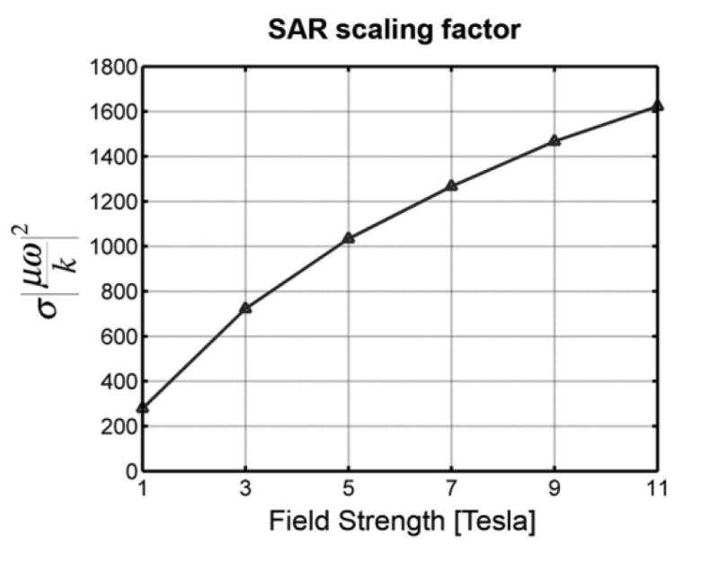
Behavior, as a function of main magnetic field strength, of the scaling factor that pre-multiplies the SAR per unit flip angle for both the case of circular surface coils and the limit case of a full basis set of spherical harmonics. Permeability of free space was used, whereas conductivity and permittivity were set to frequency-dependent in vivo values as in Ref. (26).

When the length of a pulse is shortened, SAR is expected to grow, as transmit currents must be increased to achieve any target level of excitation, and these currents enter quadratically into the expression for SAR. However, in the case of accelerated parallel excitations, ultimate SAR increased only moderately for small acceleration factors, and overall was found to grow more slowly than expected (Figure 7). Relaxation of the constraint on homogeneity of each component coil’s excitation profile in the framework of an accelerated excitation may be in part responsible for this behavior, which nevertheless bears further investigation.

Ultimate intrinsic average global SAR is a global measure of the lowest achievable SAR over the entire pulse duration and the entire volume of the object. Spatial distribution of SAR is, however, very important for in-vivo applications, as “hotspots” may occur in vulnerable anatomic locations (e.g. the orbits for brain imaging studies). Once the current patterns that result in SAR-optimal parallel excitations are calculated, they can be used to compute the associated local RF power deposition at each spatial position and each time period in the excitation. Our results show that, as might be expected, the spatial distribution of SAR within the object depends on its size, since the pattern of interaction of RF fields with dielectric material is dictated by the relation between the incident wavelength and the object dimensions (Figure 8). As acceleration factor increases for parallel excitation, optimum local SAR values near the center of the object become more comparable to the values at its edges (Figure 9), showing that undersampling leads to more RF energy deposition in the middle of the sample. This behavior is less dominant at higher field strengths, suggesting that parallel transmission becomes more effective in resolving aliased positions at higher frequencies. These trends aside, however, peak local SAR is always larger at positions near the surface of the sphere, where the electric field is larger. A quantitative interpretation of peak SAR results for practical safety purposes is delicate and is left to future work.

Both RF shimming and parallel transmission enable complete compensation of B₁ inhomogeneities over a 2D FOV in the ultimate intrinsic case. Even with few coils in fixed combinations, transmit field homogeneity can always be corrected by relying upon a shared gradient- and RF-based excitation pattern to undo the spatial variation of coil sensitivities, although the associated SAR price can be very high (Figure 4). When a transmit array is available, RF shimming can be used to improve homogeneity, while controlling RF power deposition. However, many transmit coils may be needed in order to excite the desired profile. On the other hand, parallel transmission yields good compensation of B₁ inhomogeneities even with small arrays, suggesting once again the potential benefits of this technique at ultra high field strengths. Relative RF shimming performance is improved by choosing appropriately smooth target excitation profiles.

In addition to the shape of the target profile itself, the requirements for profile fidelity have a strong effect on the tradeoff between SAR and homogeneity in multicoil excitation pulse design. The algebraic optimization algorithm employed in this work treats adherence to the target profile as the primary constraint, and minimizes global SAR subject to this constraint. This explains the substantially lower global SAR for RF shimming with an 8-element transmit array (see Figure 4 and 6) as compared with a 12-or 20-element array. In fact, with only 8 coils, close adherence to the target profile is impossible, and remaining degrees of freedom are used for SAR reduction. With more coils, combinations representing a closer match to the target are possible, but these combinations are costly in SAR. Of course, in practice homogeneity need not be prioritized universally over SAR in this manner. A flexible tradeoff between the two pulse design goals is possible using appropriate regularization strategies. The results shown in Figure 6a indicate that the SAR performance of RF shimming approaches may be improved dramatically with regularization. SAR for fully parallel excitations is correspondingly reduced if a similar flexibility in excitation profile is allowed.

SAR results will of course depend as well upon the underlying excitation trajectory, but the general trends demonstrated in this work are expected to be consistent among trajectories. EPI trajectories were used here since they permit a particularly simple formulation of the transmit acceleration process (21), but other excitation trajectories and pulse design approaches are possible (20,38), with some increase in numerical complexity.

One limitation of this study is that in our choice of a uniform target excitation profile (μ = 1) we are constraining both the magnitude and the phase of the optimized B₁ field within the FOV. Although this approach allows us to maintain the linearity of the algorithm and to apply the same SAR optimization to different multi-coil excitation techniques, it is important to remember that, for RF shimming to be effective in certain applications, only the magnitude of B₁ (and of the resulting transverse magnetization) may need to be constrained. Specifying the phase as well in these cases might be unnecessarily restrictive. Indeed, it has been shown that the performance of parallel transmission and multi-spoke pulses can be improved with excitation designs that compensate for B₁ magnitude inhomogeneities, allowing for a small amount of spatial phase variation (39).

Another limitation is the use of a single geometry, but the general theoretical framework outlined in the Theory section applies to any geometry and, for example, it can be extended in a straightforward manner to a cylindrical object by using a different set of basis functions. Furthermore, in this investigation we assumed the spherical sample to be homogeneous, but the general principles should hold for more complex models, incorporating multiple in-vivo tissue types.

It will be important in future work to investigate how sensitive the optimal combination of the individual coils’ excitation patterns may be with respect to calibration errors or small loading perturbations. A better understanding of these questions will help in assessing the practical feasibility of approaching ultimate intrinsic SAR with a relatively small number of transmit elements. In any case, ultimate intrinsic SAR is a theoretical lower bound independent from any specific coil geometry and it can be used as a reference performance target for future designs.

One other practical detail we chose not to include in our circular coil model is the potential effect of inductive or other coupling between transmit coils. This matter has been discussed extensively in the context of early implementations of parallel transmission. However, it is possible that appropriate incorporation of the measured correlation matrix Φ into the SAR optimization will substantially blunt the worst effects of coupling, just as incorporation of the noise correlation matrix in parallel image reconstructions has been shown to blunt the effects of coupling upon SNR (40).

Finally, we chose to assess homogeneity (or adherence to a particular target excitation) in a single 2D FOV. Correcting homogeneity over an entire volume is a more ambitious proposition, and it may even be impossible for RF shimming alone (7). Full volumetric homogeneity correction remains possible with fully parallel transmission, but relatively long pulse durations may be required to add a sufficient number of degrees of freedom to the optimization problem.

CONCLUSIONS

In the present work, fundamental constraints on the lowest possible SAR obtainable with multi-coil excitations were studied with respect to the underlying electrodynamics. In parallel transmission, the capability to transmit tailored excitations with the individual elements of a transmit array enables a high degree of control over B₁ homogeneity in combination with an effective means of SAR management. In RF shimming, relatively low SAR values can be achieved with comparatively simple pulses, but the tradeoff between homogeneity and SAR is less robust. In the case of parallel transmission, ultimate intrinsic SAR varies quite slowly with frequency at the highest field strengths studied, suggesting dramatic potential benefits of this technique for high field imaging and spectroscopy.

APPENDIX A

Minimization of average SAR in RF shimming and parallel transmission

In the Theory section we showed that the problem of finding the set of complex modulation coefficients that minimize ξ while exciting the target profile (see Eq. [31]) reduces to the minimization of the function

$$\xi =\frac{1}{N}\left(\sum _{\rho =1}^N{\mid h_{\rho }\mid }^2\right)\left({\mathbf{\alpha }}^H\mathbf{\Phi }\mathbf{\alpha }\right),$$ [A1]

by varying the quantity α, under the constraint:

$${\mathbf{S}}_{\mathit{FOV}}\mathbf{\alpha }=\frac{{\mathit{\mu }}_{\mathit{FOV}}}{{\mathbf{h}}_{\mathit{FOV}}},$$ [A2]

where α is a [L × 1] vector, S_FOV a [N × L] matrix, Φ a [L × L] matrix and $\frac{{\mathit{\mu }}_{\mathit{FOV}}}{{\mathbf{h}}_{\mathit{FOV}}}$ a [N × 1] vector. The minimization problem can be expressed as a Lagrange function:

$$L=\sum _{l=1}^L\sum _{l^{\prime }=1}^L({\alpha }_{l^{\prime }}^{\ast }{\mathrm{\Phi }}_{l\text{'},l}{\alpha }_l)+\sum _{n=1}^N\sum _{l=1}^L{\lambda }_n(S_{n,l}{\alpha }_l-\frac{{\mu }_n}{h_n})+\sum _{n=1}^N\sum _{l^{\prime }=1}^L({\alpha }_{l^{\prime }}^{\ast }{S}_{n,l^{\prime }}^{\ast }-\frac{{\mu }_n^{\ast }}{h_n^{\ast }}){\lambda }_n^{\ast },$$ [A3]

where λ_n’s are Lagrange multipliers and the scaling factor in Eq. [A1] has been removed for simplicity. Using a matrix formulation, Eq. [A3] becomes:

$$L+\left({\mathbf{\alpha }}^H\mathbf{\Phi }\mathbf{\alpha }\right)+\mathbf{\lambda }\left({\mathbf{S}}_{\mathit{FOV}}\mathbf{\alpha }-\frac{{\mathit{\mu }}_{\mathit{FOV}}}{{\mathbf{h}}_{\mathit{FOV}}}\right)+\left({\mathbf{S}}_{\mathit{FOV}}^H{\mathbf{\alpha }}^H-\frac{{\mathit{\mu }}_{\mathit{FOV}}^H}{{\mathbf{h}}_{\mathit{FOV}}^H}\right){\mathbf{\lambda }}^H.$$ [A4]

If we set to zero the partial derivatives of L with respect to λ, α, α^H and λ^H, we obtain four equations which result in the solution α̃ % of Eq. [33].

In the Theory section we showed that in the case of parallel transmission we can separately optimize the current patterns for each target position, as the RF power ξ in Eq. [19] is positive definite. The minimization problem in Eq [19] can thus be divided in N sub-problems, each of which can be solved with the same method outlined in this section for the case of RF shimming.

APPENDIX B

Calculations of the fields for a coil at an arbitrary position near the surface of the sphere

Eq. [38] provides an expression for the EM field produced by a circular coil whose axis coincides with the z-axis of the laboratory frame (Figure 2). The same expression can be used to calculate the field for an identical circular coil at a different position near the surface of the sphere, by applying an appropriate rotation. The orientation of the reference frame of the rotated coil with respect to the laboratory frame is defined by the angles α and β in Figure 2. So the two reference frames can be superimposed by the consecutive application of two rotations:

$${\mathbf{R}}_{\alpha \beta }={\mathbf{R}}_z(\alpha ){\mathbf{R}}_y(\beta )=\left(\begin{array}{ccc}cos(\alpha )& sin(\alpha )& 0\\ -sin(\alpha )& cos(\alpha )& 0\\ 0& 0& 1\end{array}\right)\left(\begin{array}{ccc}cos(\beta )& 0& -sin(\beta )\\ 0& 1& 0\\ sin(\beta )& 0& cos(\beta )\end{array}\right).$$ [B1]

Pre-multiplying the EM fields of the rotated coil by the rotation matrix R_αβ, we express them with respect to the laboratory frame. Then, in order to evaluate the EM fields at the same positions for both coils, we need to rotate the plane of the FOV backward to its original position, using the inverse of R_αβ.

The transmit RF field produced by the rotated circular coil can thus be calculated as:

$$\begin{array}{l}{\mathit{E}}_{\alpha \beta }^{\text{coil}}(\mathbf{r})={\mathbf{R}}_{\alpha \beta }{\mathit{E}}^{\text{coil}}({\mathbf{R}}_{\alpha \beta }^{-1}\mathbf{r})\\ {\mathit{B}}_{\alpha \beta }^{\text{coil}}(\mathbf{r})={\mathbf{R}}_{\alpha \beta }{\mathit{B}}^{\text{coil}}({\mathbf{R}}_{\alpha \beta }^{-1}\mathbf{r}),\end{array}$$ [B2]

where ℰ^coil and ℬ^coil are the fields of a coil coaxial with the z-axis, defined in Eq. [38]. The resulting values of ${\mathit{B}}_{\alpha \beta }^{\text{coil}}(\mathbf{r})$ were used to generate transmit sensitivities. For computation of the matrix Φ, the quantity $\underset{V}{\int }\sigma (\mathbf{r}){\mathit{E}}_{\alpha \beta }^{\text{coil}}(\mathbf{r})·{\mathit{E}}_{{\alpha }^{\prime }{\beta }^{\prime }}^{\text{coil}\ast }(\mathbf{r})d^3\mathbf{r}$ for appropriately rotated versions of coil electric fields was generated by numerical integration in a common reference frame, since a compact analytic expression is not available.

References

- 1.Van de Moortele PF, Akgun C, Adriany G, Moeller S, Ritter J, Collins CM, Smith MB, Vaughan JT, Ugurbil K. B(1) destructive interferences and spatial phase patterns at 7 T with a head transceiver array coil. Magn Reson Med. 2005;54(6):1503–1518. doi: 10.1002/mrm.20708. [DOI] [PubMed] [Google Scholar]
- 2.Jin J, Chen J. On the SAR and field inhomogeneity of birdcage coils loaded with the human head. Magn Reson Med. 1997;38(6):953–963. doi: 10.1002/mrm.1910380615. [DOI] [PubMed] [Google Scholar]
- 3.Alsop DC, Connick TJ, Mizsei G. A spiral volume coil for improved RF field homogeneity at high static magnetic field strength. Magn Reson Med. 1998;40(1):49–54. doi: 10.1002/mrm.1910400107. [DOI] [PubMed] [Google Scholar]
- 4.Vaughan JT, Adriany G, Snyder CJ, Tian J, Thiel T, Bolinger L, Liu H, DelaBarre L, Ugurbil K. Efficient high-frequency body coil for high-field MRI. Magn Reson Med. 2004;52(4):851–859. doi: 10.1002/mrm.20177. [DOI] [PubMed] [Google Scholar]
- 5.Kangarlu A, Ibrahim TS, Shellock FG. Effects of coil dimensions and field polarization on RF heating inside a head phantom. Magn Reson Imaging. 2005;23(1):53–60. doi: 10.1016/j.mri.2004.11.007. [DOI] [PubMed] [Google Scholar]
- 6.Vaughan JT, Hetherington HP, Otu JO, Pan JW, Pohost GM. High frequency volume coils for clinical NMR imaging and spectroscopy. Magn Reson Med. 1994;32(2):206–218. doi: 10.1002/mrm.1910320209. [DOI] [PubMed] [Google Scholar]
- 7.Hoult DI, Phil D. Sensitivity and power deposition in a high-field imaging experiment. J Magn Reson Imaging. 2000;12(1):46–67. doi: 10.1002/1522-2586(200007)12:1<46::aid-jmri6>3.0.co;2-d. [DOI] [PubMed] [Google Scholar]
- 8.Ibrahim TS, Lee R, Baertlein BA, Abduljalil AM, Zhu H, Robitaille PM. Effect of RF coil excitation on field inhomogeneity at ultra high fields: a field optimized TEM resonator. Magn Reson Imaging. 2001;19(10):1339–1347. doi: 10.1016/s0730-725x(01)00404-0. [DOI] [PubMed] [Google Scholar]
- 9.Vaughan JT. The General Hospital Corporation, assignee. 6, 633, 161. RF coil for imaging system patent. 2003
- 10.Mao W, Smith MB, Collins CM. Exploring the limits of RF shimming for high-field MRI of the human head. Magn Reson Med. 2006;56(4):918–922. doi: 10.1002/mrm.21013. [DOI] [PMC free article] [PubMed] [Google Scholar]
- 11.Van den Berg CA, van den Bergen B, Van de Kamer JB, Raaymakers BW, Kroeze H, Bartels LW, Lagendijk JJ. Simultaneous B1 + homogenization and specific absorption rate hotspot suppression using a magnetic resonance phased array transmit coil. Magn Reson Med. 2007;57(3):577–586. doi: 10.1002/mrm.21149. [DOI] [PubMed] [Google Scholar]
- 12.Hennig J, Weigel M, Scheffler K. Multiecho sequences with variable refocusing flip angles: optimization of signal behavior using smooth transitions between pseudo steady states (TRAPS) Magn Reson Med. 2003;49(3):527–535. doi: 10.1002/mrm.10391. [DOI] [PubMed] [Google Scholar]
- 13.Hargreaves BA, Cunningham CH, Nishimura DG, Conolly SM. Variable-rate selective excitation for rapid MRI sequences. Magn Reson Med. 2004;52(3):590–597. doi: 10.1002/mrm.20168. [DOI] [PubMed] [Google Scholar]
- 14.Hennig J, Scheffler K. Hyperechoes. Magn Reson Med. 2001;46(1):6–12. doi: 10.1002/mrm.1153. [DOI] [PubMed] [Google Scholar]
- 15.Thesen S, Krueger G, Mueller E. Compensation of dielectric resonance effects by means of composite excitation pulses. Proc. 11th Annual Meeting ISMRM; Toronto. 2003. p. 715. [Google Scholar]
- 16.Collins CM, Wang Z, Mao W, Fang J, Liu W, Smith MB. Array-optimized composite pulse for excellent whole-brain homogeneity in high-field MRI. Magn Reson Med. 2007;57(3):470–474. doi: 10.1002/mrm.21172. [DOI] [PMC free article] [PubMed] [Google Scholar]
- 17.Sodickson DK, Manning WJ. Simultaneous acquisition of spatial harmonics (SMASH): fast imaging with radiofrequency coil arrays. Magn Reson Med. 1997;38(4):591–603. doi: 10.1002/mrm.1910380414. [DOI] [PubMed] [Google Scholar]
- 18.Pruessmann KP, Weiger M, Scheidegger MB, Boesiger P. SENSE: sensitivity encoding for fast MRI. Magn Reson Med. 1999;42(5):952–962. [PubMed] [Google Scholar]
- 19.Griswold MA, Jakob PM, Heidemann RM, Nittka M, Jellus V, Wang J, Kiefer B, Haase A. Generalized autocalibrating partially parallel acquisitions (GRAPPA) Magn Reson Med. 2002;47(6):1202–1210. doi: 10.1002/mrm.10171. [DOI] [PubMed] [Google Scholar]
- 20.Katscher U, Bornert P, Leussler C, van den Brink JS. Transmit SENSE. Magn Reson Med. 2003;49(1):144–150. doi: 10.1002/mrm.10353. [DOI] [PubMed] [Google Scholar]
- 21.Zhu Y. Parallel excitation with an array of transmit coils. Magn Reson Med. 2004;51(4):775–784. doi: 10.1002/mrm.20011. [DOI] [PubMed] [Google Scholar]
- 22.Zhu Y. RF power deposition and “g-factor” in parallel transmit. Proc. 14th Annual Meeting ISMRM; Seattle. 2006. p. 599. [Google Scholar]
- 23.Katscher U, Rohrs J, Bornert P. Basic considerations on the impact of the coil array on the performance of Transmit SENSE. Magma. 2005;18(2):81–88. doi: 10.1007/s10334-004-0096-y. Epub 2005 Feb 2011. [DOI] [PubMed] [Google Scholar]
- 24.Ocali O, Atalar E. Ultimate intrinsic signal-to-noise ratio in MRI. Magn Reson Med. 1998;39(3):462–473. doi: 10.1002/mrm.1910390317. [DOI] [PubMed] [Google Scholar]
- 25.Ohliger MA, Grant AK, Sodickson DK. Ultimate intrinsic signal-to-noise ratio for parallel MRI: electromagnetic field considerations. Magn Reson Med. 2003;50(5):1018–1030. doi: 10.1002/mrm.10597. [DOI] [PubMed] [Google Scholar]
- 26.Wiesinger F, Boesiger P, Pruessmann KP. Electrodynamics and ultimate SNR in parallel MR imaging. Magn Reson Med. 2004;52(2):376–390. doi: 10.1002/mrm.20183. [DOI] [PubMed] [Google Scholar]
- 27.Hoult DI. The principle of reciprocity in signal strength calculations - a mathematical guide. Concepts in Magnetic Resonance. 2000;12(4):173–187. [Google Scholar]
- 28.Pauly J, Nishimura DG, Macovski A. A k-space analysis of small-tip-angle excitation. J Magn Reson. 1989;81:43–56. doi: 10.1016/j.jmr.2011.09.023. [DOI] [PubMed] [Google Scholar]
- 29.Saekho S, Yip CY, Noll DC, Boada FE, Stenger VA. Fast-kz three-dimensional tailored radiofrequency pulse for reduced B1 inhomogeneity. Magn Reson Med. 2006;55(4):719–724. doi: 10.1002/mrm.20840. [DOI] [PMC free article] [PubMed] [Google Scholar]
- 30.Setsompop K, Wald LL, Alagappan V, Gagoski B, Hebrank F, Fontius U, Schmitt F, Adalsteinsson E. Parallel RF transmission with eight channels at 3 Tesla. Magn Reson Med. 2006;56(5):1163–1171. doi: 10.1002/mrm.21042. [DOI] [PubMed] [Google Scholar]
- 31.Jackson JD. Classical Electrodynamics. John Wiley & Sons; 1999. [Google Scholar]
- 32.Keltner JR, Carlson JW, Roos MS, Wong ST, Wong TL, Budinger TF. Electromagnetic fields of surface coil in vivo NMR at high frequencies. Magn Reson Med. 1991;22(2):467–480. doi: 10.1002/mrm.1910220254. [DOI] [PubMed] [Google Scholar]
- 33.Wiesinger F, De Zanche N, Pruessmann KP. Approaching ultimate SNR with finite coil arrays. Proc. 13th Annual Meeting ISMRM; Miami Beach. 2005. p. 672. [Google Scholar]
- 34.Wiesinger F. Doctor of Science Thesis. Swiss Federal Institute of Technology; Zurich: 2005. Parallel magnetic resonance imaging: potential and limitations at high fields. [Google Scholar]
- 35.Collins CM, Smith MB. Signal-to-noise ratio and absorbed power as functions of main magnetic field strength, and definition of “90 degrees” RF pulse for the head in the birdcage coil. Magn Reson Med. 2001;45(4):684–691. doi: 10.1002/mrm.1091. [DOI] [PubMed] [Google Scholar]
- 36.Ibrahim TS, Tang L. Insight into RF power requirements and B1 field homogeneity for human MRI via rigorous FDTD approach. J Magn Reson Imaging. 2007;25(6):1235–1247. doi: 10.1002/jmri.20919. [DOI] [PubMed] [Google Scholar]
- 37.Vaughan JT, Garwood M, Collins CM, Liu W, DelaBarre L, Adriany G, Andersen P, Merkle H, Goebel R, Smith MB, Ugurbil K. 7T vs. 4T: RF power, homogeneity, and signal-to-noise comparison in head images. Magn Reson Med. 2001;46(1):24–30. doi: 10.1002/mrm.1156. [DOI] [PubMed] [Google Scholar]
- 38.Zhang Z, Yip CY, Grissom W, Noll DC, Boada FE, Stenger VA. Reduction of transmitter B1 inhomogeneity with transmit SENSE slice-select pulses. Magn Reson Med. 2007;57(5):842–847. doi: 10.1002/mrm.21221. [DOI] [PMC free article] [PubMed] [Google Scholar]
- 39.Setsompop K, Wald LL, Alagappan V, Gagoski BA, Adalsteinsson E. Magnitude least squares optimization for parallel radio frequency excitation design demonstrated at 7 Tesla with eight channels. Magn Reson Med. 2008;59(4):908–915. doi: 10.1002/mrm.21513. [DOI] [PMC free article] [PubMed] [Google Scholar]
- 40.Ohliger MA, Ledden P, McKenzie CA, Sodickson DK. Effects of inductive coupling on parallel MR image reconstructions. Magn Reson Med. 2004;52(3):628–639. doi: 10.1002/mrm.20195. [DOI] [PubMed] [Google Scholar]