RGS9 Concentration Matters in Rod Phototransduction

Abstract

The transduction of light by retinal rods and cones is effected by homologous G-protein cascades whose rates of activation and deactivation determine the sensitivity and temporal resolution of photoreceptor signaling. In mouse rods, the rate-limiting step of deactivation is hydrolysis of GTP by the G-protein-effector complex, catalyzed by the RGS9 complex. Here, we incorporate a “Michaelis module” describing the RGS9 reaction into the conventional scheme for phototransduction and show that this augmented scheme can account precisely for the dominant recovery rate of intact rods in which RGS9 expression varies over a 20-fold range. Furthermore, by screening the parameter space of the scheme with maximum-likelihood methodology, we tested specific hypotheses about the rate constant for rhodopsin deactivation, and about the forward, reverse, and catalytic constants for RGS9-mediated G-protein deactivation. These tests reliably exclude lifetimes >∼50 ms for rhodopsin, and reveal that the dominant time constant of rod photoresponse recovery is 1/(V_max/K_m) for the RGS9 reaction, with k_cat/K_m ≈ 0.04 μm² s⁻¹ and k_cat > 35 s⁻¹ (or K_m > 840 μm⁻²). All together, the new kinetic scheme and analysis explain how and why RGS9 concentration matters in rod phototransduction, and they provide a framework for understanding the molecular mechanisms that rate-limit deactivation in other G-protein systems.

Introduction

Vertebrate rod photoreceptors have long served as a model system for extracting quantitative information about the kinetics of membrane-delimited G-protein coupled receptor (GPCR) signaling (1–5). The outer segment of the rod is densely packed with protein-laden membranous discs on which membrane-delimited G-protein signaling occurs. Photon absorption by the GPCR rhodopsin drives a conformational change to its active state, R^∗ (metarhodopsin II (6), capable of activating the heterotrimeric G-protein, transducin (G_t), by catalyzing GDP-GTP exchange on the α-subunit at a rate of several hundred/s (reviewed in Arshavsky et al. (4)). The GTP-bound, activated form of the transducin α-subunit (G_tα^∗ = G_tα-GTP) binds and relieves the inhibition of the γ-subunit of the membrane-anchored phosphodiesterase (PDE6), creating a catalytically active effector complex (G_tα^∗-E^∗) with a greatly increased rate of hydrolysis of cyclic GMP (7). The resulting decrease in cGMP concentration rapidly leads to closure of cGMP-gated cation channels in the plasma membrane (8,9), producing a decrease in inward current.

Light-induced changes in membrane current can be recorded from intact rods and analyzed to reveal the underlying changes in cGMP concentration, and of G_tα^∗-E^∗ activity as a function of time. One well-established example is the dominant time constant of the recovery of the photoresponse, which reflects the slowest, or rate-limiting step in cascade deactivation (10,11). For light intensities spanning much of the mammalian rod's physiological range (1–3000 photoisomerizations), this step has recently been identified as G_tα^∗-E^∗ deactivation (1), namely GTP hydrolysis catalyzed by the membrane-associated GTPase stimulating complex, comprising RGS9-1 (12), Gβ5-L (13), and R9AP (14). Overexpression of this multimolecular complex (hereafter, simply “RGS9”) dramatically decreases the dominant time constant of photoresponse recovery (1). At first glance, the dependence of the rate-limiting step of recovery on RGS9 concentration may seem surprising, since the GTP hydrolysis that terminates the activity is intrinsic to the G_tα^∗-E^∗ complex. The presumptive explanation is that the rate of formation of the complex of G_tα^∗-E^∗ with RGS9 is much slower than the rate of the subsequent RGS9-catalyzed GTP hydrolysis.

But how much slower? What value of the bimolecular rate constant of RGS9 binding to G_tα^∗-E^∗ is consistent with the observed concentration dependence of shutoff? Is it necessary for the binding to be tight, so that the RGS9- (G_tα^∗-E^∗) complex has a low dissociation rate relative to the catalyzed GTP hydrolysis rate? Does the rate of GTP hydrolysis itself become limiting for recovery when RGS9 expression is sufficiently high, or is the deactivation of R^∗ then rate-limiting? To answer these and related questions, we have developed what we believe is a novel theoretical scheme for the membrane-associated reactions of phototransduction that incorporates a “Michaelis module” for RGS9-catalyzed GTP hydrolysis of the G_tα^∗-E^∗ complex (Fig. 1). Using one set of kinetic parameters, we have described data from rods of transgenic mice in which the concentration of a fundamental regulatory protein (RGS9) varied over a 20-fold range, evaluated the goodness of fit of the model to the data over the entire space of parameters, and tested specific hypotheses about the parameter values. In so doing, we have helped to explain how RGS9 concentration matters in the deactivation of phototransduction.

Figure 1.

(A) Conventional schematic of the disc-associated reactions of the rod phototransduction cascade. (B) Formulation of a “Michaelis module” for the interaction of the RGS9 complex with the activated effector complex, G_tα^∗-E^∗. In the kinetic scheme developed, the Michaelis module (gray box) was substituted for the gray box in A.

Methods

Analysis of saturating flash responses of mouse rods

It has long been recognized that the recovery of the rod photoresponse is dominated by a single first-order deactivation process (10,15), the time constant (τ_D) of which can be easily obtained through analysis of saturating flash responses (10). The saturating flash responses from 88 individual rods of four mouse lines with different RGS9 expression levels investigated by Krispel et al. (1) were reanalyzed to determine the population average T_sat values (Fig. S1 in the Supporting Material). Flash strengths are specified in photoisomerizations/rod (Φ).

Theoretical predictions and statistical analysis

The activation reactions of phototransduction have been analyzed in detail in biophysical terms (3,16). Here, we assume a widely accepted conclusion of the latter investigations (Fig. 1 A), namely, that during its active lifetime (τ_R = 1/k_R), a photoisomerized rhodopsin molecule, R^∗, generates active transducin α-subunits (G_tα^∗) at a steady rate, ν_RG, and that G_tα^∗s in turn stoichiometrically and with negligible delay activate phosphodiesterase (PDE6) catalytic subunits in a complex, G_tα^∗-E^∗, and at a rate, ν_RE, close to ν_RG (17). (Hereafter, since PDE is only active when G_tα^∗ is bound to it, we refer to the complex G_tα^∗-E^∗ simply as E^∗ when there is no loss of clarity.)

With the assumptions just stated, the rate equations governing the kinetic scheme of the Michaelis module of Fig. 1 B were incorporated into the general scheme for the disc-associated reactions and solved analytically with the Laplace transform method (see Section 1.2 in the Supporting Material, and Eq. S1–Eq. S6). The solutions were encoded in a MATLAB (The Mathworks, Natick, MA) script, with the values of the parameters of the model (Table S1) made specifiable via a graphical user interface or by a MATLAB simplex search routine (“fminsearch”). T_sat predictions were compared with the data using several graphical and two numerical metrics, with special emphasis on the maximum-likelihood (ML) method (see Section 1.6 in the Supporting Material). To implement the ML method, a density function (Eq. S17) was formulated that specifies the likelihood, L, that any specific set of parameter values in the five-dimensional “global” space $\Omega =\left\{\overrightarrow{\theta }\right\}=\left\{\left[k_{\mathrm{R}},k_{\mathrm{f}},k_{\text{b}},k_{\text{cat}},E\ast \left(T_{\text{sat}}\right)\right]\right\}$ can account for the empirical T_sat versus log_e(Φ) data: the maximum likelihood estimates (MLEs) are those specific values of the parameters that maximize L. It bears emphasis that there is no a priori guarantee that MLEs are unique (see Section 1.6 in the Supporting Material).

Likelihood ratio tests of hypotheses about the parameters

An important goal of the investigation was to determine what parameter values are incompatible with the results, rather than simply estimating the parameters that produce “best fitting” theoretical curves. The likelihood ratio theorem provides a rigorous method for testing hypotheses about the parameters (see Section 1.6 in the Supporting Material). In essence, this theorem states that in the framework of a parametric model, if a null hypothesis can be formulated as a restriction of the overall parameter space, Ω, to a “subspace” (manifold), ω, of lower dimension, then, when the null hypothesis is true, the log likelihood ratio statistic $-2{\log }_e\left[\hat{L}\left(\omega \right)/\hat{L}(\Omega )\right]$ will be distributed as a χ² distribution with degrees of freedom (df) = dim(Ω) – dim(ω). In this expression, $\hat{L}\left(\omega \right)$ represents the maximum likelihood of the data (a statistic) in the restricted parameter subspace ω, whereas $\hat{L}\left(\mathrm{\Omega }\right)$ is the maximum likelihood in the full parameter space Ω. Here, we consider hypotheses that restrict one of the parameters to specific value, and so dim(Ω) = 5, dim(ω) = 4, and df = 1.

RGS9 expression levels

In addition to the six parameters of the theoretical model, the concentrations of RGS9 in the rods of the four lines of mice also had to be considered to be known with limited precision, as the estimates of the RGS9 levels from quantitative Western analysis showed a nonnegligible variation (see Fig. 3 F of Krispel et al. (1)). In the initial phase of the analysis, we thus held the wild-type RGS9 expression level fixed (in membrane density units) at 100 μm⁻², corresponding roughly to the ratio of 1:269 with rhodopsin (18), and allowed the other three RGS9 levels to be “free but constrained” parameters so that the search analysis was allowed to vary the levels within the empirical 95% confidence intervals for the means of the experimental Western determinations. This approach gave rise to MLEs for the RGS9 expression levels of the four lines of 34, 100, 236, and 360 μm⁻², assuming a membrane density for rhodopsin of 25,000 μm⁻². The RGS9 expression levels were held fixed at these values in all subsequent parameter estimations, goodness of fit calculations, and hypothesis testing. An evaluation of this approach to the variation in the Western data is provided in the Results section.

Results

A Michaelis scheme can account for the RGS9 dependence of rod recovery

Saturating responses of rods from the four RGS9 expression lines were analyzed to determine the average time in saturation (T_sat) produced by each flash strength (Fig. S1). Plotting these T_sat values as a function of the number of photoisomerizations/flash (Φ) on the same semilog plot (Fig. 2 A, symbols) revealed two distinctive features of the data: 1), the slope of the linear relation between T_sat and log_e(Φ) decreases with increasing RGS9 expression; and 2) the magnitude of T_sat likewise declines with increasing RGS9 expression. The critical initial question is, “Can a kinetic scheme incorporating the RGS9 concentration account quantitatively for both of these features of the experimental data?”

Figure 2.

Analysis of time in saturation (T_sat) as a function of flash strength for rods with a 20-fold range of RGS9 expression. (A) Average T_sat data for each of the four lines of mice. The approximate RGS9 expression level, relative to that in WT (1X), is given to the right of the data. The straight lines were generated with the model, with the global maximum likelihood parameter estimates (Table 1, set 1). Error bars are mean ± 1 SE. (B) Deviations of the T_sat data of A from the theoretical predictions: the error bars are identical to those in A, but the vertical scales have been expanded for each level of RGS9 expression to be roughly inversely proportional to the range of the data. Dashed lines identify the zero-deviation level.

To address this question, the rate equations describing the kinetic scheme of Fig. 1 (Eq. S1–Eq. S6) were solved iteratively under the control of a simplex search routine to determine the maximum-likelihood estimates (MLEs) of the parameters (Table 1). The values of T_sat generated by the model with MLE parameters are connected by the straight lines drawn through the experimental data (Fig. 2 A.) The deviations of the theory from the experimental data points are shown for each expression line in Fig. 2 B and reveal no systematic error. Clearly, the model can account well for both the RGS9 dependence of the slopes, and the absolute vertical positions of the data for the different RGS9 expression levels. Moreover, the slopes of the theoretical lines are indistinguishable from the empirical slopes—the dominant recovery time constants (τ_D)—reported by Krispel et al. (1).

Table 1.

Maximum-likelihood estimates of model pand likelihood values

Set	kR (s−1)	kf (μm2 s−1)	kb (s−1)	kcat (s−1)	E∗(Tsat)	kcat/Km(μm2 s−1)	$\log \hat{L}$	χ2	p	Comment/figure
1	33.1	0.051	13.8	52.8	629	0.041	187.0	0.0	NA	Equiv. global MLEs (Fig. 4, inverted triangle)
2	29.0	0.050	15.1	58.5	770	0.040	186.9	0.1	NA	Equiv. global MLEs (Figs. 4 and 5, inverted triangle)
3	20.0	0.045	12.6	130.1	1081	0.041	186.0	1.86	NS	H0: kR = 20 s−1 (Fig. 4, square)
4	12.5	0.043	13.8	154.4	2282	0.040	174.1	25.8	<0.0001	H0: kR = 12.5 s−1 (Fig. 4, triangle)
5	66.2	0.038	0.00	12.5	512	0.038	171.1	31.9	<0.0001	H0: kcat = 12.5 s−1
6	38.8	0.053	7.90	25.0	651	0.040	182.2	9.6	<0.01	H0: kcat = 25 s−1
7	21.5	0.038	0.94	82.2	1200	0.038	185.9	2.3	NS	H0: E∗(Tsat) = 1200
8	20.0	0.038	2.04	105.9	1300	0.038	185.5	3.1	NS	H0: E∗(Tsat) = 1300
9	19.5	0.037	2.13	101.0	1400	0.037	184.8	4.5	<0.05	H0: E∗(Tsat) = 1400

First row, columns 1–5, identifies parameters of the model (see Table 1) and statistics: $-{\log }_e\hat{L}$ is the negative log of the likelihood statistic (Eq. S17) (presented here without the negative sign, for simplicity), whereas ${\chi }^2=-2{\log }_e\left(\hat{\Lambda }\right)$, where $\hat{\Lambda }$ is the likelihood ratio statistic (Eq. S18), predicted to be distributed as a χ² random variable with 1 degree of freedom (df) under the null hypothesis (H₀) in the comment column. The bold entries indicate values at which parameters were held fixed during simplex searches, defining the null hypotheses tested; all other entries in the columns identified by the parameters k_R, k_f, k_b, k_cat, and E^∗(T_sat) are MLEs obtained in simplex searches; k_cat/K_m is a derived, not a primary, parameter. Parameter sets that yielded a value of $-{\log }_e\hat{L}$ within 0.1 of the global minimum, −187 (i.e., within ∼1 part in 2000 of the minimum) were taken to be fully equivalent global MLEs (e.g., sets 1 and 2). In primary screens of grids of several hundred thousand parameter sets (Fig. S5) and in many hundreds of secondary screens with simplex searches, no parameter set was ever found that yielded $-{\log }_e\hat{L}$ < −187.

Assessment of goodness of fit

Although the theoretical predictions generated by the model with MLE parameters provide a good account of the T_sat data, it is nonetheless important to provide a quantitative assessment of the goodness of fit, not just for the global MLE parameters but for other candidates. Such assessment provides a means to ascertain whether the MLE parameters are unique, or whether some other parameter values yield equally good descriptions of the data, and likewise to state which parameter values are reliably excluded. One familiar measure of goodness of fit is the root mean-square error (RMSE). However, because T_sat data obtained from rods expressing different levels of RGS9 have different-magnitude standard deviations, a more appropriate measure is the root mean square of normalized error (RMSNE), i.e., deviations of the data from the theory predictions divided by the within-group standard deviation (Eq. S21). For the theoretical predictions of Fig. 2, RMSNE = 1.0033, whereas the RMSNE of the observations from their empirical mean values is 1.0. Thus, for the model with MLE parameters, the RMS deviation from predictions is only 0.3% greater than it would be for a perfect fit, given the variation inherent in the data.

The second nongraphical measure of goodness of fit employed was the maximum likelihood statistic (Eq. S17), expressed as the negative logarithm, −log_e(L). As can be expected from formal analysis (Fig. S4), −log_e(L) and −log_e[RMSNE] are very closely correlated when the data are well described by the theory. However, −log_e(L) is preferable as a metric of goodness of fit because of the applicability of Wilks's likelihood ratio theorem (see Section S1.6 in the Supporting Material), which provides a means of testing hypotheses about specific parameters of the model, as we now apply to the important issue of the lifetime of R^∗.

Rhodopsin (R^∗) lifetime must be <60 ms

For rods overexpressing RGS9, Krispel et al. (1) found that the dominant recovery time constant approached an apparent minimum of ∼80 ms, and hypothesized that 80 ms might be the lifetime of R^∗ activity. To test this hypothesis, we determined the MLEs of the model with k_R fixed at 1/(0.08 s) = 12.5 s⁻¹. The fit to the data of theoretical curves generated by the model with these parameters is qualitatively poorer (Fig. 3) than that obtained when the simplex search varied k_R to find the best fit (Fig. 2): all the T_sat data for rods underexpressing RGS9 (Fig. 2 A, 0.2X) lie systematically above the theoretical predictions, whereas the data for wild-type (WT) and overexpressors deviate systematically above and below the theory predictions (Fig. 3 B). The qualitative failure of the hypothesis seen in graphical display corresponds well with quantitative analysis: the hypothesis k_R = 12.5 s⁻¹ is strongly rejected (p < 0.0001; Fig. 4). More generally, by performing MLE parameter searches with k_R fixed at various values, we were able to determine which R^∗ lifetimes are consistent with the T_sat data: values of k_R of <19 s⁻¹ are excluded (p < 0.05), so that the R^∗ lifetime τ_R (= 1/k_R) is unlikely to exceed 53 ms (Fig. 4 A).

Figure 3.

Performance of the model with an 80-ms lifetime of R^∗ activity. (A) Predictions of the model with maximum likelihood parameter estimates obtained from simplex searching with k_R fixed at 12.5 s⁻¹. (B) Deviations of the T_sat data from the theoretical predictions; the error bars (mean ± 1 SE) are identical to those in A. Scaling is identical in all aspects to that in Fig. 2, so that the deviations can be directly compared.

Figure 4.

Maximum-likelihood analysis of the lifetime of R^∗. MLEs were obtained with k_R fixed at values specified by the abscissa (the three panels share a common abscissa). (A) Under the null hypothesis that k_R is given by the abscissa value, 2 × the negative log of the likelihood ratio statistic, plotted on the ordinate, will be distributed as a χ² random variable with 1 df (Eq. S18). The dashed lines represent three conventional significance levels: taking p = 0.05 as the cutoff, the analysis rejects k_R < 19 s⁻¹, i.e., τ_R > 53 ms. (B) MLEs of the model parameter E^∗(T_sat) with k_R fixed. (C) MLEs of the model parameter k_f with k_R fixed. The straight lines were fitted by eye. In A–C, inverted triangles represent values obtained in searching with k_R free to vary, i.e., the global MLEs (Table 1, sets 1 and 2). The square represents the values for parameter set 3 of Table 1, which satisfies additional biophysical constraints (Eq. S11–Eq. 15. The smooth curves in each panel are regression lines that help in identifying the values at which the results intersect the statistical rejection criteria, i.e., p levels).

From a purely statistical perspective, however, no value of k_R greater than 20 s⁻¹ can be excluded: many MLE parameter sets found with k_R > 20 s⁻¹ produce statistically equivalent descriptions of the T_sat data. We identify several of these statistically equivalent parameters with distinct symbols in Fig. 4 (Table 1, sets 1–3). Such equivalence is not surprising, because providing that τ_R is adequately shorter than the lifetime of the G_tα^∗-E^∗ complex, the E^∗s will be produced in effect impulsively, so that only their total number, Φ ν_RE τ_R, and not the time course of their production, will affect the late decay of PDE activity. However, to fit the data with values of k_R exceeding 20 s⁻¹, the total number of E^∗s active at the time T_sat, E^∗(T_sat), must decrease systematically (Fig. 4 B). The most plausible, statistically acceptable value of E^∗(T_sat) consistent with the constraints of Eq. S9–Eq. S15 is 1081 (Fig. 4 B, solid square); values <1000 are difficult to reconcile with these constraints (see Biophysical constraints, below). Thus, the overall conclusion is that τ_R for the mouse rod is most likely between 40 and 53 ms.

The MLEs of the other parameters obtained in the simplex searches conducted with k_R fixed are of interest, and in particular the values of k_f, the bimolecular rate constant for formation of the RGS9-G_tα^∗-E^∗ complex (Fig. 4 C). For k_R values fixed at 20–45 s⁻¹, the MLE for k_f increases steadily, but as k_R is increased further, k_f stabilizes at ∼0.064 μm² s⁻¹. The rise in k_f (Fig. 4 C) and decline in E^∗(T_sat) (Fig. 4 B) compensate for shorter R^∗ lifetimes for k_R < 45 s⁻¹; above this latter value, however, compensation for shorter R^∗ lifetime is effected completely by the decline in E^∗(T_sat), as k_f (Fig. 4 C) and all other parameters become constant (results not shown).

k_cat/K_m of the RGS9 reaction determines the dominant recovery rate of the photoresponse

k_f is constrained by k_cat/K_m

To determine the values of k_f consistent with the T_sat data, we used the simplex search process to find MLEs while holding k_f fixed at a series of values (Fig. 5). Values of k_f < ∼0.033 μm² s⁻¹ are strongly rejected (p < 0.01; Fig. 5 A). In contrast, values of k_f > 0.038 μm² s⁻¹ cannot be excluded statistically: the searches revealed a set of Michaelis module parameters that produced statistically equivalent, optimal descriptions of the T_sat data (Fig. 5 A, gray circles). Among this set, k_b seemed wholly unconstrained: holding k_b = 0 or k_b = 100 s⁻¹, for example, yielded equally good fits, providing that values of k_cat and k_f were allowed to compensate. Analysis of these equivalent parameter sets suggested that they obeyed a simple rule, k_cat/K_m ≈ constant, where K_m = (k_b+k_cat)/k_f. Thus, when the χ² statistic of Fig. 5 A is replotted as a function of the values of k_cat/K_m derived from the MLEs of the parameters, the values collapse into a tight cluster in a remarkably narrow range, 0.040 to 0.042 μm² s⁻¹ (Fig. 5 B). This result led us to consider the rule as a general hypothesis, viz., that any set of Michaelis-module parameters that will yield a good description of the T_sat data will satisfy the relation k_cat/K_m ≈ 0.041. This hypothesis explains the inadequacy of values of k_f <0.033 μm² s⁻¹, since k_cat/K_m must always be ≤k_f. We further tested the hypothesis by conducting searches with k_cat/K_m fixed at higher values and found that the hypothesis was supported: k_cat/K_m values >0.047 and <0.036 μm² s⁻¹ were reliably rejected, with a clear minimum at 0.041 (Fig. 5 B). Thus, for k_cat/K_m outside this narrow range, no parameter trade-offs could compensate so as to yield adequate RGS9 concentration dependence.

Figure 5.

Maximum-likelihood analysis of the bimolecular rate of formation, k_f, of the RGS9-G_tα^∗-E^∗ triple complex. (A) Under the null hypothesis that k_f is given by the abscissa value, 2× the negative log of the likelihood ratio statistic, plotted on the ordinate, will be distributed as a χ² random variable with 1 df (Eq. S18); the dashed lines demarcate conventional statistical rejection levels. (B) The χ² values of A have been replotted as a function of the composite rate parameter k_cat/K_m, derived from the values of the MLE parameters k_f, k_b, and k_cat associated with the data points: note that the points plotted as gray circles in A collapse into a tight cluster in B. The squares plot the results of parameter searches in which the ratio k_cat/K_m was forced to adopt the abscissa values 0.045–0.06. The smooth curves are cubic regressions whose purpose is to identify intersections with the rejection significance criteria. The inverted triangle identifies values associated with the global MLE (Table 1, set 2).

How k_cat/K_m governs the dominant recovery rate

The product of k_cat/K_m with the enzyme concentration—in this case, RGS9 density—yields V_max/K_m, the rate constant of depletion of the substrate G_tα^∗-E^∗ when the latter declines below K_m. Formally, if the catalysis of a substrate by an enzyme obeys the quasi-steady-state assumption of Michaelis-Menten kinetics, then the decline of substrate concentration at times t > t₀, such that S(t₀) ≪ K_m is governed by the rate equation

$$\frac{dS}{dt}=-\frac{V_{\text{max}}S}{K_{\mathrm{m}}}$$ (1)

whose solution is an exponential decay:

$$S\left(t\right)=S\left(t_0\right)\exp \left[-\left(V_{\max }/K_m\right)t\right]$$ (2)

Identifying E^∗(t) as the substrate of the RGS9 reactions, these ideas suggested that the exponential decay that underlies the T_sat data of all the RGS9 expressor lines of Fig. 3 might be governed by the rate constant, V_max/K_m, of the RGS9 reaction. However, this suggestion appeared paradoxical, given the apparent complexity of the dependence of the dominant recovery rate on the RGS9 density (r₊; cf. Eq. S7), and, furthermore, the fact that in solving the rate equations we imposed no steady-state condition. The resolution of this paradox is provided by a straightforward (though tedious) MacLaurin expansion of r₊ as a function of RGS9 density, Rgs9. Thus, correct to the second order, Eq. S7 may be approximated by

$$r_{+}=-\frac{k_{\mathrm{cat}}}{K_{\mathrm{m}}}Rgs\mathit{9}+\frac{2k_{\mathrm{cat}}{k}_{\mathrm{b}}}{k_{\mathrm{f}}{K}_{\mathrm{m}}^3}Rgs{\mathit{9}}^2=-\frac{V_{\max }}{K_{\mathrm{m}}}+\frac{2k_{\mathrm{cat}}{k}_{\mathrm{b}}}{k_{\mathrm{b}}+k_{\mathrm{cat}}}{\left[\frac{Rgs\mathit{9}}{K_{\mathrm{m}}}\right]}^2,$$ (3)

where the first term of the second line of Eq. 3 follows from the definition of V_max. The result embodied in Eq. 3 facilitates an understanding of the dependence of the dominant recovery rate constant on the expression level of RGS9, as illustrated in Fig. 6. Here, we plot, as a function of RGS9 expression, k_obs = 1/τ_D, the observed rate-limiting rates of rod response recovery, as measured by Krispel et al. (1), along with three theoretical curves. The thick blue curve plots the full formula for the dominant rate constant, −r₊ (Eq. S7), whereas the dashed and gray curves represent, respectively, the first-order (V_max/K_m) and second-order (Eq. 3) approximations of −r₊ evaluated with the global MLE parameter values (Table 1, set 1). We conclude from this analysis that most of the dependence of k_obs on RGS9 expression level can be explained by a linear dependence on the enzyme density, i.e., k_obs ∼ k_catRgs9/K_m = V_max/K_m, whereas the deviation from V_max/K_m for the highest expression level results from sublinear dependence of the rate −r₊ on Rgs9, as expressed in the opposite-signed, quadratic term of Eq. 3, examined next.

Figure 6.

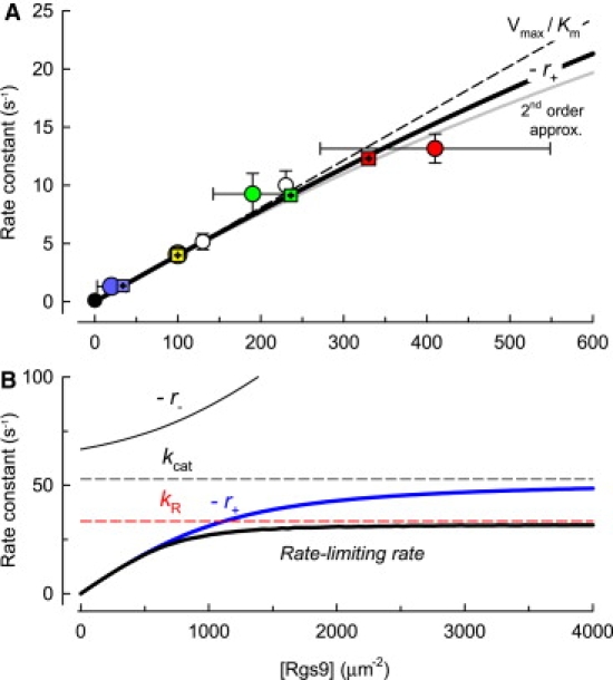
Dependence of the rate-limiting rate of deactivation of phototransduction on RGS9 and predictions of the model. (A) Circles represent empirical rates (k_obs = 1/τ_D) measured by Krispel et al. (1) from rods expressing various levels of RGS9; colored circles are used for the data of the four lines of mice analyzed here, and employ the same color scheme as in Figs. 3 and 4. Horizontal and vertical error bars are 95% confidence intervals. The error terms were derived from an error propagation analysis; the mean value of k_obs for the 4× data is 13.2 s⁻¹, slightly higher than the reciprocal, 12.5 s⁻¹, of the mean value of τ_D. The squares plot the predictions of the model with the global MLE parameters (Table 1, set 1) for the four major expression lines: these points are plotted at the abscissa values estimated initially in the overall parameter estimation process, when the model was applied with the RGS9 levels as free parameters but constrained to lie within the 95% confidence intervals (Methods), and at the ordinate values obtained by analysis of the slope of the “Pepperberg plots” of the E^∗(t) curves generated by the model with MLE parameters (Fig. S2). The smooth curves represent three predicted versions of the rate-limiting recovery rate: 1), the full model (black curve), corresponding over this range of Rgs9 to −r₊ (blue curve); 2), V_max/K_m, the first-order approximation of −r₊ (dashed curve); and 3), the second-order approximation of −r₊ (gray curve). (B) Plot of the rate-limiting rate (black curve) and of −r₊ (blue curve) over a sevenfold greater range of RGS9 densities than in A, along with the rate −r₋ (upper black curve) and two potential rate-limiting cases, the MLE values of k_R (dashed red line) and k_h (dashed black line). k_cat is predicted to become dominant for Rgs9 > 1200 μm⁻²; −r₊ asymptotes to k_cat as expected from enzyme theory, but much more slowly than if the relation were governed by a hyperbolic saturation relation.

Saturation of the dominant recovery rate at high levels of RGS9

Krispel et al. (1) found an apparent 80-ms minimum for τ_D for rods with high RGS9 expression; this minimum corresponds in Fig. 6 A to the highest observed rate, k_obs = 12.5 s⁻¹ (red circle). As an alternative to the hypothesis that k_obs = k_R under such conditions, they proposed “that GTP hydrolysis is sped maximally,” viz., that the saturated rate of GTP hydrolysis (k_cat) dominates the recovery kinetics. We tested this hypothesis by searching for MLEs subject to the restriction k_cat = 12.5 s⁻¹: the hypothesis is rejected with p < 0.0001 (Table 1, set 5). Likewise, the hypothesis k_cat = 25 s⁻¹ is strongly rejected (p < 0.01, Table 1, set 6). Further, such analysis leads to the conclusion that for the model to describe the T_sat data, not only must the parameters of the Michaelis module satisfy k_cat/K_m ≈ 0.04, but also k_cat must be at least 35 s⁻¹. This value is similar to that measured in vitro (30–50 s⁻¹ (19,20). It is notable that a k_cat value of at least 35 s⁻¹ is equivalent to having K_m at least 850 μm⁻², given the restriction that k_cat/K_m ≈ 0.04 μm² s⁻¹. We thus conclude that the Krispel et al.'s (1) characterization of the highest observed recovery rate as “saturating” is incorrect. Rather, we think that their results are better accounted for by the deceleration of the dominant rate due to its sublinear dependence on Rgs9 (Eq. 3), combined with allowance for potential error in the Western blot analysis of RGS9 levels (Fig. 6 A, horizontal error bars).

At what RGS9 level would the GTP hydrolysis rate constant k_cat become rate-limiting for photoresponse recovery? To address this question, in Fig. 6 B, we plot the three MLE rate constants that govern E^∗(t), i.e., k_R, −r₊, and −r₋ (Eq. S7 and Eq. S8), over a wider range of RGS9 levels than used in Fig. 6 A, along with the MLE value of k_cat for comparison. At each RGS9 level specified by the abscissa, the theoretically predicted dominant recovery rate is the rate constant of the three that has the smallest value. From this graphical analysis, it can be seen that k_R would become rate-limiting for recovery when RGS9 density exceeds 1100 μm⁻². At RGS9 levels >3000 μm⁻², the composite Michaelis module rate constant −r₊ does indeed saturate at k_cat, but k_cat would not rate-limit recovery unless k_R exceeded k_cat.

Why the model fails with an 80-ms lifetime of R^∗

Why does the model with an R^∗ lifetime >∼50 ms fail to account for the T_sat data? Insight into this problem can be obtained from inspection of Fig. 7, where the dependence of k_obs on Rgs9 is shown, as in Fig. 6, but with theoretical rates generated by the model with MLE parameters obtained when k_R was constrained to be 12.5 s⁻¹ (as in Fig. 4). Subject to this constraint, the simplex searching found values of the Michaelis module parameters that give a value of k_cat/K_m = 0.040 μm² s⁻¹, equivalent to that yielded by the global MLEs (Table 1, rows 1, 2, and 4). However, it is predicted that k_R will become dominant only as Rgs9 increases to >400 μm⁻², and in the transitional range of Rgs9 between dominance by V_max/K_m and dominance by k_R, the predicted rate-limiting recovery rates are reliably lower than k_obs. Thus, the failure of the model with an R^∗ lifetime of 80 ms arises from its inability to simultaneously satisfy the essentially linear RGS9 dependence of k_obs on Rgs9 for expression levels up to twofold above WT and rate saturation at k_R: the predicted transition between linear dependence on Rgs9 and saturation at k_R is too gradual to account for the data.

Figure 7.

Theoretical basis for the failure of the model with τ_R = 80 ms to explain the observed dependence of the rate-limiting rate on RGS9 expression level. (A) The results in Fig. 6 have been replotted with theoretical curves generated by the model with the MLEs obtained in simplex searching with k_R = 12.5 s⁻¹ (Table 1, set 4). (B) The theory traces in A are plotted over an ∼3-fold greater range of RGS9 densities, along with dashed lines representing k_R and k_cat.

Biophysical constraints on the value of E^∗(T_sat)

In describing the T_sat data, the lifetime of R^∗ used in the model can be almost arbitrarily short (k_R arbitrarily large), provided E^∗(T_sat) is sufficiently small to compensate (Fig. 4). A similar compensatory tradeoff arose between k_f and E^∗(T_sat) (Fig. 5). These ambiguities could be removed or lessened if a lower limit for E^∗(T_sat) could be deduced from considerations other than the statistical analysis of the T_sat data. We explored this possibility by evaluating the defining relation for E^∗(T_sat) (Eq. S11), as constrained by Eq. S12–Eq. S15, with published or derivable estimates of the parameters involved.

No plausible values for the parameters of Eq. S11–Eq. S15 that predicted E^∗(T_sat) to be much less than ∼1200 could be found. Table S2 provides a set of values of the parameters that are mutually consistent and that yield E^∗(T_sat) = 1181. Several of these values were obtained from the large rod outer segments of amphibia at room temperature; we have thus made educated guesses based on the literature to accommodate the temperature, volume, or other known species differences, as indicated. To determine whether the discrepancy between E^∗(T_sat) = 1200 and the global MLE values, E^∗(T_sat) = 629–770 (Table 1, sets 1 and 2), is material, we performed simplex searches with the model subject to the restrictions E^∗(T_sat) = 1200, 1300, and 1400: although the first two values cannot be rejected, the value 1400 was rejected (p < 0.05; Table 1, sets 7–9), and larger values of E^∗(T_sat) were rejected at still more stringent significance levels. In summary, the application of the model to the T_sat data restricts E^∗(T_sat) to be <1300, whereas the independent biophysical constraints embodied in Eq. S11–Eq. S15 require it to be >∼1200.

Although the range of acceptable values of E^∗(T_sat) appears tightly constrained, it must be reiterated that, for any specific set of parameter values and flash intensity, E^∗(T_sat) varies in direct proportion to ν_RE, the rate of production of active PDE units per R^∗ (Supporting Material). In all the simplex searches, ν_RE for mouse rods was set to 375 s⁻¹, based on a reasonable extrapolation from in vitro amphibian data (17). However, if a higher value for ν_RE had been adopted, the estimates of E^∗(T_sat) with the model would have increased proportionately. The difficulty in finding parameters for Eq. S11–Eq. S15 that are consistent with E^∗(T_sat) values <1200 suggests that in intact mammalian rods, ν_RE may indeed be >375 s⁻¹. Heck and Hofmann (21), in a thoroughgoing analysis of a light-scattering signal attributable to G_t activation, conclude that in the living mammalian rod the rate of activation of G_t per R^∗ would be 700 s⁻¹. Adopting this latter rate and assuming a high coupling efficiency between G_tα∗ and PDE, so that ν_RE is close to 700 s⁻¹, would resolve many of the difficulties in finding a set of parameters consistent with Eq. S11.

Discussion

The dominant photoresponse recovery rate corresponds to V_max/K_m of the RGS9 reaction

Our analysis has revealed the mechanistic basis of the exponential decay that gives rise to the dominant recovery time constant, τ_D, of the rod flash response. Once R^∗ activity has decayed and is no longer producing G_tα-GTP, the substrate G_tα∗-E^∗ (G_tα-GTP-E^∗) for the RGS9 reaction decays with “tail phase” enzyme kinetics, i.e., with the rate constant k_obs = 1/τ_D ≈ (k_catRgs9)/K_m = V_max/K_m (Eqs. 1–3 and Fig. 6 A).

The analysis also reveals that the value of τ_D (80 ms) for rods of the line with the highest level of RGS9 expression (1) is not set by the RGS9 turnover number, k_cat (Fig. 2): the hypothesis k_cat = 12.5 s⁻¹ is very strongly rejected (Table 1). However, the analysis supports the conclusions that the value of τ_D of 80 ms is determined by the RGS9 reaction (Fig. 6 A), and that still higher levels of RGS9 expression could yield still faster photoresponse kinetics (Fig. 6 B), providing the lifetime of R^∗ is appropriately brief. This latter conclusion has important implications for the temporal regulation of other G-protein signaling systems. In particular, RGS9 is known to be essential for normal deactivation of cone photoreceptor signaling (22), and cones express up to 10-fold higher levels of RGS9 than rods (23,24). If k_cat of the RGS9 reaction in cones exceeds 50 s⁻¹ as our analysis reveals it does in rods (Table 1), and if the K_m is comparable in the two types of photoreceptors, the higher expression in cones should give rise to a faster deactivation of G_tα-GTP-E^∗ and a smaller dominant recovery time constant. Nonetheless, whether the faster deactivation of cones is rate-limited by k_cat or k_R (cf. Fig. 6 B) remains an open question.

The lifetime of R^∗ in the mouse rod at 37°C is <60 ms

Our results strongly reject the hypothesis that the lifetime τ_R of R^∗ activity is >53 ms (Figs. 3 and 4). This conclusion is explicitly valid only for the intensities of the T_sat data (Fig. 2), which range from ∼200 to 2000 photoisomerizations/rod. Above this intensity range the dominant recovery time constant of mouse rods slows (25,1), likely due to the formation of G_tα^∗ in excess of PDEγ (18). For lower light intensities, including those that produce single isomerizations, it is reasonable to infer that the R^∗ lifetime is also <60 ms, since predictions of E^∗(t) with the model are linearly dependent on flash strength, and this linearity underlies the T_sat predictions (Fig. 2). The biophysical basis of the linearity is that the reactions involved take place in or at the rod disc membrane, and the intensities involved produce no more than ∼1 isomerization/disc face. Presumably common kinetic processes on each disc face produce on average identical pulses of PDE activity, E^∗(t), in response to a single photoisomerization on that disc face.

An exception to strict linearity of E^∗(t) for this range of flash strengths might occur if the decline in calcium that accompanies the light response could alter the lifetime of R^∗ dynamically, that is, shorten the lifetime during the light response. Such dynamic feedback could shorten the R^∗ lifetime in response to strong flashes, which cause larger and more rapid changes in intracellular free calcium, relative to the lifetime governing the response to dim flashes, which cause smaller changes in calcium. However, evidence from WT and RGS9-overexpressing rods argues that any such dynamic effect on the R^∗ lifetime is negligible. In the rods whose responses are considered here, the tail phase of the single photon response decays exponentially, and there is remarkable agreement between the tail-phase time constant (τ_rec) for dim-flash responses and the dominant recovery time constant (τ_D) extracted from the analysis of saturating flashes (1). Since τ_rec and τ_D are 80 ms for the “4X” overexpressor, it follows that under the conditions of the single-photon response, τ_R is no greater than 80 ms, and thus it seems unlikely that R^∗ lifetime is substantially longer for dim flashes than for saturating ones.

The normal deactivation of R^∗ at all flash strengths is biochemically complex, requiring both phosphorylation of C-terminal residues by GRK1 (26,27) and subsequent arrestin binding (28). Although a biochemically explicit and testable representation of rapid R^∗ deactivation may emerge, its approximation in this investigation as an exponential decay is inconsequential for analysis of the kinetics of RGS9-catalyzed GTP hydrolysis. Specifically, the finding that all values of τ_R < ∼50 ms are consistent with the T_sat data (Fig. 4 A) reveals that it is the brevity of the R^∗ lifetime relative to that of the G_tα^∗-E^∗ complex, not the kinetic form, that is critical to the conclusions.

A consequence of the ∼7-fold ratio of τ_E to τ_R (Table 1, sets 1 and 2) in WT rods is that the E^∗s produced during the brief lifetime of R^∗ can be integrated in the response: nearly all the E^∗s produced are for a time simultaneously active, so that their signal is maximally efficient. A similar efficiency apparently applies to the rods of cold-blooded vertebrates whose phototransduction is ∼10-fold slower. The dominant recovery time constant, τ_D, of amphibian rods has consistently been determined to be 2–2.5 s, and a second, “nondominant” constant of ∼0.5 s for the disc-associated reactions has also been uncovered (10,11,29,30). Interpreting τ_D as RGS9-catalyzed G_tα^∗-E^∗ decay (τ_E), and the nondominant time constant as R^∗ deactivation (τ_R) yields a signaling efficiency similar to that of mammalian rods. The high ratio of τ_E to τ_R in vertebrate rods ensures that nearly all E^∗s produced during the lifetime of R^∗ are simultaneously active for at least a brief period, whereas if the E^∗ lifetime were shorter or the R^∗ lifetime longer, there would be a net loss of signal.

References

- 1.Krispel C.M., Chen D., Melling N., Chen Y.J., Martemyanov K.A. RGS expression rate-limits recovery of rod photoresponses. Neuron. 2006;51:409–416. doi: 10.1016/j.neuron.2006.07.010. [DOI] [PubMed] [Google Scholar]
- 2.Stryer L. Cyclic GMP cascade of vision. Annu. Rev. Neurosci. 1986;9:87–119. doi: 10.1146/annurev.ne.09.030186.000511. [DOI] [PubMed] [Google Scholar]
- 3.Pugh E.N., Jr., Lamb T.D. Amplification and kinetics of the activation steps in phototransduction. Biochim. Biophys. Acta. 1993;1141:111–149. doi: 10.1016/0005-2728(93)90038-h. [DOI] [PubMed] [Google Scholar]
- 4.Arshavsky V.Y., Lamb T.D., Pugh E.N., Jr. G proteins and phototransduction. Annu. Rev. Physiol. 2002;64:153–187. doi: 10.1146/annurev.physiol.64.082701.102229. [DOI] [PubMed] [Google Scholar]
- 5.Luo D.G., Xue T., Yau K.W. How vision begins: an odyssey. Proc. Natl. Acad. Sci. USA. 2008;105:9855–9862. doi: 10.1073/pnas.0708405105. [DOI] [PMC free article] [PubMed] [Google Scholar]
- 6.Hofmann K.P. Photoproducts of rhodopsin in the disk membrane. Photobiochem. Photobiophys. 1986;13:309–327. [Google Scholar]
- 7.Wensel T.G., Stryer L. Reciprocal control of retinal rod cyclic GMP phosphodiesterase by its γ subunit and transducin. Proteins. 1986;1:90–99. doi: 10.1002/prot.340010114. [DOI] [PubMed] [Google Scholar]
- 8.Cobbs W.H., Pugh E.N., Jr. Kinetics and components of the flash photocurrent of isolated retinal rods of the larval salamander, Ambystoma tigrinum. J. Physiol. 1987;394:529–572. doi: 10.1113/jphysiol.1987.sp016884. [DOI] [PMC free article] [PubMed] [Google Scholar]
- 9.Karpen J.W., Zimmerman A.L., Stryer L., Baylor D.A. Gating kinetics of the cyclic-GMP-activated channel of retinal rods: flash photolysis and voltage-jump studies. Proc. Natl. Acad. Sci. USA. 1988;85:1287–1291. doi: 10.1073/pnas.85.4.1287. [DOI] [PMC free article] [PubMed] [Google Scholar]
- 10.Pepperberg D.R., Cornwall M.C., Kahlert M., Hofmann K.P., Jin J. Light-dependent delay in the falling phase of the retinal rod photoresponse. Vis. Neurosci. 1992;8:9–18. doi: 10.1017/s0952523800006441. [DOI] [PubMed] [Google Scholar]
- 11.Lyubarsky A., Nikonov S., Pugh E.N., Jr. The kinetics of inactivation of the rod phototransduction cascade with constant Ca2+i. J. Gen. Physiol. 1996;107:19–34. doi: 10.1085/jgp.107.1.19. [DOI] [PMC free article] [PubMed] [Google Scholar]
- 12.He W., Cowan C.W., Wensel T.G. RGS9, a GTPase accelerator for phototransduction. Neuron. 1998;20:95–102. doi: 10.1016/s0896-6273(00)80437-7. [DOI] [PubMed] [Google Scholar]
- 13.Makino E.R., Handy J.W., Li T., Arshavsky V.Y. The GTPase activating factor for transducin in rod photoreceptors is the complex between RGS9 and type 5 G protein β subunit. Proc. Natl. Acad. Sci. USA. 1999;96:1947–1952. doi: 10.1073/pnas.96.5.1947. [DOI] [PMC free article] [PubMed] [Google Scholar]
- 14.Hu G., Wensel T.G. R9AP, a membrane anchor for the photoreceptor GTPase accelerating protein, RGS9–1. Proc. Natl. Acad. Sci. USA. 2002;99:9755–9760. doi: 10.1073/pnas.152094799. [DOI] [PMC free article] [PubMed] [Google Scholar]
- 15.Hodgkin A.L., Nunn B.J. Control of light-sensitive current in salamander rods. J. Physiol. 1988;403:439–471. doi: 10.1113/jphysiol.1988.sp017258. [DOI] [PMC free article] [PubMed] [Google Scholar]
- 16.Lamb T.D., Pugh E.N., Jr. A quantitative account of the activation steps involved in phototransduction in amphibian photoreceptors. J. Physiol. 1992;449:719–758. doi: 10.1113/jphysiol.1992.sp019111. [DOI] [PMC free article] [PubMed] [Google Scholar]
- 17.Leskov I.B., Klenchin V.A., Handy J.W., Whitlock G.G., Govardovskii V.I. The gain of rod phototransduction: reconciliation of biochemical and electrophysiological measurements. Neuron. 2000;27:525–537. doi: 10.1016/s0896-6273(00)00063-5. [DOI] [PubMed] [Google Scholar]
- 18.Martemyanov K.A., Krispel C.M., Lishko P.V., Burns M.E., Arshavsky V.Y. Functional comparison of RGS9 splice isoforms in a living cell. Proc. Natl. Acad. Sci. USA. 2008;105:20988–20993. doi: 10.1073/pnas.0808941106. [DOI] [PMC free article] [PubMed] [Google Scholar]
- 19.Lishko P.V., Martemyanov K.A., Hopp J.A., Arshavsky V.Y. Specific binding of RGS9-Gβ 5L to protein anchor in photoreceptor membranes greatly enhances its catalytic activity. J. Biol. Chem. 2002;277:24376–24381. doi: 10.1074/jbc.M203237200. [DOI] [PubMed] [Google Scholar]
- 20.Baker S.A., Martemyanov K.A., Shavkunov A.S., Arshavsky V.Y. Kinetic mechanism of RGS9–1 potentiation by R9AP. Biochemistry. 2006;45:10690–10697. doi: 10.1021/bi060376a. [DOI] [PubMed] [Google Scholar]
- 21.Heck M., Hofmann K.P. Maximal rate and nucleotide dependence of rhodopsin-catalyzed transducin activation: initial rate analysis based on a double displacement mechanism. J. Biol. Chem. 2001;276:10000–10009. doi: 10.1074/jbc.M009475200. [DOI] [PubMed] [Google Scholar]
- 22.Lyubarsky A.L., Naarendorp F., Zhang X., Wensel T., Simon M.I. RGS9–1 is required for normal inactivation of mouse cone phototransduction. Mol. Vis. 2001;7:71–78. [PubMed] [Google Scholar]
- 23.Cowan C.W., Fariss R.N., Sokal I., Palczewski K., Wensel T.G. High expression levels in cones of RGS9, the predominant GTPase accelerating protein of rods. Proc. Natl. Acad. Sci. USA. 1998;95:5351–5356. doi: 10.1073/pnas.95.9.5351. [DOI] [PMC free article] [PubMed] [Google Scholar]
- 24.Zhang X., Wensel T.G., Kraft T.W. GTPase regulators and photoresponses in cones of the eastern chipmunk. J. Neurosci. 2003;23:1287–1297. doi: 10.1523/JNEUROSCI.23-04-01287.2003. [DOI] [PMC free article] [PubMed] [Google Scholar]
- 25.Lyubarsky A.L., Pugh E.N., Jr. Recovery phase of the murine rod photoresponse reconstructed from electroretinographic recordings. J. Neurosci. 1996;16:563–571. doi: 10.1523/JNEUROSCI.16-02-00563.1996. [DOI] [PMC free article] [PubMed] [Google Scholar]
- 26.Chen J., Makino C.L., Peachey N.S., Baylor D.A., Simon M.I. Mechanisms of rhodopsin inactivation in vivo as revealed by a COOH- terminal truncation mutant. Science. 1995;267:374–377. doi: 10.1126/science.7824934. [DOI] [PubMed] [Google Scholar]
- 27.Chen C.K., Burns M.E., Spencer M., Niemi G.A., Chen J. Abnormal photoresponses and light-induced apoptosis in rods lacking rhodopsin kinase. Proc. Natl. Acad. Sci. USA. 1999;96:3718–3722. doi: 10.1073/pnas.96.7.3718. [DOI] [PMC free article] [PubMed] [Google Scholar]
- 28.Xu J., Dodd R.L., Makino C.L., Simon M.I., Baylor D.A. Prolonged photoresponses in transgenic mouse rods lacking arrestin. Nature. 1997;389:505–509. doi: 10.1038/39068. [DOI] [PubMed] [Google Scholar]
- 29.Matthews H.R. Actions of Ca2+ on an early stage in phototransduction revealed by the dynamic fall in Ca2+ concentration during the bright flash response. J. Gen. Physiol. 1997;109:141–146. doi: 10.1085/jgp.109.2.141. [DOI] [PMC free article] [PubMed] [Google Scholar]
- 30.Nikonov S., Engheta N., Pugh E.N., Jr. Kinetics of recovery of the dark-adapted salamander rod photoresponse. J. Gen. Physiol. 1998;111:7–37. doi: 10.1085/jgp.111.1.7. [DOI] [PMC free article] [PubMed] [Google Scholar]
Associated Data
This section collects any data citations, data availability statements, or supplementary materials included in this article.