Effects of Charge on Osmotic Reflection Coefficients of Macromolecules in Fibrous Membranes

Abstract

A model based on continuum hydrodynamics and electrostatics was developed to predict the combined effects of molecular charge and size on the osmotic reflection coefficient (σ_o) of a macromolecule in a fibrous membrane, such as a biological hydrogel. The macromolecule was represented as a sphere with a constant surface charge density, and the membrane was assumed to consist of an array of parallel fibers of like charge, also with a constant surface charge density. The flow was assumed to be parallel to the fiber axes. The effects of charge were included by computing the electrostatic free energy for a sphere interacting with an array of fibers. It was shown that this energy could be approximated using a pairwise additivity assumption. Results for σ_o were obtained for two types of negatively charged fibers, one with properties like those of glycosaminoglycan chains, and the other for thicker fibers having a range of charge densities. Using physiologically reasonable fiber spacings and charge densities, σ_o for bovine serum albumin in either type of fiber array was shown to be much larger than that for an uncharged system. Given the close correspondence between σ_o and the reflection coefficient for filtration, the results suggest that the negative charge of structures such as the endothelial surface glycocalyx is important in minimizing albumin loss from the circulation.

Introduction

Polymeric hydrogels containing networks of proteins, glycosaminoglycans (GAG), and other biopolymers, and consisting mostly of water, are present throughout the body. They can be viewed as arrays of fibers with fluid-filled interstices. The fibers may be single polymeric chains or multichain aggregates, and their arrangement may be highly ordered or relatively random. Examples of such fibrous materials include the glycocalyx coatings of cells, junctional complexes in endothelia and epithelia, basement membranes, and interstitial matrices. The resistances of fibrous materials to the transport of water and solutes impact numerous physiological functions, often controlling microvascular and other permeability properties and generally affecting the extracellular movement of nutrients, cytokines, and therapeutic drugs. Often, the fibers have a net electrical charge. We are concerned here with osmotic flow through such materials and, less directly, the convective transport of macromolecules. In particular, we are interested in the effects of molecular charge, as well as molecular size, on osmosis and convection through membranes consisting of fibrous hydrogels. Our focus is on macromolecular solutes (such as globular proteins), which are large enough and rigid enough to be viewed as hydrodynamic particles.

The ability of a solute to induce an osmotic flow is measured by its osmotic reflection coefficient (σ_o). When a single solute is present, the transmembrane volume flux (or superficial fluid velocity, v) is related to the mechanical (ΔP) and osmotic (ΔΠ) pressure differences as

$$v=K\left(\Delta P-{\sigma }_{\text{o}}\Delta \Pi \right),$$ (1)

where K is the hydraulic permeability. In a membrane with pores or interfiber spaces small enough to completely exclude the solute, σ_o = 1 and the full osmotic potential of the solute is realized; if the spaces are so large that the membrane does not discriminate between solute and water molecules, σ_o = 0 and osmosis is absent. In general, there is intermediate behavior, such that 0 ≤ σ_o ≤ 1. For solutions with multiple solutes, Eq. 1 can be generalized by replacing σ_oΔΠ by a sum of such terms.

The ability of a membrane to sieve a solute in a filtration process is measured by the reflection coefficient for filtration (σ_f). If transmembrane convection is dominant and diffusion is negligible (which requires that Pe, the Peclet number based on membrane thickness, be large), the solute flux (N) is given by

$$N=C_{0}v\left(1-{\sigma }_{\text{f}}\right)\left(\text{Pe}>>1\right),$$ (2)

where C₀ is the concentration at the upstream membrane surface (1). As with the osmotic reflection coefficient, σ_f = 1 if the solute is completely excluded and σ_f = 0 if the membrane is unselective. The correspondence between σ_o and σ_f exists also for intermediate situations. That is, hydrodynamic models for osmosis and filtration in porous membranes have shown that σ_o ≅ σ_f for all combinations of solute and pore size, and solute and pore charge (2–5). Although such theories for fibrous membranes are less well developed, it is reasonable to assume that the two reflection coefficients again will be equal, or nearly so. For flow parallel to an array of regularly spaced fibers, and in the absence of charge effects, the equality has been shown to be exact, provided that the tendency of a confined, freely suspended sphere to lag somewhat behind the local fluid velocity is ignored (6). Thus, although the theory developed here is for σ_o, the results provide insight also into the effects of molecular charge on σ_f. Because the hydrodynamic problems that must be solved to predict σ_f tend to be much more difficult than those needed to estimate σ_o (7), computing σ_o is a logical first step in examining hindered convection in complex geometries such as fiber arrays.

The objective of this work was to evaluate σ_o for charged spheres in membranes consisting of regular arrays of fibers of like charge. As in the analysis of Zhang et al. (6) for neutral spheres and fibers, the flow was assumed to be parallel to the fiber axes. An important subproblem was how to estimate the change in electrostatic energy associated with placing a charged sphere inside a periodic array of charged fibers. This energy was evaluated using continuum double-layer calculations for a sphere interacting with a single charged cylinder, together with a pairwise additivity approximation. Pairwise additivity of energies was tested using exact results generated for a sphere interacting with two cylinders, and found to work reasonably well. The electrostatic energies were combined with a viscous flow model to compute σ_o as a function of the fiber volume fraction, fiber and sphere charge densities, and fiber and sphere size.

Theory

Model geometry

Long fibers, aligned with the z axis, were assumed to be arranged on a hexagonal lattice. Fig. 1 shows a central fiber surrounded by an inner ring of six nearest neighbors and a second ring of twelve next-nearest neighbors. Certain symmetry planes are indicated by dashed lines. The hexagonal pattern was assumed to repeat indefinitely. Also shown (solid circle) is a spherical macromolecule positioned within the inner ring. The flow was assumed to be normal to the plane of the figure (in the z direction).

Figure 1.

Parallel fibers arranged on a hexagonal lattice. The fibers are shaded and certain symmetry planes are indicated by the dashed lines. A spherical macromolecule (solid) is shown near the central fiber.

Fig. 2 is an enlargement of the region near the central fiber, with the key geometric parameters shown. The sphere radius is a, the fiber radius is b, and the surface-to-surface fiber separation is H. Cylindrical radial and angular coordinates, based on the central fiber, are r and θ. Because of the symmetry, it was sufficient to consider only 0 ≤ θ ≤ π/6. Following Happel (8) and Zhang et al. (6), in the flow calculations the geometry was simplified to an annulus by replacing the hexagonal boundary by a circle of radius R. This flow radius was chosen to maintain the same open area per fiber. The relationship among R, b, and H is

$$R=\frac{3^{1/4}}{\sqrt{2\pi }}\left(2b+H\right)\text{.}$$ (3)

Figure 2.

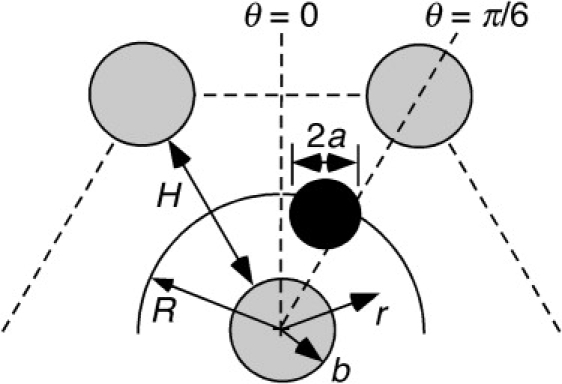
Enlargement of the hexagonal fiber lattice, showing a central fiber and two nearest neighbors (shaded), a spherical macromolecule (solid), local cylindrical coordinates, and key lengths. The surface r = R is the outer boundary of the annular region used in the osmotic flow calculations, with R chosen to yield the same open area per fiber as in the hexagonal array.

The largest sphere that will fit anywhere within such an array has a radius

$$a_{\text{m}}=\frac{2b+H}{\sqrt{3}}-b\text{.}$$ (4)

Thus, σ_o = 1 for a ≥ a_m. A sphere with H + b – R < a < a_m will fit at some positions, but will have its center limited to angular positions such that 0 ≤ θ ≤ θ_m, where

$${\theta }_{\text{m}}=\frac{\pi }{6}-{\cos }^{-1}\left[\frac{r^2+{\left(2b+H\right)}^2-{\left(a+b\right)}^2}{2r\left(2b+H\right)}\right]\text{.}$$ (5)

This maximum angle is affected, of course, by the radial position of the sphere center (r). Smaller spheres (a < H + b – R) are restricted sterically only by the central fiber. To fit, it is necessary only that their centers be positioned at r > a + b.

Physical assumptions

The membrane thickness (L, also the fiber length) was assumed to greatly exceed R, which has two consequences. First, the resistances to water and solute transport across the interfaces at z = 0 and z = L will be negligible relative to those within the fiber matrix, allowing thermodynamic equilibrium to be assumed between the internal and external solutions at those boundaries. This is the usual assumption made in analyzing membrane transport processes. Second, the lubrication approximation can be applied to the equations of motion, as in the analogous problem involving long, cylindrical pores (9). This greatly simplifies the hydrodynamic problem.

The mobile macromolecules were modeled as spheres with a specified surface charge density; the surface charge density of the fibers was also constant. The electrolyte was assumed to consist of univalent anions and cations, each of negligible size relative to the macromolecule or fibers. The macromolecule solutions were assumed to be dilute enough to make solute-solute interactions negligible. The bulk electrolyte concentrations on the two sides of the membrane were taken to be equal, so that osmosis results only from an imbalance in macromolecule concentrations. No restrictions were placed on the Debye length or surface charge densities, but to avoid situations where electrostatic interactions might cause macromolecule adsorption, results were obtained only for particles and fibers of like charge.

Following the approach in Anderson and Malone (9) and subsequent models of osmotic flow through membranes that permit solute entry (3–6), the macromolecule was assumed to create (or influence) the flow only via its effect on the time-averaged pressure profile inside the membrane. As will be seen, steric or electrostatic exclusion of sphere centers from the vicinity of a fiber leads to pressure variations within the r-θ plane of Fig. 2. The magnitude of those variations depends on the macromolecule concentration, and if an external concentration difference is maintained, the macromolecule concentration depends on z (as well as r and θ). In that manner, solute-fiber interactions, combined with an imposed concentration difference, create the axial gradients in mechanical pressure that are responsible for the osmotic flow. Under the open-circuit conditions typical of membrane filtration, a streaming potential must develop to maintain zero net current. As shown for osmosis in charged pores (5), the body force associated with this potential gradient may reduce K significantly, but its effect on σ_o is negligible. Thus, only the pressure gradients are important.

Momentum equation

Using the lubrication approximation and neglecting the electrical body force, the axial momentum balance is given by

$$\frac{\mu }{R^2}\left[\frac{1}{\rho }\frac{\partial }{\partial \rho }\left(\rho \frac{\partial v_{\text{z}}}{\partial \rho }\right)+\frac{1}{{\rho }^2}\frac{{\partial }^2{v}_{\text{z}}}{\partial {\theta }^2}\right]=\frac{\partial P}{\partial z},$$ (6)

where ρ (= r/R) is the dimensionless radial coordinate, v_z(ρ, θ) is the axial velocity component, μ is the viscosity, and P(ρ, θ, z) is the pressure. At a fixed location in the fiber matrix, momentum transfer will be time-dependent, according to whether a particle (macromolecule) happens to be in the vicinity. Thus, v_z and P are interpreted as time-averaged quantities.

The reason that v_z and P depend on θ, even for the simplified annular geometry, is that the macromolecule interacts electrostatically not just with the central fiber, but also the surrounding ones. Those interactions, especially with the first ring of fibers, make the macromolecule concentration strongly dependent on angular position. In an uncharged system, as in Zhang et al. (6), the θ-dependence can be neglected to good approximation. In the present problem, the annular symmetry can still be exploited if each term in Eq. 6 is averaged over the relevant range of angles (0 ≤ θ ≤ π/6). This removes the θ-dependent viscous term, giving

$$\frac{\mu }{R^2\rho }\frac{\partial }{\partial \rho }\left(\rho \frac{\partial {\overline{v}}_{\text{z}}}{\partial \rho }\right)=\frac{\partial \overline{P}}{\partial z}\text{.}$$ (7)

The overbars denote averages over θ. For example,

$$\overline{P}\left(\rho ,z\right)=\frac{6}{\pi }\underset{0}{\overset{\pi /6}{\int }}P\left(\rho ,\theta ,z\right)d\theta \text{.}$$ (8)

The boundary conditions for ${\overline{v}}_{\text{z}}$ are the usual no-slip and symmetry conditions for the annular approximation (6,8), namely, ${\overline{v}}_{\text{z}}=0$ at r = b and $\partial {\overline{v}}_{\text{z}}/\partial r=0$ at r = R.

Pressure distribution

By analogy with the situation for long pores (4), it is assumed that P − Π is constant within any r-θ plane. Letting P_R and Π_R denote values at r = R, it follows that

$$\overline{P}\left(\rho ,z\right)={\overline{P}}_{\text{R}}\left(z\right)+\overline{\Pi }\left(\rho ,z\right)-{\overline{\Pi }}_{\text{R}}\left(z\right)\text{.}$$ (9)

The osmotic pressure includes contributions from the small ions as well as the macromolecule, and is given by

$$\overline{\Pi }\left(\rho ,z\right)=R_{\text{g}}T\left[{\overline{c}}_{+}\left(\rho \right)+{\overline{c}}_{-}\left(\rho \right)+\overline{C}\left(\rho ,z\right)\right],$$ (10)

where c₊, c₋, and C are the molar concentrations of the small cation, small anion, and macromolecule, respectively, and R_g is the gas constant. For macromolecules, the concentration at a particular point is defined as that of the sphere centers. Although Eqs. 9 and 10 then imply a physically unrealistic discontinuity in pressure at a distance a (one sphere radius) from any fiber surface, the corresponding error in the calculation of σ_o appears to be negligible (4). Implicit in Eq. 10 is that the solution is ideal.

Macromolecule concentration

As for long pores (1), the time-averaged macromolecule concentration will be a separable function, such that

$$C\left(\rho ,\theta ,z\right)=f\left(z\right)g\left(\rho ,\theta \right)=f\left(z\right)\exp \left[-E\left(\rho ,\theta \right)/kT\right],$$ (11)

where E is the solute-fiber interaction energy per molecule and g is the corresponding Boltzmann factor. Steric exclusion was modeled by setting E = ∞ within one sphere radius of a fiber, so that C = 0 for either ρ < α + β or θ > θ_m. The dimensionless sphere and fiber radii are α = a/R and β = b/R, respectively. The evaluation of E for accessible sphere positions is described later. To calculate σ_o, it is unnecessary to evaluate f(z). As will be seen, it is sufficient to require that f(0) − f(L) = C₁ − C₂ = ΔC, where C₁ and C₂ are the external concentrations at the two sides of the membrane.

Velocity profile

Because of the discontinuity in C at ρ = α+ β, Eq. 7 was integrated separately for β < ρ < α + β (the core region near the central fiber, where ${\overline{v}}_{\text{z}}$ ≡ w) and α + β < ρ < 1 (the periphery, where ${\overline{v}}_{\text{z}}$ ≡ u). With pressures and concentrations evaluated as just described, the differential equation for the periphery is

$$\frac{1}{\rho }\frac{\partial }{\partial \rho }\left(\rho \frac{\partial u}{\partial \rho }\right)=\frac{R^2}{\mu }\left[\frac{d{\overline{P}}_{\text{R}}}{dz}+R_{\text{g}}T\frac{df}{dz}\left(\overline{g}\left(\rho \right)-\overline{g}\left(1\right)\right)\right]\text{.}$$ (12)

Integrating once, and applying the symmetry condition at ρ = 1, gives

$$\rho \frac{\partial u}{\partial \rho }=\frac{R^2}{2\mu }\left[\frac{d{\overline{P}}_{\text{R}}}{dz}-R_{\text{g}}T\frac{df}{dz}\overline{g}\left(1\right)\right]\left({\rho }^2-1\right)-\frac{R^2{R}_{\text{g}}T}{\mu }\frac{df}{dz}\underset{\rho }{\overset{1}{\int }}x\overline{g}\left(x\right)dx\text{.}$$ (13)

The differential equation for the core is the same as Eq. 12, except without the $\overline{g}\left(\rho \right)$ term. A first integration there yields

$$\rho \frac{\partial w}{\partial \rho }=\frac{R^2}{2\mu }\left[\frac{d{\overline{P}}_{\text{R}}}{dz}-R_{\text{g}}T\frac{df}{dz}\overline{g}\left(1\right)\right]\left({\rho }^2-1\right)-\frac{R^2{R}_{\text{g}}T}{\mu }\frac{df}{dz}\underset{\alpha +\beta }{\overset{1}{\int }}x\overline{g}\left(x\right)dx,$$ (14)

where Eq. 13 was used to ensure that the shear stress is continuous at ρ = α + β.

A second integration for the core, and application of the no-slip condition at the fiber, gives

$$w\left(\rho ,z\right)=-\frac{R^2}{4\mu }\left[\frac{d{\overline{P}}_{\text{R}}}{dz}-R_{\text{g}}T\frac{df}{dz}\overline{g}\left(1\right)\right]\left({\beta }^2-{\rho }^2+2\ln \left(\rho /\beta \right)\right)-\frac{R^2{R}_{\text{g}}T}{\mu }\frac{df}{dz}\ln \left(\rho /\beta \right)\underset{\alpha +\beta }{\overset{1}{\int }}x\overline{g}\left(x\right)dx\text{.}$$ (15)

Another integration for the periphery, and matching the velocities at ρ = α + β, completes the solution for the velocity profile:

$$u\left(\rho ,z\right)=-\frac{R^2}{4\mu }\left[\frac{d{\overline{P}}_{\text{R}}}{dz}-R_{\text{g}}T\frac{df}{dz}\overline{g}\left(1\right)\right]\left({\beta }^2-{\rho }^2+2\ln \left(\rho /\beta \right)\right)-\frac{R^2{R}_{\text{g}}T}{\mu }\frac{df}{dz}\underset{\alpha +\beta }{\overset{\rho }{\int }}\frac{dy}{y}\underset{\text{y}}{\overset{1}{\int }}x\overline{g}\left(x\right)dx-\frac{R^2{R}_{\text{g}}T}{\mu }\frac{df}{dz}\ln \left(\frac{\alpha +\beta }{\beta }\right)\underset{\alpha +\beta }{\overset{1}{\int }}x\overline{g}\left(x\right)dx\text{.}$$ (16)

Although the concentrations of the small ions do not appear in either velocity expression, the electrolyte concentration influences the electrostatic energy (via the Debye length), and therefore affects the function $\overline{g}\left(\rho \right)$.

The integrals in Eqs. 15 and 16 were evaluated numerically, using a shape-preserving spline interpolation to approximate the integrands. After the integrands were tabulated, the MATLAB function “Fit” was employed (The MathWorks, Natick, MA), using the “spline interpolant” option. The integration was done then using Simpson's Rule, typically with 100 intervals.

To calculate σ_o, the velocity given by Eqs. 15 and 16 was integrated piecewise over ρ to find the mean velocity (U), which is independent of z. This integration was done numerically, as just described. The mean velocity is a linear function of the gradients $d{\overline{P}}_{\text{R}}/dz$ and df/dz. Thus, integration over z relates U to the differences in ${\overline{P}}_{\text{R}}$ and f between z = 0 and z = L. When those differences are expressed in terms of the external pressure differences (ΔP and ΔΠ), the velocity-pressure relationship is of the same form as Eq. 1, permitting identification of σ_o. The changes in ${\overline{P}}_{\text{R}}$ and f are related to the external pressure differences by

$${\overline{P}}_{\text{R}}\left(0\right)-{\overline{P}}_{\text{R}}\left(L\right)=\Delta P-\Delta \Pi \left[1-\overline{g}\left(1\right)\right],$$ (17)

$$R_{\text{g}}T\left[f\left(0\right)-f\left(L\right)\right]=\Delta \Pi \text{.}$$ (18)

Equations 17 and 18 follow from the choice of ρ = 1 (or r = R) as the reference point for radial pressure variations (Eq. 9), along with the separable form of the concentration profile (Eq. 11). They are analogous to relationships used previously for charged, cylindrical pores (5). The one unknown function remaining to be discussed is $\overline{g}\left(\rho \right)$.

Electrostatic potential energy

The energy E(ρ,θ) was needed to compute $\overline{g}\left(\rho \right)$. This is the electrostatic free energy associated with moving a charged sphere from bulk solution to a specified position in the fiber matrix. In a continuum double-layer model, it will be obtained most accurately by solving the nonlinear Poisson Boltzmann equation. However, for analogous calculations in cylindrical pores, the Boltzmann factors obtained from nonlinear and linearized formulations were found to be nearly identical (5). This was true even for maximum values of |Ψ| exceeding unity, where Ψ is the electrical potential scaled by the thermal voltage (R_gT/F, where F is Faraday's constant) . Because the linearized (or Debye-Hückel) form of the Poisson-Boltzmann equation yields much simpler results, it was used in this work. Energies were obtained for a system consisting of a sphere and a single fiber, and a pairwise additivity approximation was invoked to estimate the energy for the actual multifiber system. That approximation was tested by computing exact results for a sphere interacting with two fibers in either of two configurations, as will be described.

In each of the energy calculations the dimensionless potential was assumed to be governed by the linearized Poisson Boltzmann equation,

$${\nabla }^2\Psi ={\tau }^2\Psi ,$$ (19)

where ∇² is the dimensionless Laplacian operator and τ is the geometric length scale divided by the Debye length. If R is chosen as the geometric length scale, then

$$\tau =R{\left(\frac{2F^2{c}_{\mathrm{\infty }}}{\varepsilon R_{\text{g}}T}\right)}^{1/2}=\kappa R,$$ (20)

where ɛ is the permittivity of the solution and κ is the inverse of the Debye length. For a system consisting of a sphere and one or more fibers, each at constant surface charge density, the boundary conditions are

$$-\mathbf{n}\cdot \nabla \Psi =q_{\text{s}}=\frac{Q_{\text{s}}RF}{\varepsilon R_{\text{g}}T},$$ (21)

$$-\mathbf{n}\cdot \nabla \Psi =q_{\text{f}}=\frac{Q_{\text{f}}RF}{\varepsilon R_{\text{g}}T},$$ (22)

where n is a unit normal pointing into the solution, q_s and q_f are the dimensionless surface charge densities of the sphere and fiber, respectively, and Q_s and Q_f are the corresponding dimensional values (in C/m²). The permittivities of the sphere and fiber have been neglected and R has been used again as the geometric length scale. Of course, R is the length scale only for the osmotic flow problem (Fig. 2). In the various electrostatic problems it was replaced by another length, as appropriate, depending on the particular geometry (isolated sphere, isolated fiber, sphere with one fiber, etc.).

Once the potential was computed, the electrostatic energy associated with a given object or collection of objects was calculated as

$$E_{\text{i}}=\frac{R_{\text{g}}T}{2F}\underset{S_{\text{i}}}{\int }{Q}_{\text{i}}\Psi dS,$$ (23)

where the integration is over all surfaces (10). Then, E was computed as an energy difference. For a sphere and a single fiber,

$$E=E_{\text{sf}}-E_{\text{s}}-E_{\text{f}},$$ (24)

where E_sf, E_s, and E_f are obtained by applying Eq. 23 to the two-body problem, an isolated sphere, and an isolated fiber, respectively. For a sphere and two fibers,

$$E=E_{\text{sff}}-E_{\text{s}}-E_{\text{ff}},$$ (25)

where E_sff is the energy for the three-body problem and E_ff is that for a pair of fibers. In each case, E is the energy change associated with placing a sphere among a prepositioned set of fibers.

Energies for a sphere and a single fiber were obtained previously using three-dimensional finite element solutions of Eq. 19, and the results summarized in a correlation (11). To obtain more accurate results for certain conditions, we computed additional sphere-fiber energies. This was done with COMSOL (COMSOL, Stockholm, Sweden), using Lagrange quadratic basis functions and a stationary direct solver (UMFPACK). The adaptive mesh refinement feature was used. In this work the half-length of the fiber was truncated at six Debye lengths. This yielded values of E for τα < 0.6 which are significantly more accurate than those obtained previously, where the half-length was fixed at five sphere radii. The reason for the improvement is that, if the Debye length is large enough (τ small enough), five sphere radii will not include the entire length of fiber where the surface potential is perturbed noticeably. For τα > 0.6, the accuracy of the previous results for E was confirmed. The point of transition (τα = 0.6) corresponds to a cylinder half-length in the previous study equal to three Debye lengths; to be conservative, six Debye lengths were used in this work.

For the multifiber osmotic flow geometry, the electrostatic interactions between the sphere and the fiber matrix were assumed to be pairwise-additive. That is, E was approximated as the sum of the energies for individual sphere-fiber interactions. To test this assumption, exact values of E were computed for the arrangements in Fig. 3, each involving a sphere and two fibers. In what we term the perpendicular geometry (Fig. 3 A), the plane passing though the center of the sphere and the nearer fiber is perpendicular to that through the two fiber centers. The sphere-fiber separations are H₁ and H₂ and the fiber-fiber separation is H. Results were obtained for various values of the dimensionless separations (κH₁, κH₂, and κH) and dimensionless sphere radius (a/b). In the other geometry (Fig. 3 B), the sphere is equidistant from the two fibers. The fiber separation again is H, and the sphere center is a distance H₃ from the plane passing through the fiber centers. Results were obtained for various values of κH, κH₃, κb, and a/b. A distinction was made between collinear arrangements (H₃ = 0) and those forming an isosceles triangle (H₃ ≠ 0). For all the cases in Fig. 3, the computational domain was bounded by a cylindrical surface of radius R, at which the potential was set to zero. That radius was chosen so that the bounding surface was at least six Debye lengths from that of any object. Likewise, normal to the plane of Fig. 3, the half-length of the domain was chosen as six Debye lengths. This yielded energies that were independent of both the outer radius and half-length, to within 2%. The energies for the two geometries were obtained using COMSOL, as described above. Those exact results were compared with values of E calculated using pairwise additivity.

Figure 3.

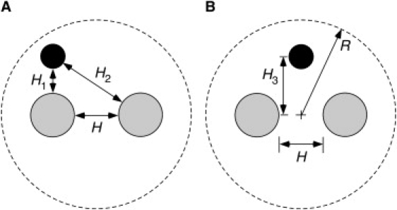
Sphere-fiber systems used to test pairwise additivity of energies: (A) one fiber nearer the sphere; (B) fibers equidistant from the sphere. The dashed circles represent the outer boundaries of the cylindrical domains used in the three-dimensional finite element calculations.

When applying pairwise additivity to the periodic arrangement in Fig. 1, it turned out to be sufficient to consider only seven fibers (the central one and the six nearest neighbors). Including the second layer of 12 fibers altered the value of E by no more than 1%. Referring to the coordinates in Fig. 2, the angular-average Boltzmann factor needed for the flow problem was calculated as

$$\overline{g}\left(\rho \right)=\frac{6}{\pi }\underset{0}{\overset{\pi /6}{\int }}\exp \left[-E\left(\rho ,\theta \right)/kT\right]d\theta \text{.}$$ (26)

Parameters

Whereas the hydraulic permeability (K in Eq. 1) scales as R²/μL, the reflection coefficient is determined by the shape of the velocity profile (i.e., the dimensionless functions that multiply either $d{\overline{P}}_{\text{R}}/dz$ or R_gTdf/dz in Eqs. 15 and 16). The form of the velocity profile depends on α (sphere radius/flow radius), β (fiber radius/flow radius), and the parameters that influence $\overline{g}\left(\rho \right)$. Those include τ (flow radius/Debye length, Eq. 20), q_s (dimensionless sphere charge density, Eq. 21), and q_f (dimensionless fiber charge density, Eq. 22). Also involved is

$$\xi =\frac{{\left(R_{\text{g}}T/F\right)}^2\varepsilon R}{kT},$$ (27)

which arises when E is made dimensionless using the thermal energy. Because the fiber volume fraction (ϕ) is often known experimentally, it is desirable to adopt it as a parameter, replacing β (since ϕ = β²). Thus, the form of the velocity solution, together with dimensional analysis of E, indicates that

$${\sigma }_{\text{o}}={\sigma }_{\text{o}}\left(\alpha ,\varphi ,\tau ,q_{\text{s}},q_{\text{f}},\xi \right)\text{.}$$ (28)

In other words, σ_o depends on six dimensionless groups, as compared with just two for an uncharged system, where σ_o = σ_o(α,ϕ) (6).

Given the number of dimensionless groups, a complete exploration of the parameter space was impractical. Accordingly, we focused on certain conditions which are of physiological interest. Two kinds of fiber matrices were considered. The first (Model 1) is a hypothetical array of GAG chains of varying ϕ. In modeling a GAG chain as a charged fiber, representative values are b = 0.5 nm and Q_f = −0.10 C/m² (12). From Eqs. 3, 4, and 29, a sphere the size of serum albumin (a = 3.6 nm) will be completely excluded by such an array if ϕ > 0.018. Accordingly, with Model 1 we considered only 0 ≤ ϕ ≤ 0.020. The other fiber matrix (Model 2) is the endothelial glycocalyx structure of Zhang et al. (6), which has fibers much thicker than GAG chains. In this case the geometry is specified rather precisely (b = 6 nm, H = 8 nm, R = 10.5 nm, and ϕ = 0.33), but the surface charge density is unknown. Thus, with Model 2 we viewed Q_f as a variable. A range of solute sizes was considered with each model, with bovine serum albumin (BSA) used as a benchmark for charge density. Modeling BSA as a sphere with a = 3.6 nm and a net charge of −20 (13) gives Q_s = −0.020 C/m². Except where noted otherwise, c_∞ = 0.15 M.

Results

Sphere-fiber electrostatic energy

In using pairwise additivity to calculate E for the multifiber system it was necessary to have results for a sphere interacting with a single fiber. When Eqs. 19 and 23 are valid, E is a quadratic function of the surface charge densities (11). This may be expressed as

$$\frac{E}{\xi kT}=A_1{q}_{\text{s}}{q}_{\text{f}}+A_2{q}_{\text{s}}^2+A_3{q}_{\text{f}}^2,$$ (29)

where the coefficients A_i are each functions of α, τ, and the surface-to-surface separation, but are independent of ξ and the charge densities. For this system, the characteristic length used in α, τ, q_s, q_f, and ξ is b (rather than R). The dimensional separation is denoted as h and the dimensionless separation is η = κh. There are nonzero energies for a charged sphere interacting with an uncharged fiber (A₂ > 0) and for an uncharged sphere interacting with a charged fiber (A₃ > 0), because a nearby uncharged object of low dielectric constant will distort the diffuse double layer around a charged object. That will affect its surface potential at constant charge density. However, the additional energy contribution when both objects are charged tends to be dominant (A₁ > A₂ or A₃).

It was shown previously that the results of some 900 three-dimensional finite element calculations for various combinations of inputs could be correlated as

$$A_{\text{i}}\left(\alpha ,\tau ,\eta \right)=a_{\text{i}}{\alpha }^{b_{\text{i}}}{\tau }^{-c_{\text{i}}}\exp \left(-\eta d_{\text{i}}\right),$$ (30)

where a_i, b_i, c_i, and d_i are constants obtained from a least-squares fit (11). The constants reported before are accurate for τα > 0.6, as already mentioned. To improve the results for τα < 0.6, we computed energies for an additional 60 cases with 0.5 < τ < 2, 0.2 < α < 0.6, and 0.1< η < 0.5. A new set of constants for Eq. 30 was obtained by nonlinear least-squares fitting using MATLAB. Those constants represented E well enough to give a root-mean-square error in the Boltzmann factor [exp(−E/kT)] of 10% for τα < 0.6. Both sets of constants are given in Table 1.

Table 1.

Constants for sphere-fiber energy correlation

Range of τα	Index (i)	ai	bi	ci	di
<0.6	1	3.9006	0.7367	0.7814	1.2076
	2	0.276	0.8094	0.4518	2.7655
	3	0.5641	0.9322	0.1699	2.9824
>0.6	1	2.3523	−0.0071	1.2472	1.0956
	2	0.357	0.5436	0.9512	3.7684
	3	0.4473	−0.0822	1.1512	2.4987

When used in Eq. 30, these constants give the electrostatic free energy for double-layer interactions between a sphere and a single fiber (cylinder of indefinite length), each with a constant surface charge density. The results for τα < 0.6 are from this work, whereas those for τα > 0.6 are based on previous results (11).

Pairwise additivity

The assumption that the sphere-fiber energies are pairwise-additive was tested using 60 perpendicular cases (Fig. 3 A), 20 collinear (Fig. 3 B with H₃ = 0), and 18 isosceles (Fig. 3 B with H₃ ≠ 0). In each, the exact Boltzmann factor from the finite element calculation for a sphere and two fibers was compared with that from pairwise additivity. To avoid any errors introduced by Eq. 30, each two-body energy was generated using the same finite element procedure as with the three-body problem. As shown in Fig. 4, for the perpendicular arrangement the agreement between the exact and pairwise Boltzmann factors was remarkably good. The agreement was usually good also for the equidistant configurations (collinear or isosceles), although there were large errors in some cases. When significant errors occurred the pairwise additivity assumption overestimated the Boltzmann factor. By overestimating the ability of a macromolecule to enter the fiber array, this will tend to underestimate σ_o.

Figure 4.

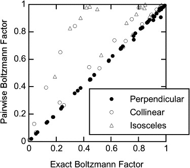
Comparison of exact and pairwise-additive Boltzmann factors [exp(−E/kT)] for a charged sphere interacting with two charged fibers. “Perpendicular” refers to the arrangement in Fig. 3A, and “collinear” and “isosceles” are the configurations in Fig. 3B with H₃ = 0 and H₃ ≠ 0, respectively.

These results suggest that if one fiber is nearest the sphere (which is always true for the perpendicular arrangement in Fig. 3 A), pairwise additivity is a reliable way to correct E for the effects of more distant fibers. Having two or more fibers equidistant from the sphere (as in Fig. 3 B) probably is a worst case, in that no single interaction is dominant. Because a sphere placed randomly within a hexagonal lattice is likely to have only one nearest-neighbor fiber, we conclude that pairwise additivity is a reasonable approximation, at least until a practical alternative can be developed. Incidentally, when the pairwise Boltzmann factors were computed using Eq. 30, the results (not shown) were nearly identical to those in Fig. 4. This indicates that the correlation itself does not introduce significant error in the energy calculations, and that the main concern is the pairwise-additivity assumption.

Osmotic reflection coefficient

We begin with Model 1, which is based on GAG properties. Fig. 5 shows σ_o for BSA as a function of fiber volume fraction (ϕ) for three bulk electrolyte concentrations (c_∞). Higher volume fractions correspond to smaller interfiber spaces, so that in each case σ_o increases with increasing ϕ. For the BSA and GAG radii, complete solute exclusion does not occur until ϕ = 0.018, but σ_o → 1 well before that, depending on the salt concentration. Decreasing the ionic strength (as might be done with biological hydrogels in vitro) increases the Debye length and therefore amplifies the repulsive sphere-fiber electrostatic interactions. Accordingly, at a given ϕ, decreases in c_∞ elevate σ_o. Also shown is a curve for uncharged spheres and fibers with the same radii as BSA and GAG, respectively. The increase in σ_o due to the charge of BSA and GAG is quite significant. For example, at a physiological salt concentration (c_∞ = 0.15 M) and ϕ = 0.005, charge effects are predicted to increase σ_o from 0.30 to 0.87.

Figure 5.

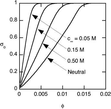
Osmotic reflection coefficient (σ_o) as a function of fiber volume fraction (ϕ) for Model 1 (GAG parameters) and BSA. Results are shown for BSA and GAG at three electrolyte concentrations, and for an uncharged system with the same solute and fiber radii.

The effects of charge vanish as ϕ → 0, and the curves in Fig. 5 all converge at σ_o = 0. With the fiber radius fixed, ϕ → 0 corresponds to a fiber-fiber separation increasing without bound. As the interfiber separation increases, so does the average sphere-fiber separation, and therefore E → 0 for a progressively larger fraction of the possible sphere positions. Thus, electrostatic interactions become unimportant. Likewise, as the sphere centers are excluded from smaller and smaller fractions of the liquid volume, steric effects vanish. As shown by Zhang et al. (6), for a neutral system σ_o → α² as ϕ → 0. For a constant sphere radius, α vanishes along with ϕ, making σ_o zero in that limit.

Over most of the range of ϕ in Fig. 5, our numerical results for the neutral case are within 1% of those obtained from the analytical expression of Zhang et al. (6) (not shown). Noticeable deviations occur only for ϕ > 0.014, the most tightly fitting cases. The analytical expression predicts that σ_o = 1 at ϕ = 0.015, and yields unrealistic values (σ_o > 1) if applied at larger volume fractions; the numerical results for σ_o approach unity asymptotically as ϕ → 0.018 (the absolute steric cutoff). Accounting for the limits on sphere angular position (Eq. 5) is what enables the numerical results to be more realistic for the tightly fitting cases.

Fig. 6 shows the effects of solute radius, again for Model 1. Here, σ_o is plotted as a function of a for several values of ϕ. In each case, the sphere surface charge density is assumed to be that of BSA. As expected, for any constant fiber volume fraction, increasing the solute radius increases σ_o. For a given solute radius, increasing the fiber volume fraction increases σ_o, as shown already for BSA in Fig. 5.

Figure 6.

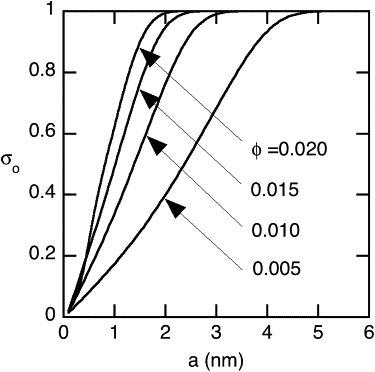
Osmotic reflection coefficient as a function of solute radius (a) for Model 1 (GAG parameters). Curves are shown for four fiber volume fractions, with Q_s = −0.020 C/m² (surface charge density of BSA) in each case.

The effects of solute radius are illustrated again in Fig. 7, this time for Model 2, the endothelial glycocalyx structure of Zhang et al. (6). In this plot the surface charge density is the additional parameter varied, and for each curve it is assumed that Q_s = Q_f = Q. The upper bound chosen for |Q| is that for a GAG fiber. (The absolute value is used because the fibers and solutes are each negatively charged.) It is seen that σ_o increases with a when Q is fixed, and that it increases with |Q| when a is held constant.

Figure 7.

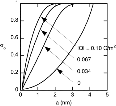
Osmotic reflection coefficient as a function of solute radius for Model 2 (endothelial glycocalyx parameters). Results are shown for four sphere and fiber charge densities, with Q_s = Q_f = Q.

An aspect of Model 2 mentioned earlier is that the fiber charge density is unknown. Fig. 8 shows σ_o for this model as a function of |Q_f| for several values of |Q_s|, with the solute size fixed at a = 3.6 nm (as for BSA). Whether |Q_f| and |Q_s| are elevated separately or in combination, σ_o is increased above its fully neutral value of 0.68. The different σ_o intercepts at |Q_f| = 0, and the increasing trend seen in the curve for |Q_s| = 0, each reflect the fact that electrostatic interactions exist even if only one object is charged (Eq. 29).

Figure 8.

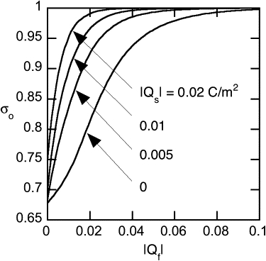
Osmotic reflection coefficient as a function of fiber charge density (|Q_f|) for Model 2 (endothelial glycocalyx parameters). Curves are shown for four sphere charge densities (|Q_s|).

The largest solute charge density shown in Fig. 8 corresponds to that of BSA. Serum albumins are highly retained in the circulation, with σ_o > 0.9 typically. Such high selectivity is not predicted for BSA and neutral fibers, where σ_o = 0.75 in Fig. 8 (somewhat above the fully neutral value of 0.68). It is seen that a fiber charge density of only −0.01 C/m² is required to make σ_o > 0.9. This is only one-half the charge density of BSA or one-tenth that of a GAG chain. This suggests that, with realistic fiber charge densities, the endothelial glycocalyx alone might be capable of retaining albumin with the efficiency typically observed in normal capillaries.

Discussion

A computational model was developed to predict the osmotic reflection coefficient for charged, spherical, macromolecules in membranes consisting of regular arrays of charged fibers. To obtain a tractable problem, we assumed that the fibers are arranged in a hexagonal array and that flow is parallel to the fiber axes, as in the analysis in Zhang et al. (6) of osmosis in an uncharged system. Whether charge is present or not, the underlying mechanism for osmotic flow in these models is that proposed by Anderson and Malone (9) for porous membranes. That is, steric and/or electrostatic exclusion of solute centers from the vicinity of fiber surfaces (or pore walls) creates concentration-dependent variations in mechanical pressure in the transverse direction. When there is a concentration difference imposed across the membrane, this leads to axial gradients in mechanical pressure that result in osmotic flow. When solutes and fibers are of like charge and have constant surface charge densities, solute-fiber electrostatic interactions are always repulsive. These electrostatic interactions are longer range than purely steric ones. Hence, there is increased exclusion of macromolecular solutes from the membrane, and σ_o with charge effects always exceeds that for an otherwise identical, neutral system. The osmotic reflection coefficient becomes a function then not only of solute size, fiber size, and fiber volume fraction, but also solute charge density, fiber charge density, and electrolyte concentration. The factors that affect σ_o are stated more precisely in Eq. 28, which lists all the pertinent dimensionless groups.

Perfectly selective exclusion of solute molecules is the defining feature of an ideal, semipermeable membrane, where σ_o = 1; failure to discriminate between solute and solvent molecules precludes osmosis, in which case σ_o = 0. Accordingly, σ_o is related to the partition coefficient (Φ), which is the solute concentration in the membrane relative to that in bulk solution, at equilibrium. For hydrogels or other fibrous media, it is conventional to base the intramembrane concentration on total volume (solid plus liquid). Accordingly, for the fiber array modeled here (Fig. 2),

$$\Phi =\frac{12}{\pi }\underset{0}{\overset{\pi /6}{\int }}\underset{\alpha +\beta }{\overset{1}{\int }}\exp \left[-E\left(\rho ,\theta \right)/kT\right]\rho d\rho d\theta \text{.}$$ (31)

The relationship between σ_o and Φ is examined in Fig. 9, where each point represents a combination of parameter values considered in Figs. 5–8. The abscissa, Φ/(1 − ϕ), corresponds to a partition coefficient in which intramembrane concentrations are based on liquid volume, as for porous membranes. Even with this adjustment for fiber volume fraction, the results follow two different relationships, one corresponding to Model 1 (ϕ << 1) and the other Model 2 (ϕ = 0.33). This is in contrast to what has been found for porous membranes, where all results for a given pore shape tend to scatter about a single curve (3–5,9). (The relationships differ somewhat depending on pore shape, and the scatter for a given shape is much less if charge effects are absent.) If the abscissa had been Φ (partitioning based on total volume), the two sets of points in Fig. 9 would have been separated much more.

Figure 9.

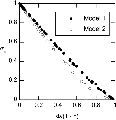
Relationship between osmotic reflection coefficient and equilibrium partition coefficient (Φ). The abscissa corresponds to a partition coefficient that has been adjusted using the fiber volume fraction (ϕ) to base intramembrane concentrations on liquid volume. Each point corresponds to a set of parameter values from Figs. 5–8, with solid symbols from Model 1 and open symbols from Model 2.

We conclude from Fig. 9 that, for charged solutes and charged fibrous membranes, there is not a universal relationship between σ_o and Φ. The absence of such a relationship is evident also in the analytical results of Zhang et al. (6) for neutral solutes and fibers, where Φ depends only on α + β, but σ_o is a complicated function of α and β separately. (The neutral result, Φ = 1 – (α + β)², follows from Eq. 31 by setting E = 0 and ignoring the angular restriction expressed in Eq. 5.)

The main difficulty encountered was how to evaluate the electrostatic free energy (E) for a sphere interacting with a hexagonal array of fibers of indefinite extent. Because of the three-dimensional geometry and the need to resolve details of the potential over distances often much smaller than the fiber-fiber separation, direct finite element solutions of Eq. 19 for a sphere interacting with many fibers were not feasible. In preliminary calculations we explored the singularity method of Phillips (14), which is well suited for solving Eq. 19 in settings where boundary conditions must be imposed on the surfaces of multiple objects. Although we found this method to work well for certain test cases (e.g., a pair of spheres), our ability to satisfy the constant charge density boundary conditions turned out to be very sensitive to the placement of the internal singularities and the selection of surface points. Because it was impractical to optimize the singularity method for each of the many asymmetrical sphere positions we had to consider, we abandoned it in favor of a pairwise-additivity assumption for the energies.

Pairwise additivity, when combined with a correlation for the interaction energy between a sphere and a single fiber (Eq. 30), was straightforward to implement. As shown in Fig. 4, Boltzmann factors calculated using pairwise additivity, although imperfect, were usually reliable in tests involving a sphere and two fibers. When significant errors occurred, there was a tendency to overestimate the Boltzmann factor, which in turn would overestimate Φ and underestimate σ_o. In that sense, the predicted increases in σ_o due to charge are conservative. Although the accuracy of the σ_o results would be improved if E could be computed more precisely, we think it unlikely that any of the plots would change a great deal.

For both types of fiber arrays considered, one based on the properties of GAG chains and the other corresponding to the endothelial surface glycocalyx model of Zhang et al. (6), σ_o for BSA was predicted to be much larger than that for a neutral system (Figs. 5 and 8). Thus, whether one envisions a capillary wall as having a barrier like that of Model 1 or Model 2, this suggests that charge is important in minimizing albumin loss from the circulation. This conclusion is based on the equality (or near equality) of σ_o and σ_f and the assumption that minimizing convective transport through capillary walls is important for retaining albumin.

Of course, an array of GAG chains is unlikely to be as highly ordered as assumed in Fig. 1, and even so, the flow may not be parallel to the fibers. It would be worthwhile to extend this type of model to flow that is perpendicular to an array of fibers. The results for the parallel and perpendicular problems might then be combined to predict σ_o for arrays of randomly oriented fibers, perhaps using mixing rules analogous to those used to estimate the hydraulic permeability of such arrays (12).

References

- 1.Deen W.M. Hindered transport of large molecules in liquid-filled pores. AIChE J. 1987;33:1409–1425. [Google Scholar]
- 2.Levitt D.G. General continuum analysis of transport through pores. I. Proof of Onsager's reciprocity postulate for uniform pore. Biophys. J. 1975;15:533–552. doi: 10.1016/S0006-3495(75)85836-X. [DOI] [PMC free article] [PubMed] [Google Scholar]
- 3.Anderson J.L. Configurational effects of the reflection coefficient for rigid solutes in capillary pores. J. Theor. Biol. 1981;90:405–426. [Google Scholar]
- 4.Bhalla G., Deen W.M. Effects of molecular shape on osmotic reflection coefficients. J. Membr. Sci. 2007;306:116–124. [Google Scholar]
- 5.Bhalla G., Deen W.M. Effects of charge on osmotic reflection coefficients of macromolecules in porous membranes. J. Colloid Interface Sci. 2007;333:363–372. doi: 10.1016/j.jcis.2009.01.019. [DOI] [PubMed] [Google Scholar]
- 6.Zhang X., Curry F.-R., Weinbaum S. Mechanism of osmotic flow in a periodic fiber array. Am. J. Physiol. 2006;290:H844–H852. doi: 10.1152/ajpheart.00695.2005. [DOI] [PubMed] [Google Scholar]
- 7.Dechadilok P., Deen W.M. Hindrance factors for diffusion and convection in pores. Ind. Eng. Chem. Res. 2006;45:6953–6959. [Google Scholar]
- 8.Happel J. Viscous flow relative to arrays of cylinders. AIChE J. 1959;5:174–177. [Google Scholar]
- 9.Anderson J.L., Malone D.M. Mechanism of osmotic flow in porous membranes. Biophys. J. 1974;14:957–982. doi: 10.1016/S0006-3495(74)85962-X. [DOI] [PMC free article] [PubMed] [Google Scholar]
- 10.Verwey E.J.W., Overbeek J.T.G. Elsevier; Amsterdam, The Netherlands: 1948. The Theory of the Stability of Lyophobic Colloids. [Google Scholar]
- 11.Johnson E.M., Deen W.M. Electrostatic effects on the equilibrium partitioning of spherical colloids in random fibrous media. J. Colloid Interface Sci. 1996;178:749–756. Erratum in J. Colloid Interface Sci. 1997. 195:268. [Google Scholar]
- 12.Mattern K.J., Nakornchai C., Deen W.M. Darcy permeability of agarose-glycosaminoglycan gels analyzed using fiber mixture and Donnan models. Biophys. J. 2008;95:648–656. doi: 10.1529/biophysj.107.127316. [DOI] [PMC free article] [PubMed] [Google Scholar]
- 13.Vilker V.L., Colton C.K., Smith K.A. The osmotic-pressure of concentrated protein solutions—effect of concentration and pH in saline solutions of bovine serum albumin. J. Colloid Interface Sci. 1981;79:548–566. [Google Scholar]
- 14.Phillips R.J. Calculation of multisphere linearized Poisson-Boltzmann interactions near cylindrical fibers and planar surfaces. J. Colloid Interface Sci. 1995;175:386–399. [Google Scholar]