RazerS—fast read mapping with sensitivity control

Abstract

Second-generation sequencing technologies deliver DNA sequence data at unprecedented high throughput. Common to most biological applications is a mapping of the reads to an almost identical or highly similar reference genome. Due to the large amounts of data, efficient algorithms and implementations are crucial for this task. We present an efficient read mapping tool called RazerS. It allows the user to align sequencing reads of arbitrary length using either the Hamming distance or the edit distance. Our tool can work either lossless or with a user-defined loss rate at higher speeds. Given the loss rate, we present an approach that guarantees not to lose more reads than specified. This enables the user to adapt to the problem at hand and provides a seamless tradeoff between sensitivity and running time.

Second-generation sequencing technologies are revolutionizing the field of DNA sequence analysis, as large amounts of sequencing data can be obtained at increasing rates and dramatically decreasing costs. Biological applications are manifold, including whole-genome resequencing for the detection of genomic variation, e.g., single nucleotide polymorphisms (SNPs) (Bentley et al. 2008; Hillier et al. 2008; Ley et al. 2008; Wang et al. 2008) or large structural variations (Chen et al. 2008), RNA sequencing for small noncoding RNA discovery or expression profiling (Morin et al. 2008), metagenomics applications (Huson et al. 2007), and sequencing of chromatin-immunoprecipitated DNA, e.g., for the identification of DNA binding sites and histone modification patterns (Barski et al. 2007).

Fundamental to all these applications is the problem of mapping all sequenced reads against a reference genome, denoted as the read mapping problem. It can be formalized as follows: given a set of read sequences , a reference sequence G, and a distance , find all substrings g of G that are within distance k to a read . The occurrences of g in G are called matches. Common distance measures are Hamming distance or edit distance; the former forbidding insertions and deletions (i.e., indels) in the alignment, the latter allowing for mismatches and indels alike.

As the new sequencing technologies are able to produce millions of reads per run, efficient algorithms for read mapping are necessary. Reads are typically quite short compared to the traditional Sanger reads and have specific error distributions depending on the technology used.

A variety of tools have been designed and developed specifically for the purpose of mapping short reads. A compilation of some popular tools is shown in Table 1 together with some key features of the algorithms.

Table 1.

Short read mapping tools with their characteristics

Most of the existing read mapping approaches use a two-step strategy. First, a filtration algorithm is applied in order to identify candidate regions that possibly contain a match. This includes building an index data structure, either on the set of reads or on the reference sequence. Second, candidate regions are examined for true matches in a more time-consuming verification step. In current implementations one has to carefully distinguish whether both steps, the filtration step and the verification step, are adequate for the distance chosen (Hamming or edit distance). Some implementations, for instance, verify matches using base-call qualities, but filter the candidate regions using a fixed Hamming or edit distance (H Li et al. 2008). Filtration methods in use are based on single (Kent 2002; Ma et al. 2002) or multiple seeds (Li et al. 2003; Lin et al. 2008), the pigeonhole principle (Navarro and Raffinot 2002; H Li et al. 2008; R Li et al. 2008; AJ Cox, ELAND: Efficient local alignment of nucleotide data, unpubl.), or based on counting lemmas using (gapped) q-gram (Burkhardt et al. 1999; Rasmussen et al. 2006; Rumble and Brudno 2008). Verification methods encompass semiglobal alignment algorithms for Hamming or edit distance (Levenshtein 1966) or local-alignment algorithms (Smith and Waterman 1981).

BLAT (Kent 2002), as an example of a single seed filter, searches exact occurrences of short fixed sized substrings shared by two sequences. PatternHunter (Ma et al. 2002) was the first to generalize this strategy to gapped seeds (common discontiguous subsequences), thereby increasing sensitivity while maintaining specificity. Further sensitivity is achieved by using multiple gapped seeds; an approach implemented in the read mapping tool Zoom (Lin et al. 2008), which uses a restricted version of edit distance with at most one gap. After the initial submission of this paper a method using whole reads as seeds was published, which tolerates a small number of mismatches by backtracking all possible replacements of low-quality bases (Langmead et al. 2009). It uses Burrows-Wheeler transformed genomes and is an efficient approach to short read mapping.

Given two sequences within distance k, the pigeonhole lemma states that of any partition of the first sequence into k + 1 parts, at least one part must be found without errors in the other sequence. The shorter this seed, the more likely it is to encounter random matches, and therefore the lower the specificity of the filter. This strategy is thus rather limited and quickly grows impractical with an increasing number of errors. In an extension of this strategy the first sequence is divided into k + 2 parts. Now at least two of such parts will occur in the other sequence. These two parts retain their relative positions as long as no indels occur in between. ELAND (AJ Cox, unpubl.), MAQ (H Li et al. 2008), and SOAP (R Li et al. 2008) make use of this observation but are therefore limited to Hamming distance. Furthermore, ELAND and SOAP always use a four-segment partition and MAQ at most a five-segment partition and can therefore not guarantee full sensitivity for k > 2 or k > 3, respectively. SeqMap (Jiang and Wong 2008) extends the two-seed pigeonhole strategy to edit distance and searches the two parts varying the gap length by −k,…, k nucleotides.

Another approach is the q-gram counting strategy which was first used in QUASAR (Burkhardt et al. 1999). It uses the q-gram lemma (Owolabi and McGregor 1988; Jokinen and Ukkonen 1991), which states that two sequences of length n with Hamming distance k share at least t = n + 1 − (k + 1)q common substrings of length q, so-called q-grams. This lemma can also be applied to edit distance if n is the length of the larger sequence. A generalization for gapped q-grams was given by Burkhardt and Kärkkäinen (2002). SHRiMP (Rumble and Brudno 2008) employs a q-gram counting strategy with a default configuration that does not guarantee to be lossless.

In this work we present an implementation of a versatile read mapper RazerS based on q-gram counting, which distinguishes itself in several respects from existing algorithms. First, it can map reads using edit or Hamming distance in the filtering phase and in the verification phase without any restrictions. Second, given a user-defined loss rate (possibly 0 making the mapper exact), we developed an algorithm to select parameters such that the chosen loss rate is not exceeded in expectation. The algorithm depends on an error model derived from base-call quality values. Finally, our implementation can map reads of any length with an arbitrary number of errors and is currently the fastest in reporting all hits for typical read lengths and loss rates.

Methods

Definitions and notation

We consider strings over the finite ordered alphabet Σ. Σ* is the set of all possible strings over Σ and ε denotes the empty string. A string s is a sequence of letters s[1]…s[n], where each s[i] ∈ Σ; st is the concatenation of two strings s and t; |s| denotes the length of the string s; and s[i..j] is a substring of s from position i to j. If t ∈ Σ* is a substring of s, we write t ≼ s, and t ≺ s if t ≠ s holds in addition.

A(n) (edit) transcript is a string over the alphabet Δ = {M, R, D, I} that describes a transformation from one string to another, see Figure 1. For two strings r,g ∈ Σ*, a transcript from r to g is read and applied from left to right to single characters of r to produce g, whereby M, R, D, and I correspond to a match (no change), a replacement, a deletion, and an insertion of a single character in r, respectively. There is a one-to-one relation between alignments and transcripts. For any transcript T we define ||T||_E = |{i|T[i] ∈ {R, D, I}}|, the number of errors in T. The edit distance of two strings is the minimum number of errors in all transcripts between these strings. A special case is the Hamming transcript with Δ = {M, R}. It is defined uniquely for two strings of equal length and the Hamming distance is the number of errors in it.

Figure 1.

A transcript from a read to a part of the genome. The transcript contains seven three-matches, hence r and g share at least seven 3-gram. Actually, they also share an eighth 3-gram CAG that does not correspond to a three-match of the transcript.

In the following we consider transcripts from reads r ∈ to substrings g of a genome G. We say that the pair (r,g) is a true match if d(r,g) ≤ k, for d being either edit or Hamming distance. A substring M^q of a transcript T is called a q-match. If a transcript from r to g contains t q-matches, then r and g have at least t common q-grams. A (q,t)-filter is an algorithm that detects any pair (r,g) for which a transcript T from r to g with ≥t q-matches exists.

Sensitivity calculation

In this section we devise a method to determine the sensitivity of (q,t) filters. The sensitivity of a filter is the probability that a randomly chosen true match (r,g) is classified by the filter as potential match. Existing sensitivity estimation approaches are limited to multiple seed filters (Li et al. 2003) or assume transcripts to be generated by a Markov process (Herms and Rahmann 2008). Our method estimates the filtration sensitivity under any position-dependent error distribution, e.g., as observed in Sanger or Illumina DNA sequencing technologies (Dohm et al. 2008).

Hamming distance sensitivity

We first consider the read mapping problem for Hamming distance and a given maximum distance k. In the following, all reads are considered to be of equal length n.

To determine a lower bound for the sensitivity of a (q,t)-filter we could enumerate all Hamming transcripts with up to k replacements and sum up the occurrence probabilities of those transcripts having at least t substrings M^q. As there are many different transcripts, a full enumeration takes Ω[(n/k)^k] time and is not feasible for large reads or high error rates, e.g., of length n = 200 with k = 20 errors. We have developed a dynamic programming approach that is significantly faster by using a recurrence similar to the threshold calculation in Burkhardt and Kärkkäinen (2002).

Assume a given error distribution that associates each nucleotide position i in a read with an error probability P_i^R, e.g., the probability of a base miscall during sequencing or a SNP. Then, the occurrence probability of a Hamming transcript T is the product of the occurrence probabilities of the single transcript characters at each position p(T) = , with . We calculate the sensitivities for matches with e errors for each e ≤ k separately. Let S(n, e, t) be the sum of occurrence probabilities of transcripts of length n, having e errors, and at least t q-matches. The sensitivity of a (q,t)-filter to detect e-error matches is at least

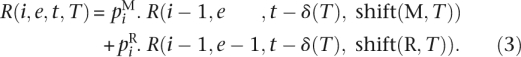
We will see, how to calculate S(n, e, t) using a DP algorithm. Let 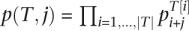be the occurrence probability of subtranscript T to occur after j letters of a read. We define R(i, e, T₂) as the sum of occurrence probabilities of transcripts T_i ∈ Δ^I, so that T₁ has e errors and the concatenation T₁T₂ contains at least t substrings M^q. By definition of S holds:

The sum goes over all transcript ends T of length q with at most e errors. The right factor is the probability of T occurring at the end of a random transcript of length n. The left factor is the occurrence probability sum over all transcript beginnings, so that the concatenation of beginning and end is a transcript of length n with e errors, and at least t q-matches. With the following lemma a DP algorithm can be devised to determine R and therefore the sensitivities S(n, e, t) for all e = 0, …, k and t = 1, …, t_max in (nkt_max2^q).

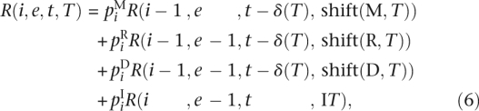
Lemma 1. Let i, q ∈ ; e, t ∈ ; T ∈ {M, R}^q. R can be calculated using the following recurrence:

with

Proof. See Appendix.

Extension to gapped shapes

A generalization of contiguous q-grams are gapped q-grams (Burkhardt and Kärkkäinen 2002), (noncontiguous) subsequences of length q. A shape Q is defined to be a set of non-negative integers corresponding to nongapped positions, where 0 ∈ Q is the first nongapped position. For example, the 3-gram of shape ##-# in the string GTTCA are GTC and TTA and the corresponding shape is Q = {0, 1, 3}. The span of Q is span(Q) = max Q + 1 and the weight of Q is the set cardinality |Q|. For any integer i we define Q_i = {i + j|j ∈ Q}. Let Q_i = {i₁, …, i_|Q|}, where i = i₁ < i₂ < … < i_|Q| and s be a string. For 1 ≤ i ≤ |s| − span(Q) + 1, s[Q_i] is defined to be the string s[i₁]s[i₂]…s[i_|Q|] and called Q-gram at position i. Contiguous q-grams are Q-grams with the shape Q = {0, 1,…, q − 1}.

A Q-gram M^|Q| of a Hamming transcript T is called a Q-match, and a (Q t)-filter is an algorithm that detects any pair (r,g) for which a transcript T from r to g with ≥t Q-matches exists. To extend the sensitivity calculation to gapped shapes Q, the transcript T in Lemma 1 must be resized to cover the whole shape and the matching criterion in δ(T) must be adapted. This can be done by replacing q in Equation 1 by span (Q) and δ(T) in Equations 2 and 3 by

For two strings of length span(Q) with the Hamming transcript T ∈ Δ^span(Q), δ(T) returns 1 if and only if they share their sole Q-gram. A lemma similar to Lemma 1 can be proven analogously.

Edit distance sensitivity

We extended the sensitivity calculation to edit distance. The DP algorithm and the proof of correctness can be found in the Appendix.

The algorithm

In the following, we propose the read mapping algorithm implemented in RazerS. It consists of three parts: a parameter chooser, a filter, and a verifier.

Filtration

To find potential match regions of reads in the genome we use the SWIFT algorithm (Rasmussen et al. 2006). It incorporates the following two observations. Consider an edit transcript between two sequences with at least t q-matches. First, the dot plot of the sequences contains at least t contiguous diagonal lines of length q, so called q-hits. Second, if the transcript contains k errors then there are k + 1 consecutive diagonals covering at least t q-hits. In case of Hamming transcripts, there is a single diagonal completely covering all q-hits.

For any read r ∈ each dot plot parallelogram of dimension |r| × (k + 1) with at least t q-hits contains a potential match. Instead of counting q-hits for each possible parallelogram separately, it suffices to count them in overlapping |r| × w parallelograms with w > k + 1 and an overlap of k, as every |r| × (k + 1) parallelogram is contained in one |r| × w parallelogram, see Figure 2.

Figure 2.

The dot plot between a read and a genome is covered by parallelograms that span w = 12 diagonals and overlap by k = 4 diagonals. Common 3-gram are counted for each parallelogram. The marked parallelogram contains the complete transcript, therefore it counts all 3-gram that correspond to the seven three-matches in the transcript.

If for i,j ∈ holds r[i..i + q − 1] = G[j..j + q − 1], the corresponding q-hit is covered by the diagonal j − i. For an overlap of k and w = d + k the |r| × w parallelograms begin at diagonals 0, d, 2d,… . If d is a power of 2, the parallelograms containing a q-hit can efficiently be determined by bit-shifting j − i.

q-Hits are determined by searching overlapping q-grams G[j..j + q − 1], j = 1,… , |G| − q + 1 in a q-gram index of all overlapping q-grams of sequences in . Only a small number of counters are needed per read, when sliding the q-gram over G. As every |r| + w parallelogram spans at most |r| + w − 1 letters of G, a parallelogram counter can be re-used after |r| − w − q sliding steps. Before re-using a counter, the associated parallelogram is verified if the counter has reached threshold t.

The SWIFT approach can also be used with gapped shapes Q using a Q-gram index and replacing each q in the formulas above by span(Q).

Verification

To verify a parallelogram possibly containing a true match with edit distance less or equal k, we use Myers (1999) bit-vector algorithm. It exploits hardware parallelism of bit-operations. A 64-bit CPU can calculate 64 cells of the edit matrix at once in a constant number of 14 arithmetic operations.

If r ∈ and g ≺ G are the strings covered by a parallelogram of the previous step, it calculates for each j = 1,…, |g| the minimal edit distance between r and all substrings of g ending at position j. If for a position j the minimal edit distance is less or equal to k, a true match is found ending at j. With a slight modification of the algorithm, g[1..j] can be searched for a beginning position i of the true match. Finally, (r,g[i..j]) is recorded as a true match.

If only Hamming matches are considered, a parallelogram is verified by scanning each diagonal character by character until more than k mismatches occur. A diagonal d corresponding to r ∈ and G[d + 1..d + |r|] with less or equal k mismatches covers the true match (r,G[d + 1..d + |r|]).

Choosing filtration parameters

We now want to automatically choose filtering parameters, a shape Q, and a threshold t, such that (1) we achieve a certain sensitivity level and (2) the running time of the mapping procedure is minimized.

For all read lengths from 24 to 100 and error rates up to 10%, we have therefore precomputed the sensitivities using a number of different shapes and thresholds. As an error distribution we assume a typical Illumina error profile (Dohm et al. 2008). Additionally, all parameter combinations were used to run RazerS on simulated data, yielding a rough estimate for the corresponding filtration efficiency. Parameters for reads longer than 100 base pair (bp) are extrapolated from parameters of precomputed shorter reads with the same error rate. Given a user-defined minimum sensitivity, suitable filtration parameters are chosen from the precomputed tables, such that the anticipated running time is minimized.

If preferred, the parameter tables can be precomputed based on a machine-specific error distribution and user-defined shapes. This error distribution can be obtained in two ways. (1) Quality-based probabilities: Transform the average base-call quality value for each position into a probability value. (2) A posteriori probabilities: Map a small subset of reads and determine the position-dependent error frequency. Given an error distribution the parameters for reads of length 50 can, for instance, be calculated within 10 min.

Results and Discussion

In this section, we empirically verify the above-described calculation of the expected mapping sensitivity and compare the performance of our tool to that of other read mappers. We use simulated as well as real data. The real data sets were all downloaded from the NCBI Short Read Archive (http://www.ncbi.nlm.nih.gov/Traces/sra/):

• The first set (run accession SRR001815) comprises 10,760,364 Drosophila melanogaster reads of length 36 bp.

• The second set (run accession SRR006387) contains 2 × 7,894,743 76 bp paired-end reads obtained from whole genome shotgun sequencing of a human HapMap individual, which we trimmed to the first 63 bp (the maximal read length of Zoom at the time of writing).

In both sets, the Illumina technology was used. As references we used the RepeatMasker (http://www.repeatmasker.org) versions of the D. melanogaster genome from FlyBase (http://www.flybase.org/), Release 5.9, and the human genome from NCBI (http://www.ncbi.nlm.nih.gov/), Build 36.3.

Verification of expected sensitivity

We verify the correctness of our sensitivity estimation by assessing the discrepancy between estimated and empirical sensitivity for the following two scenarios, where the first one serves as a sanity check:

1. Simulated data. We simulate DNA sequence reads using position-dependent error probabilities and group them according to the number of implanted errors. After mapping the reads to the reference sequence, we define the empirical sensitivity for each group as the proportion of reads that could be mapped back to their genomic origin. Using the same error distribution as for simulation, we compute the estimated sensitivity as described above.

2. Real data. We map the set of reads once with 100% sensitivity and keep as reference matches only those reads that map uniquely. Again, we group them according to the number of errors and determine the empirical sensitivity as for simulated data. The expected sensitivity is computed using the a posteriori probabilities (see previous section).

Using these two protocols, we examined mapping sensitivity for simulated 36 bp reads and for a subset of the 36 bp reads in SRR001815. We inspected both Hamming as well as edit distance sensitivity and did the mapping for all ungapped shapes of weight q where 8 ≤ q ≤ 14 and all thresholds t where 1 ≤ t ≤ 20.

As a measure of accuracy we use the relative difference between empirical and estimated loss rate. We observe a very good agreement for Hamming distance (see Fig. 3). For expected loss rates between 0 and 10% the mean relative difference for simulated, as well as real data, is below 0.1%. Considering edit distance, the expected loss rates overestimate the empirical loss. Between 0 and 10% of expected loss the mean relative difference is below 4% for simulated and below 2.8% for real data. For edit distance the SWIFT parallelograms are broader and produce more random q-gram hits compared to Hamming distance mapping, where the parallelograms are single diagonals. This leads to more matches than expected. The discrepancy for simulated data is slightly more pronounced. This can be explained by the observation that simulated matches are not necessarily optimal, i.e., reads can be mapped with less error than originally implanted (e.g., an insertion next to a deletion will be aligned as one replacement). Most notably, in all cases the empirical sensitivities are higher than expected, thereby yielding better mapping results than estimated.

Figure 3.

Comparison of estimated and empirical loss rates (loss rate = 1 − sensitivity) varying weight q = 8,…, 14 and threshold t = 1,…, 20. The dashed line reflects the mean of relative differences, 1 − (empirical loss rate/estimated loss rate), of all estimated loss rates below a varying level.

Furthermore we investigated the distribution of the lost reads. We therefore compared the output of the 99% with the 100% sensitivity mapping of all Drosophila reads onto the Drosophila genome and observed a uniform distribution of lost reads over the whole genome. For example, of all 224,229 nonoverlapping 100 bp bins of chromosome X, 199,029 contained at least one mapped read. A percentage (1.14%) of these bins lost one or more reads when mapping with 99% sensitivity. Of all affected bins, only 2.38% lost more than one and 0.22% more than two reads. More than three reads were never lost. We observed similar values for all the other chromosomes.

Runtime comparisons

We demonstrate the performance of RazerS in comparison to five other read mapping tools: MAQ (H Li et al. 2008), SeqMap (Jiang and Wong 2008), SHRiMP (Rumble and Brudno 2008), SOAP (R Li et al. 2008), and the closed-source, commercial Zoom (Lin et al. 2008). We do not consider ELAND (AJ Cox, unpubl.), as we want to map reads longer than 32 bp and only have access to a version limited to 32 bp reads.

All tools differ in some aspects making the comparison rather difficult. MAQ, for example, has a different objective, minimizing the sum of mismatching quality values instead of minimizing the number of mismatches. Also the treatment of N (unknown base) or how many hits per read can be reported is different from tool to tool. We tried to be as fair as possible by using comparable program configurations. In addition, the comparisons should be understood as a means to give the user an impression of the capabilities of RazerS and not as a comprehesive comparison of read mapping tools. All experiments were conducted on an AMD Opteron 2.8 GHz machine with 64 GB of RAM.

Short reads

1. Drosophila, Hamming distance 2. In the first experiment we mapped the Drosophila read set SRR001815 onto the Drosophila genome with up to two mismatches and measured runtime and space consumption of each read mapping tool. RazerS was run with full sensitivity and with 99% sensitivity. All tools were configured to tolerate two mismatches and output, at most, one best match per read. Since SHRiMP uses a Smith-Waterman verifier, we had to adapt the scoring parameters (mismatch = 0, match = 1, gap penalties = −1000, score threshold = 32).

2. Drosophila, edit distance 2. In this experiment the same set of reads was mapped with up to two errors, allowing mismatches and also indels. Since SHRiMP computes local alignments, there is no scoring scheme for semiglobal edit distance alignments. Nevertheless, we tried to emulate edit distance (mismatch = −1, match = 1, gap penalties = −1, score threshold = 32).

3. Human, Hamming distance 5. For the last experiment on real data we used the first mate set SRR006387 containing 76 bp reads, which we trimmed to 63 bp to incorporate Zoom in our tests. All tools were configured to tolerate five mismatches and output at most one best match per read. Although according to the manual the longest acceptable read length of SOAP is 60 bp, it was capable to match reads of length 63 bp without simply trimming the reads. We tried to run Zoom with 100% sensitivity using the “-sv r5” option, which resulted in an error message, so we reduced Zoom to be fully sensitive for four error matches (r4). For SHRiMP we again adapted the scoring parameters as in Experiment 1 with scoring threshold = 58.

The results are summarized in Table 2. Clearly, reducing the sensitivity by 1% has a notable influence on runtime. In Experiment 2 the runtime could be reduced by a factor of 2 and for larger reads in Experiment 3 even by a factor of 13. RazerS99 outperforms the other read mapping tools in almost all experiments and has comparable memory consumption. The runtimes for mapping with Hamming distance are up to 16 times less compared to edit distance. This can be explained by the more efficient Hamming verification algorithm and the observation that gapped shapes, which are chosen for Hamming distance, improve the filtration specificity and runtime. For edit distance, gapped shapes are often less sensitive than their corresponding ungapped shape of equal weight with a smaller span, as indels harm a gapped shape along the whole span.

Table 2.

Short read results

Results for mapping 1,000,000 and 10,760,364 (all) reads of length 36 bp onto the Drosophila genome allowing for two errors considering Hamming (1) or edit distance (2) and for mapping 1,000,000 and 7,894,743 reads of length 63 bp onto the human genome allowing for five replacement errors (3). The fastest method is marked in bold.

^aSOAP and MAQ do not support edit distance and MAQ also reports matches with more errors (quality based matching).

The numbers of mapped reads are similar across the different read mapping tools. In all experiments RazerS99 recognizes 99.62%–99.87% of the matches found by RazerS100. Zoom finds less matches than RazerS100 in experiments (2) and (3) because it recognizes matches with at most one contiguous gap and is not fully sensitive for five errors. SeqMap loses matches partially covering reference regions consisting of N's. SHRiMP's q-gram filter is lossless only for Experiment 3 and reports additional matches because it matches N with N, which are discarded by RazerS. SOAP maps all masked or unknown bases N to A and thus reports more matches. As MAQ uses a quality-based match verification (minimizing the sum of mismatch qualities) it finds matches with more errors, shown in brackets. To make the results comparable, we counted only matches with at most two or five mismatches. The matches not found by MAQ are those having more than three mismatches in the first 28 bp prefix and those that are discarded for a match with more errors and a lower sum of mismatch quality values.

Paired-end reads

RazerS is also capable of mapping paired-end reads.We therefore scan the reference genome from left to right in parallel with two SWIFT filters having the distance of the library size minus a tolerated library size deviation. Each filter searches for potential matches of one of the two ends of all pairs. Additionally, we record in a queue all matches of the left filter within a distance of the doubled tolerated library size deviation. Only if the right filter finds a potential match whose mate potential match is stored in the queue both potential matches are verified. This guarantees that verifications are only done if both potential matches are within the correct distance.

To compare the paired-end alignment performance of RazerS with other paired-end aligners and also to see the behavior of the tools on unmasked reference sequences, we mapped the trimmed SRR006387 set of 2 × 63 bp paired-end reads onto the unmasked human chromosome 21 with up to five mismatches per mate, a library size of 200 bp, and a tolerated library size error of 50 bp. Paired-end alignment is supported by MAQ, SOAP, and Zoom, however, SOAP is limited to two mismatches and therefore left out of this comparison. All tools were run with the same options as in Experiment 3 adding the corresponding paired-end options.

Table 3 shows the results. We observe a runtime decrease by a factor of five between full and 99% sensitivity. Compared to Experiment 3 this factor is lower due to the library length criteria, which prevents costly verifications of matches outside the tolerated library size independent of the chosen sensitivity. Zoom is the fastest but also the least sensitive tool. We suspect that the sensitivity option (“-sv r4”) is not applicable to paired-end reads. Of all pairs mapped by MAQ within the tolerated library size (values shown in parentheses) we counted those having up to five errors. The smaller number of mapped pairs can be explained as above.

Table 3.

Results for mapping 2 × 1,000,000 and 2 × 7,894,743 paired-end reads of length 63 bp onto the unmasked human chromosome 21, allowing for five replacement errors per read

The fastest method is marked in bold.

Large reads

To demonstrate that our approach is also applicable to larger reads, we simulated 500,000 reads of lengths 125 and 250 bp of the unmasked human chromosome 21 and implanted up to 10 and 20 errors under a widened Illumina error profile (Dohm et al. 2008). Only RazerS and SHRiMP were able to map both and MAQ was able to map the first read set back onto the chromosome. Other read mapping tools are limited to either shorter reads or less errors. The results are shown in Table 4.

Table 4.

Results for mapping 500,000 simulated 125 and 250 bp reads with up to 10 and 20 errors onto the unmasked human chromosome 21 with full and 99% sensitivity

In each experiment, SHRiMP was manually adjusted to run with the same shape and threshold as automatically chosen by RazerS. The fastest method is marked in bold.

To have a closer look at the performance of SHRiMP compared to RazerS, we adjusted SHRiMP to run with exactly the same filtration parameters making it more efficient than its default parameters. As a result, the numbers of mapped reads of SHRiMP and RazerS are equal in all experiments. RazerS is always six to 40 times faster than SHRiMP due to the more efficient verification and parallelogram filtration. In this setting the number of mapped reads of RazerS99 and RazerS100 are nearly identical. This leads to the conclusion that extrapolating from precomputed parameters of shorter reads underestimates the actual sensitivity, however, the performance increase is comparable to the experiments with short reads. MAQ is only applicable to Hamming distance and reads shorter than 128 bp. In our simulation we set each quality value to 25 and MAQ's quality threshold to 250 in order to prevent MAQ from preferring matches with more than 10 errors. The running time is comparable to RazerS99, however, it is questionable whether an approach using only the first 28 bp as a seed is appropriate for large reads with possible inserts or more than three errors.

Discussion

We presented an efficient read mapping tool that guarantees to find all reads within a user-defined Hamming or edit distance. In addition, a fixed error model and a user-defined loss rate can be used to find the reads at higher speed with controlled sensitivity. Hence, RazerS allows a perfect sensitivity–time tradeoff. Our tool can also handle paired-end reads, as well as arbitrary number of errors and arbitrary read lengths, which make it usable for the new or improved technologies that will provide longer reads. Both latter features are unique among the current implementations. In addition, for typical settings, RazerS outperforms current read mapper algorithms. We are currently incorporating quality values similar to MAQ (H Li et al. 2008) as an optional match verifier to increase the tolerance to sequencing errors. We plan to parallelize the filtration and verification processes using multicore libraries, e.g., Intel TBB (http://www.threadingbuildingblocks.org/) or OpenCL (http://www.khronos.org/opencl). With slight modifications our approach is also applicable to the dinucleotide based ABI SOLiD sequencing technology. RazerS is part of SeqAn (Döring et al. 2008) and is publicly available at http://www.seqan.de/projects/razers.html.

Appendix

Edit distance sensitivity calculation

We now propose a DP algorithm to calculate the sensitivity of a q-gram filter to detect a randomly chosen true match (r,g) with edit distance d(r,g) ≤ k as a potential match.

Again, we consider all reads r ∈ to be of equal length n and reduce randomly chosen true matches (r,g) to randomly chosen edit transcripts from r to g with Δ = {M, R, D, I}. We therefore assume a given error distribution that associates each nucleotide position i in a read with error probabilities are the probabilities that the nucleotide r[i] is replaced or deleted in g. p_i^I is the probability that a single nucleotide is inserted after the nucleotide r[i] in g. For any transcript T from read to genome we define ||T||_R = |{i|T[i] ∈ {M, R, D}}|, the number of read characters affected by T. Finally, we assume the following occurrence probability of an edit transcript T:

with . We define the set Δ(i) = {T|T ∈ Δ*, ||T||_R = i} of transcripts from reads of length i. In the following we omit to enumerate transcripts beginning or ending with I, as these transcripts can always be shortened resulting in a match with less errors. Similar to Equation 1 the occurrence probability sum S(n, e, t) of edit transcripts from reads of length n, with e errors, and at least t substrings M^q can be written as

where R(i, e, t, T₂) is the occurrence probability sum of transcripts T_i ∈ Δ(i) with e errors, so that T₁[1] ≠ I and T₁T₂ contains at least t substrings M^q. 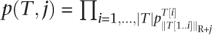is the occurrence probability of subtranscript T to occur after j letters of a read.

Lemma 2. Let e, i, q ∈ ; t ∈ ; T ∈ Δ(q). R can be calculated using the following recurrence:

with

and

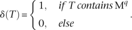Proof. See below.

Accordingly, the sensitivities S(n, e, t) for all e = 0, … , k and t = 1, … , t_max can be determined in (nkt_max4^q+k).

Extension to gapped shapes

Although “don't care” positions of gapped shapes are not immune to indels, we extend the edit distance sensitivity calculation to gapped shapes for the sake of completeness. To calculate R and S for a gapped shape Q, every q in equation 4 and Lemma 2 must be replaced by span(Q).

Algorithm 1 can be used to detect whether a common Q-gram is retained or destroyed by a transcript affecting span(Q) read characters.

Proofs

Proof of Lemma 1. Let (i, e, t, T₂) ⊆ Δⁱ, Δ = {M,R} be the set of Hamming transcripts with e errors, so that for every T₁ ∈ (i, e, t, T₂) T₁T₂ contains at least t substrings M^q. For i < 0, e < 0, or t < 0, we define (i, e, t, T₂) = Ø.

Randomly choose i, e, t ∈ , i > 0, T₂ ∈ Δ^q, and T₁ ∈ (i, e, t, T₂) and let for appropriate 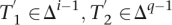, and x, y ∈ Δ. As T₁T₂ = contains at least t substrings M^q it follows that contains at least . Additionally, it holds that and thus, , and , if x = R. Because shift(x, T₂) = it follows , shift(M,T₂)) or , shift(R,T₂)) and thus:

Now, randomly choose i′, e′, t′ ∈ , x ∈ Δ, T₂ ∈ Δ^q, and ∈ (i′, e′, t′, shift(x, T₂)). It holds , and if shift(x,T₂) = T₂[1..|T₂| − 1] contains at least t′ substrings M^q, then T₂ contains at least t′ + δ(T₂). Therefore, it follows that x ∈ (i′ + 1,e′ + ||x||_E,t′ + δ(T₂), T₂) and thus:

By the definition of R it holds that R(i, e, t, T₂) = . Applied to Equations 7 and 8, Equation 3 follows.

T₂ contains exactly δ(T₂) substrings M^q, therefore (0, e, t, T₂) = {ε} if e = 0 and 0 ≤ t ≤ δ(T₂), otherwise (0, e, t, T₂) = Ø. With p(ε) = 1, Equation 2 follows.

Proof of Lemma 2. This lemma can be proven analogously to Lemma 1. Let Δ = {M, R, D, I} and (i, e, t, T₂) ⊆ Δ(i) be the set of transcripts with e errors, so that for every T₁ ∈ (i, e, t, T₂), T₁T₂ contains at least t substrings M^q.

Randomly choose i, e, t ∈ , i > 0, T₂ ∈ Δ(q), T₂ [|T₂|] ≠ I, and T₁ ∈ (i, e, t, T₂). Let for appropriate and x,y ∈ Δ. It holds that . Additionally, and thus also contain at least substrings M^q. This proves the “⊆” part of Equation 6. We omit the analog rest of the proof due to space limitations.

References

- Barski A, Cuddapah S, Cui K, Roh T, Schones D, Wang Z, Wei G, Chepelev I, Zhao K. High-resolution profiling of histone methylations in the human genome. Cell. 2007;129:823–837. doi: 10.1016/j.cell.2007.05.009. [DOI] [PubMed] [Google Scholar]
- Bentley DR, Balasubramanian S, Swerdlow HP, Smith GP, Milton J, Brown CG, Hall KP, Evers DJ, Barnes CL, Bignell HR, et al. Accurate whole human genome sequencing using reversible terminator chemistry. Nature. 2008;456:53–59. doi: 10.1038/nature07517. [DOI] [PMC free article] [PubMed] [Google Scholar]
- Burkhardt S, Kärkkäinen J. Better filtering with gapped q-grams. Fundam Inf. 2002;56:51–70. [Google Scholar]
- Burkhardt S, Crauser A, Ferragina P, Lenhof H-P, Rivals E, Vingron M. ACM; New York: 1999. q-Gram based database searching using a suffix array (Quasar). In RECOMB'99, Lyon, France; pp. 77–83. [Google Scholar]
- Chen W, Kalscheuer V, Tzschach A, Menzel C, Ullmann R, Schulz MH, Erdogan F, Li N, Kijas Z, Arkesteijn G, et al. Mapping translocation breakpoints by next-generation sequencing. Genome Res. 2008;18:1143–1149. doi: 10.1101/gr.076166.108. [DOI] [PMC free article] [PubMed] [Google Scholar]
- Dohm JC, Lottaz C, Borodina T, Himmelbauer H. Substantial biases in ultra-short read data sets from high-throughput DNA sequencing. Nucleic Acids Res. 2008;36:e105. doi: 10.1093/nar/gkn425. [DOI] [PMC free article] [PubMed] [Google Scholar]
- Döring A, Weese D, Rausch T, Reinert K. SeqAn an efficient, generic C++ library for sequence analysis. BMC Bioinformatics. 2008;9:11. doi: 10.1186/1471-2105-9-11. [DOI] [PMC free article] [PubMed] [Google Scholar]
- Herms I, Rahmann S. Computing alignment seed sensitivity with probabilistic arithmetic automata. Lect Notes Comput Sci. 2008;5251:318–329. [Google Scholar]
- Hillier LW, Marth GT, Quinlan AR, Dooling D, Fewell G, Barnett D, Fox P, Glasscock JI, Hickenbotham M, Huang W, et al. Whole-genome sequencing and variant discovery in C. elegans. Nat Methods. 2008;5:183–188. doi: 10.1038/nmeth.1179. [DOI] [PubMed] [Google Scholar]
- Huson DH, Auch AF, Qi J, Schuster SC. Megan analysis of metagenomic data. Genome Res. 2007;17:377–386. doi: 10.1101/gr.5969107. [DOI] [PMC free article] [PubMed] [Google Scholar]
- Jiang H, Wong WH. SeqMap: Mapping massive amount of oligonucleotides to the genome. Bioinformatics. 2008;24:2395–2396. doi: 10.1093/bioinformatics/btn429. [DOI] [PMC free article] [PubMed] [Google Scholar]
- Jokinen P, Ukkonen E. Two algorithms for approximate string matching in static texts. Lect Notes Comput Sci. 1991;520:240–248. [Google Scholar]
- Kent W. BLAT—the BLAST-like alignment tool. Genome Res. 2002;12:656–664. doi: 10.1101/gr.229202. [DOI] [PMC free article] [PubMed] [Google Scholar]
- Langmead B, Trapnell C, Pop M, Salzberg S. Ultrafast and memory-efficient alignment of short DNA sequences to the human genome. Genome Biol. 2009;10:R25. doi: 10.1186/gb-2009-10-3-r25. [DOI] [PMC free article] [PubMed] [Google Scholar]
- Levenshtein VI. Binary codes capable of correcting deletions, insertions and reversals. Sov Phys Dokl. 1966;10:707. [Google Scholar]
- Ley T, Mardis E, Ding L, Fulton B, McLellan M, Chen K, Dooling D, Dunford-Shore B, McGrath S, Hickenbotham M, et al. DNA sequencing of a cytogenetically normal acute myeloid leukaemia genome. Nature. 2008;456:66–72. doi: 10.1038/nature07485. [DOI] [PMC free article] [PubMed] [Google Scholar]
- Li M, Ma B, Kisman D, Tromp J. PatternHunter II: Highly sensitive and fast homology search. Genome Inform. 2003;14:164–175. [PubMed] [Google Scholar]
- Li H, Ruan J, Durbin R. Mapping short DNA sequencing reads and calling variants using mapping quality scores. Genome Res. 2008;18:1851–1858. doi: 10.1101/gr.078212.108. [DOI] [PMC free article] [PubMed] [Google Scholar]
- Li R, Li Y, Kristiansen K, Wang J. SOAP: Short oligonucleotide alignment program. Bioinformatics. 2008;24:713–714. doi: 10.1093/bioinformatics/btn025. [DOI] [PubMed] [Google Scholar]
- Lin H, Zhang Z, Zhang MQ, Ma B, Li M. Zoom! Zillions of oligos mapped. Bioinformatics. 2008;24:2431–2437. doi: 10.1093/bioinformatics/btn416. [DOI] [PMC free article] [PubMed] [Google Scholar]
- Ma B, Tromp J, Li M. PatternHunter: Faster and more sensitive homology search. Bioinformatics. 2002;18:440–445. doi: 10.1093/bioinformatics/18.3.440. [DOI] [PubMed] [Google Scholar]
- Morin RD, O'Connor MD, Griffith M, Kuchenbauer F, Delaney A, Prabhu A-L, Zhao Y, McDonald H, Zeng T, Hirst M, et al. Application of massively parallel sequencing to microrna profiling and discovery in human embryonic stem cells. Genome Res. 2008;18:610–621. doi: 10.1101/gr.7179508. [DOI] [PMC free article] [PubMed] [Google Scholar]
- Myers EW. A fast bit-vector algorithm for approximate string matching based on dynamic programming. JACM. 1999;46:395–415. [Google Scholar]
- Navarro G, Raffinot M. Cambridge University Press; Cambridge, MA: 2002. Flexible pattern matching in strings, Ch. 6.5; pp. 162–166. [Google Scholar]
- Owolabi O, McGregor DR. Fast approximate string matching. Softw Pract Exper. 1988;18:387–393. [Google Scholar]
- Rasmussen K, Stoye J, Myers G. Efficient q-gram filters for finding all ε-matches over a given length. J Comput Biol. 2006;13:296–308. doi: 10.1089/cmb.2006.13.296. [DOI] [PubMed] [Google Scholar]
- Rumble S, Brudno M. SHRiMP—SHort Read Mapping Package. 2008. http://compbio.cs.toronto.edu/shrimp.
- Smith TF, Waterman MS. Identification of common molecular subsequences. J Mol Biol. 1981;147:195–197. doi: 10.1016/0022-2836(81)90087-5. [DOI] [PubMed] [Google Scholar]
- Wang J, Wang W, Li R, Li Y, Tian G, Goodman L, Fan W, Zhang J, Li J, Zhang J, et al. The iploid genome sequence of an Asian individual. Nature. 2008;456:60–65. doi: 10.1038/nature07484. [DOI] [PMC free article] [PubMed] [Google Scholar]