

Abstract
Motivation: Modern HIV-1, hepatitis B virus and hepatitis C virus antiviral therapies have been successful at keeping viruses suppressed for prolonged periods of time, but therapy failures attributable to the emergence of drug resistant mutations continue to be a distressing reminder that no therapy can fully eradicate these viruses from their host organisms. To better understand the emergence of drug resistance, we combined phylogenetic and statistical models of viral evolution in a 2-phase computational approach that reconstructs mutational pathways of drug resistance.
Results: The first phase of the algorithm involved the modeling of the evolution of the virus within the human host environment. The inclusion of longitudinal clonal sequence data was a key aspect of the model due to the progressive fashion in which multiple mutations become linked in the same genome creating drug resistant genotypes. The second phase involved the development of a Markov model to calculate the transition probabilities between the different genotypes. The proposed method was applied to data from an HIV-1 Efavirenz clinical trial study. The obtained model revealed the direction of evolution over time with greater detail than previous models. Our results show that the mutational pathways facilitate the identification of fast versus slow evolutionary pathways to drug resistance.
Availability: Source code for the algorithm is publicly available at http://biorg.cis.fiu.edu/vPhyloMM/
Contact: pbuendia@miami.edu
1 INTRODUCTION
The incidence of disease and death from viral infections with HIV-1, hepatitis B virus (HBV) and hepatitis C virus (HCV) has been dramatically reduced with the advent of modern combination therapies. In patients on modern HIV-1 antiretroviral therapy, viral levels are suppressed to almost undetectable levels ( <50 copies/ml), but HIV is known to persist in latent reservoirs in resting CD4+ T cells and also as free virus in the plasma. Drug-resistant strains have emerged in patients with sub-optimal therapies or with lax adherence to a treatment regime (Bailey et al., 2006; Bangsberg, 2008; Bangsberg et al., 2004; Kolber, 2007; Palmer et al., 2008; Sethi et al., 2003).
Advances in the area of computer science and information technology facilitate the study of viral evolution and aid in the development of new therapy design systems. Genotype-based prediction systems of drug-resistance, for example, represent a new frontier in the fight against the emergence of drug-resistant strains. A majority of these systems, however, only predict the current phenotype and do not predict future drug resistance (De Luca et al., 2003; HIVdb, 2002; Lengauer and Sing, 2006; Mazzotta et al., 2002; Savenkov et al., 2005; Shafer and Schapiro, 2005). Other models that seek to describe viral evolution fail to include a phylogenetic context of ‘within-host’ population dynamics. These models do not utilize the nucleotide information content in viral sequences and often do not consider the sampling time or host origin (Beerenwinkel et al., 2004, 2005a, 2005b; Foulkes and De Gruttola, 2003; Pan et al., 2007).
Single-genome viral RNA sequences, representative of both majority and minority viral populations within a patient, are an ideal source of molecular information in the study of in vivo viral evolution. Multiple studies demonstrate the significance of these clonal sequences in the framework of longitudinal studies for the understanding of the disease progression in a patient (Bailey et al., 2006; Delobel et al., 2005; Kieffer et al., 2004; Mens et al., 2007; Resch et al., 2005). Pyrosequencing has emerged as a cost-effective sequencing methodology that is based on the detection of released pyrophosphate during DNA synthesis (Ronaghi, 2001). This technology has led to the identification of previously undetectable drug resistant HIV variants from drug-naïve patients at the start of therapy (Simen et al., 2007). With the arrival of the 454 pyrosequencing technology, the availability of in vivo information of the minority and majority HIV species within a patient and their corresponding frequencies will result in the development of new statistical and phylogenetic models such as the one proposed here that aim to estimate the direction of the virus evolution in response to treatment.
Several methods that estimate the phylogenetic relationship of within-patient serially sampled sequence data have been published since 2000 (Buendia and Narasimhan, 2004, 2007; Drummond and Rambaut, 2003; Drummond and Rodrigo, 2000; Rambaut, 2000; Ren et al., 2001). The performance of the different methods was compared in two earlier studies, suggesting that MinPD, a method used in our current research, had a better overall performance (Buendia and Narasimhan, 2008; Buendia et al., 2006). HIV evolution within a patient exhibits strong evidence of continual positive selection, reflecting the successive fixation of advantageous mutations and the extinction of unfavorable lineages (Rambaut et al., 2004). Under continuous drug pressure, HIV resistance mutations tend to accumulate along certain pronounced ‘mutational pathways’, leading to groups of positively associated mutations (Moya et al., 2000; Shafer and Schapiro, 2005). It has been shown, for example, that for patients on Efavirenz therapy, mutation 101E most often appears after the appearance of mutation 190S in the same genome (Beerenwinkel and Drton, 2007). Understanding the series of mutational pathways serves as a starting point for the planning of long-term antiviral treatments that seek to prevent future drug failures.
Mutagenetic tree models (Fig. 5) have been used to model the stochastic accumulation of mutations and are based on strong statistical concepts but are restrictive in their assumptions as discussed below (Beerenwinkel et al., 2005a). Another limitation of the model is the failure to include a phylogenetic context of ‘within-host’ population dynamics. Phylogenetics is the study of the evolutionary ancestor/descendant relationships between species and has been critical for understanding the biology and evolution of HIV (Hillis, 1999). A modification of the mutagenetic tree model that incorporates phylogenetic analysis was proposed later but did neither consider nucleotide data, revertant mutations, sampling time nor patient origin (Beerenwinkel and Drton, 2007).
Fig. 5.

Mtreemix mutagenetic tree for Efavirenz.
The advantage of our proposed method is that it combines statistical and phylogenetic models of evolution and takes into account the complete information available in viral RNA/DNA clonal nucleotide sequences sampled serially from the same hosts. The new method is built upon the features of Sliding MinPD, an enhanced version of MinPD that models the evolution of the virus in its host environment through serial evolutionary trees and networks (Buendia and Narasimhan, 2004, 2007). In a second step, the evolutionary trees are reduced to a transitional Markov model by translating the nucleotide sequences into drug resistance genotypes and computing the transition probabilities between those genotypes as described in a related study (Foulkes and De Gruttola, 2003).
2 METHODS
We propose a new algorithm, ‘vPhyloMM’, which uses phylogenetic and Markov model approaches to model the evolution of viral drug resistance. ‘vPhyloMM’ characterizes the transition from sensitive to resistant virus and from one category of resistance to another by inferring distinct mutational pathways with corresponding transition rates and linkage relationships. The 2-step approach to reconstructing the mutational pathways of drug-resistance is to infer the within-host evolutionary relationships and subsequently construct a Markov model from the evolutionary relationships (Fig. 3).
Fig. 3.

Flowchart of the reconstruction of mutational pathways. Label pp indicates per patient results.
2.1 Phase 1: phylogenetic model
The phylogenetic analysis was performed with ‘Sliding MinPD’, a distance-based program that infers evolutionary lineages from within-host longitudinal clonal sequences without assuming a molecular clock (Buendia and Narasimhan, 2004, 2007). The program searches for the closest ancestor of each sequence among all previous sampling times. The phylogenetic model used in the current study does not assume recombination events in the evolutionary history of the sequences. Detectable recombination events are rare in drug suppressed virus as cell co-infection is rare and the residual viremia is dominated by a homogeneous population of viruses (Bailey et al., 2006; Fraser, 2005; Levy et al., 2004). The recombination detection feature was therefore turned off to focus on tree-like evolutionary relationships. There are no other limiting assumptions in the phylogenetic model. A serial evolutionary tree is constructed from the patient's viral sequences for each patient separately using the program Sliding MinPD (Fig. 1). Sliding MinPD calculates the statistical significance for all predictions in terms of bootstrap values and presents the results in a serial evolutionary tree. The bootstrap support is calculated for each ancestor/descendant relationship and placed after the descendant sequence in the tree visualization (Fig. 1). The ancestor/descendant transitions described in the trees are used to compute the transition frequencies between genotypes.
Fig. 1.

Representation of the within-patient evolutionary relationships of the virus for each patient. The tree for patient 5 from the Bacheler et al. (2000) dataset is shown with bootstrap support values enclosed in square brackets, and solid horizontal lines indicating genetic distance.
The drug resistant genotype for each viral sequence was determined by looking at the codon to amino acid translation as shown in an example in Figure 2. Each genotype was described by a binary sequence of 0's and 1's. A 1 indicates that the amino acid is present at that position, a 0 that it is not. For example, a 1 was added if the codon AAT or AAC appeared in amino acid position 103 of the reverse transcriptase (RT) gene indicating the presence of Asparagine (N). We reference a particular nucleotide sequence by either its binary sequence or a position code that uses the mutation position numbers. Figure 2 shows the binary codes for seven positions of interest. The markers used in the example are: 0 = wildtype, 1 = 100I, 2 = 101E, 3 = 101Q, 4 = 103N, 5 = 108I, 6 = 190S, 7 = 225H. For a nucleotide sequence containing 103N and 225H and otherwise wild-type amino acids, we have the binary sequence 0001001 or the position code 47 (drug resistant amino acids at positions 4 and 7 are present).
Fig. 2.

Binary sequences describing the viral genotype for seven markers.
2.1.1 Genotype clustering techniques
Two types of genotype clustering techniques were introduced at different steps during the processing of the data:
Ancestral sequences that share the same genotype and a small genetic distance from a descendant were grouped together to compute the bootstrap support at the genotype level instead of the nucleotide level.
Descendant sequences that share the same genotype and are linked to the same ancestor for the same two time points were counted as a single transition.
The genotype clustering feature for the computation of the bootstrap support, case (a) above, was introduced into Sliding MinPD to obtain a more accurate support for the ancestor/descendant predictions when the focus is on transitions between genotypes. It is known that the sensitivity of phylogenetic predictions is negatively affected when there are highly homologous sequences in the dataset, which is the case when some of the viral sequences had insufficient time to evolve between sampling times. Choosing a smaller but representative set of divergent sequences often provides the same phylogenetic tree far more efficiently (Rosenberg and Kumar, 2001). The approach implemented in Sliding MinPD does not remove sequences, but instead clusters ancestral sequences with respect to their similarity (distance clustering) and identical genotype for the computation of the bootstrap support per cluster. In the evolutionary tree, each cluster is represented by the ancestor sequence with minimum genetic distance to the descendant sequence.
The second clustering method, case (b) above, serves to remove sampling bias. Many similar sequences may be sampled at a given time point representing the same ‘predominant’ quasispecies. The evolution from the ancestor virus to this swarm of virus should count as one transition if they all share the same common ancestor and the same genotype. This approach aggregates all such transitions within a patient to compute the transition frequencies among genotypes from the ancestor/descendant relationships.
2.1.2 Codon frequencies
Once the ancestor/descendant predictions for single clonal sequences have been generated, it is possible to also calculate the codon transition frequencies for each of the positions associated with drug resistance. These statistics provide an additional layer of prediction support for the design of the model. For transitions from an ancestral genotype, the ancestral codon at a particular amino acid position may be indicative of a preference for a particular mutational pathway. This information expands the Markov model prediction capability.
Let N = nij be the observed number of transitions i → j between an ancestral genotype i to a descendant genotype j over all time intervals for two genotypes i, j ∈ G. Let c(i → j)k,p ∈ {0, 1} be the indicator of the presence of a three-letter codon c over the alphabet Σc ∈ {A, C, G, T} at position pin an ancestral clone involved in a transition k from i to j. Each position represents a particular position along the DNA sequence that is associated with drug resistance. The frequency of a particular ancestral codon c at position p for transitions i → j is calculated by
Fisher exact tests were carried out to calculate the significant association between codons and transitions departing from a particular ancestral genotype. The Benjamini and Hochberg (1995) correction for multiple comparisons was used when more than two tests were carried out for an ancestral genotype
2.2 Phase 2: Markov model
For the second phase of the vPhyloMM algorithm, the evolutionary trees of all patients were reduced to a compact set of transitions and the transition counts between ancestor/descendant genotypes were computed as previously described. The genotypes are associated with the amino acid mutations that impart resistance to a particular drug (Fig. 2). Only the transitions with non-parametric bootstrap support >0.7 were chosen to determine the topology of the Markov model.
A Markov process is a probabilistic model describing the progression of a system through a sequence of states. The genotypes used in this analysis represent the states in the Markov model and can be thought of as arising from a continuous time Markov process as the sampling times vary among patients. A continuous time discrete-state stochastic process is called a Markov chain if for times t<s, where Z(s) and Z(t) are the states at times s and t respectively and pij(t, s) is the probability of transitioning from state i to j from time t to time s, the conditional probability mass function satisfies the following Markov properties.
pij(t, s) = P[Z(s) = j|Z(t) = i], i.e. the probability of moving from state i to state j is only dependant on the immediate previous state.
P(t, s) = P(s − t), i.e. the probability of moving between time points t and s is only dependant on the time elapsed, s − t, not the absolute time.
The variables used in the model are obtained from the results of the phase one phylogenetic analysis. Time t and s are the observed sampling times for an inferred ancestor/descendant transition. States i and j represent the ancestor and descendant genotypes. The number of transitions from i to j were aggregated for all such ancestor/descendant relationships among all trees and are represented by N(i, j). Albert (1962) presented parameter estimates for a continuous time Markov process that are analogous to estimates for a discrete time Markov chain (Albert, 1962). Let P(t) be the transition probability matrix for a continuous Markov model. In a time interval t, the system undergoes a change of state (or stays in the same state, a repetition) according to a set of probabilities associated with the state. P(t) can be expressed in the form
where Q is the infinitesimal generator of the continuous Markov process. Q is a m × m matrix encoding the time independent transition rates for a set of m states. As shown by Albert (1962), Q can be estimated by
with N(i, j) the number of transitions from states i to j, and AT(i) the total time i is occupied over all P patients (Albert, 1962). A Markov model was used in an earlier study to determine whether the presence of certain mutations among drug-sensitive viruses elevates the risk of developing high-level drug resistance (Foulkes and De Gruttola, 2003). A similar model was implemented in our current study to model viral evolution as a system that can be in one of a set of k distinct genotype states and transitions between the states in discrete time intervals. The difference between the two models is that the genotypes and transitions between genotypes are computed based on the phylogenetic relationship of the sequences, while in the above cited study a K-means clustering method was used instead.
The transition model for one time interval can be represented as a directed graph with the P(t) probabilities used as the edge weights (Fig. 4). Dijkstra's shortest path algorithm was adapted to find the most probable path between a start and a destination state by taking the log of the probabilities. For comparison between competing models, however, we calculated the all pairs most probable paths and focused on the most probable paths with up to k edges. All possible paths of length k were found using matrix multiplication and then sorted first by source and then by weight. Cyclic paths were identified as those having duplicate vertices and were not considered for output.
Fig. 4.

Mutational pathways for Efavirenz. Transitions that appear in the competing MTreemix model are highlighted by bold lines.
Low support states were pruned from the model if they were connected through edges with transition counts ≤x, with x the pruning threshold. In cases when there is a particular start state in the model, such as the ‘wild type’ genotype in the example used below, ancestorless states are reconnected to the start state by computing the transitive closure and all pairs' shortest paths for the non-pruned graph using an implementation of the Floyd–Warshall algorithm.
2.2.1 Implementation
The add-in R library ‘msm’ developed by Christopher Jackson (http://cran.r-project.org/web/packages/msm/index.html) was used to calculate the transition probabilities of the Markov model. Perl scripts were developed to format input and output data, to run Sliding MinPD and the R scripts, to compute the statistics and evaluate the model.
2.3 Empirical data
The data used to build the model consists of sequenced clones of length 984 bp from the HIV-1 pol gene, collected from 120 patients at different time points during phase II clinical studies of the RT inhibitor ‘Efavirenz’. (Bacheler et al., 2000). Patients participating in those studies received combination therapies that also included AZT, 3TC and Indinavir. Seven amino acid mutations that are associated with drug resistance to Efavirenz were studied: L100I, K101E, K101Q, K103N, V108I, G190S and P225H.
3 RESULTS
A Markov state transition model was used to represent the mutational pathways of drug-resistance. For states described by a binary sequence of seven possible mutations, which have been observed for Efavirenz, there are 27 = 128 possible states; however, only a few states are represented in the data, resulting in a probability transition matrix of smaller dimension. Twenty-six genotypes were observed among all patients with a maximum of three mutations linked on the same viral genome. Low support states, those connected to transitions that were only observed once, were pruned from the model, reducing the model to 12 genotype states. The 16-week probability of transitioning from one state to another or staying in the same state was computed for the model shown in Figure 4. Only observed transitions are represented in the directed graph. The probability of transitioning in a different time frame can also be computed using the formulas presented in the Section 2.
3.1 Model comparison and statistics
A competing model, called the mutagenetic tree model, which can be generated from binary sequences using the programs Mtreemix or RTreemix (Beerenwinkel et al., 2005a), is shown in Figure 5. The mutagenetic tree model is built on sound statistical theory, but is restrictive in its assumptions and does not consider mutations that revert to a previous state. Nucleotide data are not used. Neither patient origin nor the time when a viral sequence was sampled is considered. Each node represents only the transition from wildtype to drug resistance for one specific amino acid position, while the nodes in our Markov model represent the linked mutation genotype, leading to a more informative model.
When the binary sequences are obtained from clonal sequences instead of consensus sequences, the mutagenetic tree is comparable to the mutational pathways obtained by our method. The two methods, however, do not display equivalent information. The comparison focuses, therefore, on the shared states and transitions between the two models. The edges in the mutagenetic tree are weighted with the conditional probability of the child event given that the parent event has occurred and are not based on time. The mutagenetic tree has fewer states as it represents a cumulative process; once a mutation is added it is not lost and transitions between disjoint genotypes (that do not share the same mutations) are not possible. Both models share a similar topology for the most probable paths, but due to the exhaustive scope of our approach, we are able to capture additional details that reveal novel evolutionary patterns of drug resistance.
As seen in the model in Figure 4, the probability of remaining in the same state (a repetition) after 16 weeks is always larger than the probability of transitioning to a different state. The repetition probability for the wild state decreases from 0.972 for the 1-week interval, to 0.648 for the 16-week interval and to 0.258 for the 52-week interval. The most probable transition from the wild-type state is to genotype state 103N with probability 0.2476. It is interesting to note that 103N incoming transitions have higher probability than outgoing transitions, with the exception of transitions to and from genotype 103N/225H (0.115 and 0.099, respectively). Once the virus acquires the 103N/225H genotype the model predicts that it will maintain this genotype for a prolonged period of time or add mutations to it (since the state has other outgoing transitions). The reverse can be observed for viruses with the 103N mutations linked with a non-225H mutation on the same genome, in which case the viruses have a higher probability of losing the non-225H mutation in the same period of time. It should be noted that this conclusion cannot be drawn from the mutagenetic model in Figure 5 as reversions are not considered. While reversions are rare and it is possible that inferred reversions are a consequence of fluctuations in virus sub-populations rather than actual mutations, this possibility is allowed by our model, as both processes can lead to previously observed genotypes.
A separate path that does not involve 103N and goes from wildtype to 190S to 101E/190S (0→6→26 using the position codes) was observed in both models. As can be observed from Figures 4 and 5, among the five transitions with highest probability are two that appear in both models: transitions from wildtype to 103N, and from 190S to 101E/109S. Table 1 shows the 10 most probable paths that start at the wildtype state with up to four states. It is interesting to note that a few of these paths also appear in the mutagenetic model, such as 0→4→47, 0→4→45, 0→4→34 (the numbers in parentheses indicate the position code of the mutation). In our model, we also observe transitions from wildtype to a genotype state with two mutations, for example, to 103N/225H (47). It should be mentioned that the probability of this single transition is very low (0.033) and that a separate path through 103N(4) exists with high single transition probabilities, suggesting that the transitions occur so quickly that the intermediate state (with only 103N) will not be observed.
Table 1.
Ten highest 16-week transition probability paths from wildtype
| Probability | Ancestor | Descendant | States | s1 | s2 | s3 | Total |
|---|---|---|---|---|---|---|---|
| 0.2467 | 0 | 4 | 2 | 0 | 4 | 129 | |
| 0.0330 | 0 | 47 | 2 | 0 | 47 | 7 | |
| 0.0320 | 0 | 45 | 2 | 0 | 45 | 10 | |
| 0.0283 | 0 | 47 | 3 | 0 | 4 | 47 | 170 |
| 0.0165 | 0 | 45 | 3 | 0 | 4 | 45 | 151 |
| 0.0123 | 0 | 34 | 2 | 0 | 34 | 4 | |
| 0.0080 | 0 | 14 | 2 | 0 | 14 | 3 | |
| 0.0060 | 0 | 34 | 3 | 0 | 4 | 34 | 137 |
| 0.0050 | 0 | 457 | 3 | 0 | 4 | 457 | 134 |
| 0.0033 | 0 | 4 | 3 | 0 | 47 | 4 | 11 |
Column ‘Total’ indicates the number of observed transitions between the two states. Position codes: 0 = wildtype, 1 = 100I, 2 = 101E, 3 = 101Q, 4 = 103N, 5 = 108I, 6 = 190S, 7 = 225H. first, second and third states in path: s1, s2, s3.
The frequencies of the ancestral codon for each ancestor/descendant transition were computed as described in the methods section. In order to obtain this information, it is imperative that longitudinal clonal nucleotide sequences be used in the framework of phylogenetic analysis. Nucleotide consensus sequences (polyclonal sequences), on the other hand, merely summarize the viral population and do not identify different variants or reveal their evolutionary impact. Using the method described previously, we obtained the frequencies for wild-type transitions shown in Table 2. The most prevalent codon is shown in the column header and a dash in the rows below the header indicates that it was the only codon observed for that particular ancestor/descendant transition. The data can be used to identify codon frequency patterns that indicate a preference for one mutational path over another. For example, codon GGC at position 6 has been observed 88% of the times for transitions 0→6 from wildtype to 190S (only codon counts of 5 or more are considered); but in other paths, it has been observed at only low frequencies or not at all. In fact, the presence of codon GGC at position 6 indicates a significant preference for the 0→6 transition (P < 0.001 for a Fisher exact test with subsequent Benjamini and Hochberg correction). A few other significant codons of lesser relevance were found, such as CCC at position 7 indicating a preference for the 6→26 transition (P = 0.001), GGA at position 6 indicating a preference for the 2→0 reversion (P = 0.002) and AAC at position 4 indicating a preference for the 14→4 reversion (P = 0.001). This information is useful when developing a prediction system in combination with the multinomial probability distribution for transitions from a given state in the Markov model.
Table 2.
Frequency of observed synonymous codons for transitions from wildtype
| Ancestor | Descendant | pos:1 (TTA) | pos: 2; 3 (AAA) | pos: 4 (AAA) | pos: 5 (GTA) | pos: 6 (GGA) | pos: 7 (CCT) |
|---|---|---|---|---|---|---|---|
| 0 | 0 | CTA (3%) | AAG (1%) | AAG (3%) | GTG (8%); GTC (1%) | GGC (5%); GGG (2%); GCA (1%) | CCC (10%); CTT (1%) |
| 0 | 6 | – | – | AAG (5%) | – | GGC (88%)a | CCC (28%) |
| 0 | 4 | CTA (6%); TTG (3%) | AGA (2%)a; AAG (1%) | AAG (3%); AGA (1%) | GTG (6%); GTT (1%); GTC (1%) | GGG (4%); GGC (2%) | CCC (10%); CCG (3%)a |
| 0 | 47 | – | – | AGA (3%) | – | GGC (3%) | – |
| 0 | 45 | TTG (2%) | – | – | – | GGC (40%); GGG (4%) | – |
| 0 | 34 | – | – | AAG (31%) | – | – | CCC (23%) |
| 0 | 2 | – | – | AGA (29%) | – | GGC (10%) | CCC (19%) |
| 0 | 24 | – | – | – | – | – | – |
| 0 | 14 | – | – | – | – | GGC (57%) | CCC (29%) |
Most prevalent codon appears in parentheses in header line; transitions with this codon are identified by a dash. Position codes are as before.
asignificant preference for the indicated transition.
3.2 Model validation
In order to test whether the virus evolution is independent from the host environment and independent of the time of sampling, we ran several correlation tests involving the variable of interest, number of transitions. A transition in our model is defined as a change in one or more of the six amino acid positions, giving equal weight to a transition with 1, 2 or more amino acid changes. Statistical analysis found no significant correlation between number of transitions and sampling time within a patient, suggesting independence of time and transition count. Moreover, when looking at parameters that co-vary between patients, significant correlations were found between number of sampling times and number of transitions, (r = 0.513, P = 0.04), and number of sequences per sampling point and number of transitions (r = 0.45, P = 0.013), indicating that the transition counts are affected by the number of sampling points and number of sequences sampled, two variables which are independent of the host environment.
In addition, the method by DeGruttola and Foulkes (2004) was used to test formally that the first-order, stationary Markov model holds for all transition and all time points (De Gruttola and Foulkes, 2004). The test is based on simulated datasets generated from the estimated Markov model and is used to assess whether the Markov properties (presented above) hold. The simulation test is performed using the following algorithm.
Compute eijl, the expected transition frequencies between genotypes i and j (binary sequences) in time interval l, by using the Markov transition matrix pij for interval l and the following formula: eijl = ni.lpijl, with ni.l the observed number of all transitions from i in interval l.
Based on ni.l, we obtain n′ijl, the simulated observed number of transitions by drawing ni.l times from a multinomial distribution for interval l with probabilities pi1l, pi2l,…, pikl with k the number of genotypes/states.
Repeat step 2, B = 100 times to obtain 100 n′ijl for each i, j, l.
Calculate
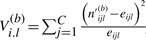 for b = 1,…, B with C the number of states. Order the V(b)i.l, such that the largest V value is in V(b)(CxM).
Calculate the r-th expected order statistic
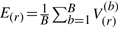 for r = 1,…, C × M. E(r) is the mean V value among all 100 simulations for a given r.
Let D(r)(b) =|V(r)(b) − E(r)| (the difference from the mean for each simulation) and record the 95% confidence interval (CI) of the distribution of D(r)(b) over all b = 1,…, B.
Calculate the r-th order statistics D(r) = |V(r) − E(r)| with V(r) similar to the V from equation in (4), but with nijl instead of n′ijl.
Significance is assessed by comparing the D(r) to the 95% CI of the distribution of D(r)(b) over all b = 1,…, B.
Figure 6 shows the result of the validation process, which compares the order statistics of V to their expected values. Each circle represents a particular time interval and a start state. We restricted our application to the six most frequently observed time intervals to reduce the sparseness of data, but included all 12 states from the model shown in Figure 4. Thus, a total of 6 × 12 = 72 dots are plotted. The lines in the figures correspond to the 95% confidence bands for the 72nd (dashed) and 71st (dotted) order statistics. A single dot outside the dashed lines or two dots outside the dotted lines suggest a departure from the Markov assumption. Using this approach, it can be noted that the number of observed transitions is slightly greater than expected; however, this difference is not significant. One point, in particular, has a marked distance from the other points (4 weeks, wild-type state), but the outlier is well within the 95th percentile (dashed line).
Fig. 6.

Observed versus expected statistics.
The empirical data used in the model creation was analyzed for putative recombination events. The few predicted recombination events were not found to affect the model. These events were among the same genotype or had low bootstrap support leading to their automatic exclusion from the model.
4 DISCUSSION
A 2-step algorithm that combines phylogenetic analysis and a Markov process was developed to capture the mutational pathways of drug resistance, i.e. branching structures in which the evolution of specific mutations can be traced along directed paths. Serially sampled nucleotide sequences from HIV-1 viruses were studied using a per-patient phylogenetic approach to model the within-host evolution of the virus via serial evolutionary trees. The Markov model step recovered a map of the potential pathways for drug-resistance for a specific drug by reducing the set of serial evolutionary trees to an n-state Markov transition model showing the transitions from one mutation state to another. Our algorithm should be applicable to fast evolving viruses that develop drug resistant mutations under drug pressure.
We showed that the most probable paths in our model are comparable to those of the mutagenetic tree model generated by MTreemix 1.3 (Beerenwinkel et al., 2005a), a program that uses an EM algorithm for model fitting from binary sequence data. While the MTreemix program can also generate a mixture model of k mutagenetic trees to overcome the limitations of a single tree that does not capture all the pathways, our model goes a step further in representing linked mutations as states and allows for mutations to revert back to a previous state. In our analysis of an HIV-1 dataset from patients on an Efavirenz therapy, we showed that although most mutations added onto a 103N genotype may revert back to wildtype, the 225H mutation linked on the same genome with the 103N mutation has a higher probability of persisting over time. The phylogenetic analysis during the first phase of our approach made it possible to calculate the frequencies of observed ancestral codons for all ancestor/descendant relationships and for the six positions associated with drug resistance. This information may complement the prediction process of the Markov model as a particular codon may be associated with a particular path.
It has been suggested that with decreasing viral load, cell co-infection falls rapidly and viral populations become more homogenous (Bailey et al., 2006; Levy et al., 2004). Recombination should therefore have little effect on the emergence of drug resistance during therapy and is difficult to detect under these conditions (Fraser, 2005). In the analyzed dataset, the inferred recombination events were few and did not affect the model. Incorporating recombination into the model would lead to a greater number of unlinked genotypes, as different parts of a gene sequence would have different ancestors. This would in turn affect the transition model, increasing the number of states and reducing the power of the model. We have assumed that mutations occur at the time they are observed. An interval censoring correction could be applied to some of the larger interval lengths; however, no qualitative and little quantitative differences were found in a related study when using the midpoint of time intervals as the time at which mutations occur (Foulkes and DeGruttola, 2003). This small bias may account for the underestimation of order statistics in Figure 6. When using the mean pairwise genetic distance (MPD) between two time points as an estimate of the evolutionary rate, we found that 65% of patients had a significant correlation (P < 0.05) between MPD and sampling time, and 88% of those patients showed their MPD to be negatively correlated with time. This observation did not, however, affect the assumptions of independence for the Markov model, as the measure of interest is the observed transitions count. A transition is defined as a change at one or more of the six amino acid positions. The transition count was found to be independent of sampling time and host environment.
The inclusion of clonal sequence data distinguishes our model from other models that make use of polyclonal sequences (obtained through bulk PCR methods), which only show the consensus genotype of the viral population at a given time point. Single-genome (clonal) viral RNA sequences, representative of both majority and minority viral populations within a patient, are an ideal source of molecular information in the study of in vivo HIV evolution. The ultra-deep 454 pyrosequencing technology generates reads of up to ∼400 bp in length, data that is ideal for use with our proposed methods as it allows the identification of linked mutations. This new technology has led to the identification of a significantly larger proportion of HIV-infected, treatment-naive persons as harboring drug-resistant viral variants (Simen et al., 2009). We incorporated clonal sequence data into our model by inferring the ancestor/descendant transitions for each patient. We also calculated the frequency of ancestral codons at drug resistant positions for all observed transitions and found that certain codons appear more frequently in certain transitions than others. While available data are insufficient to allow us to expand the number of states to include the impact of synonymous codons, future work will focus on incorporating such information as covariates into the Markov model likelihood.
Antiviral therapies against HIV-1, HBV and HCV currently in the market are successful at suppressing virus populations to undetectable levels, but they do not eliminate the virus. An increase in viral load at any time can lead to an increase in viral evolution and to drug resistant mutations leading to therapy failure. Some reasons for therapy failures are: non-optimal adherence to a therapy, limited access to therapy in non-industrialized countries, lack of optimal therapy after previously failed therapy and preexisting drug resistant mutations. With the availability of clonal (pyro-) sequences from patients at the beginning of therapy and at points of failure, the method described here will allow for the reconstruction of new pathways of drug resistance. We believe that the use of phylogenetic methods that model molecular processes in viral evolution under drug pressure and analyze the full information content in nucleotide sequence data will lead to the identification of distinct evolutionary pathways to multiple drug resistance.
Findings from the proposed research may have implications for clinicians; particularly in relationship to treatment strategies that delay, or potentially even reverse drug resistance and are applicable to HIV, HBV and HCV anti-viral therapies alike. Future plans include the development of a therapy outcome prediction system that combines the phylogenetic and statistical models presented here, information from clonal viral sequences and clinical and immune response data.
ACKNOWLEDGEMENTS
We thank Monique Courtenay for her involvement in the initial phase of this project.
Funding: University of Miami Developmental Center for AIDS Research (D-CFAR) National Institute of Health (grant 5P30AI073961-02 to P.B. and B.C., in part). Center for Computational Science at the University of Miami (P.B.).
Conflict of Interest: none declared.
REFERENCES
- Albert A. Estimating the infinitesimal generator of a continuous time, finite state markov process. Ann. Mathemat. Stat. 1962;33:727–753. [Google Scholar]
- Bacheler LT, et al. Human immunodeficiency virus type 1 mutations selected in patients failing efavirenz combination therapy. Antimicrob. Agents Chemother. 2000;44:2475–2484. doi: 10.1128/aac.44.9.2475-2484.2000. [DOI] [PMC free article] [PubMed] [Google Scholar]
- Bailey JR, et al. Residual human immunodeficiency virus type 1 viremia in some patients on antiretroviral therapy is dominated by a small number of invariant clones rarely found in circulating CD4+T cells. J. Virol. 2006;80:6441–6457. doi: 10.1128/JVI.00591-06. [DOI] [PMC free article] [PubMed] [Google Scholar]
- Bangsberg DR. A paradigm shift to prevent HIV drug resistance. PLoS Med. 2008;5:e111. doi: 10.1371/journal.pmed.0050111. [DOI] [PMC free article] [PubMed] [Google Scholar]
- Bangsberg DR, et al. Paradoxes of adherence and drug resistance to HIV antiretroviral therapy. J. Antimicrob. Chemother. 2004;53:696–699. doi: 10.1093/jac/dkh162. [DOI] [PubMed] [Google Scholar]
- Beerenwinkel N, Drton M. A mutagenetic tree hidden Markov model for longitudinal clonal HIV sequence data. Biostatistics. 2007;8:53–71. doi: 10.1093/biostatistics/kxj033. [DOI] [PubMed] [Google Scholar]
- Beerenwinkel N, et al. Learning multiple evolutionary pathways from cross-sectional data. J. Comput. Biol. 2004;12:584–598. doi: 10.1089/cmb.2005.12.584. [DOI] [PubMed] [Google Scholar]
- Beerenwinkel N, et al. Mtreemix: a software package for learning and using mixture models of mutagenetic trees. Bioinformatics. 2005a;21:2106–2107. doi: 10.1093/bioinformatics/bti274. [DOI] [PubMed] [Google Scholar]
- Beerenwinkel N, et al. Estimating HIV Evolutionary Pathways and the Genetic Barrier to Drug Resistance. J. Infect. Dis. 2005b;191:1953–1960. doi: 10.1086/430005. [DOI] [PubMed] [Google Scholar]
- Benjamini Y, Hochberg Y. Controlling the False Discovery Rate; A practical and Powerful Approach to Multiple Testing. J. Roy. Statist. Soc. Ser. B. 1995;57:289–300. [Google Scholar]
- Buendia P, Narasimhan G. MinPD: distance-based phylogenetic analysis and recombination detection of serially-sampled HIV quasispecies. Proc. IEEE Comput. Sys. Bioinform. Conf. 2004:110–119. [PMC free article] [PubMed] [Google Scholar]
- Buendia P, Narasimhan G. Sliding MinPD: building evolutionary networks of serial samples via an automated recombination detection approach. Bioinformatics. 2007;23:2993–3000. doi: 10.1093/bioinformatics/btm413. [DOI] [PMC free article] [PubMed] [Google Scholar]
- Buendia P, Narasimhan G. The role of internal node sequences and the molecular clock in the analysis of serially-sampled data. IJBRA. 2008;4:107–121. doi: 10.1504/IJBRA.2008.017167. [DOI] [PubMed] [Google Scholar]
- Buendia P, et al. Proceedings of the International Conference on Computational Science (IWBRA). Reading, UK: 2006. Reconstructing ancestor-descendant lineages from serially-sampled data: a comparison study; pp. 807–814. [Google Scholar]
- De Gruttola V, Foulkes AS. Validation and discovery in Markov models of genetics data. Stat. Appl. Genet. Mo. B. 2004;3 doi: 10.2202/1544-6115.1104. Article 38, doi: 10.2202/1544-6115.1104] [DOI] [PubMed] [Google Scholar]
- Delobel P, et al. Persistence of distinct HIV-1 populations in blood monocytes and naive and memory CD4 T cells during prolonged suppressive HAART. AIDS. 2005;19:1739–1750. doi: 10.1097/01.aids.0000183125.93958.26. [DOI] [PubMed] [Google Scholar]
- De Luca A, et al. Variable prediction of antiretroviral treatment outcome by different systems for interpreting genotypic human immunodeficiency virus type 1 drug resistance. J. Infect. Dis. 2003;187:1934–1943. doi: 10.1086/375355. [DOI] [PubMed] [Google Scholar]
- Drummond A, Rambaut A. BEAST v1.0. 2003 Available at http://beast.bio.ed.ac.uk/ (last accessed date October 2006) [Google Scholar]
- Drummond A, Rodrigo AG. Reconstructing genealogies of serial samples under the assumption of a molecular clock using serial-sample UPGMA (sUPGMA) Mol. Biol. Evol. 2000;17:1807–1815. doi: 10.1093/oxfordjournals.molbev.a026281. [DOI] [PubMed] [Google Scholar]
- Foulkes AS, De Gruttola V. Characterizing the Progression of Viral Mutations over Time. J. Am. Stat. Assoc. 2003;98:859–867. [Google Scholar]
- Fraser C. HIV recombination: what is the impact on antiretroviral therapy? J. R. Soc. Interface. 2005;2:489–503. doi: 10.1098/rsif.2005.0064. [DOI] [PMC free article] [PubMed] [Google Scholar]
- Hillis DM. Phylogentics and the study of HIV. In: Crandall KA, editor. The Evolution of HIV. Baltimore: The John Hopkins University Press; 1999. pp. 106–111. [Google Scholar]
- HIVdb Stanford HIV drug resistance database. 2002 Available at http://hivdb.stanford.edu/ (last accessed date June 2009) [Google Scholar]
- Kieffer TL, et al. Genotypic analysis of HIV-1 drug resistance at the limit of detection: virus production without evolution in treated adults with undetectable HIV loads. J. Infect. Dis. 2004;189:1452–1465. doi: 10.1086/382488. [DOI] [PubMed] [Google Scholar]
- Kolber MA. Development of drug resistance mutations in patients on highly active antiretroviral therapy: does competitive advantage drive evolution. AIDS Rev. 2007;9:68–74. [PubMed] [Google Scholar]
- Lengauer T, Sing T. Bioinformatics-assisted anti-HIV therapy. Nat. Rev. Microbiol. 2006;4:790–797. doi: 10.1038/nrmicro1477. [DOI] [PubMed] [Google Scholar]
- Levy DN, et al. Dynamics of HIV-1 recombination in its natural target cells. Proc. Natl Acad. Sci. USA. 2004;101:4204–4209. doi: 10.1073/pnas.0306764101. [DOI] [PMC free article] [PubMed] [Google Scholar]
- Mazzotta F, et al. Proceedings of the 9th Conference on Retroviruses and Opportunistic Infections. Seattle, Washington: 2002. Real vs VirtualPhenotype: 12-Month results from the GenPherex study. [Google Scholar]
- Mens H, et al. Investigating signs of recent evolution in the pool of proviral HIV type 1 DNA during years of successful HAART. AIDS Res. Hum. Retroviruses. 2007;23:107–115. doi: 10.1089/aid.2006.0089. [DOI] [PubMed] [Google Scholar]
- Moya A, et al. The evolution of RNA viruses: A population genetics view. Proc. Natl Acad. Sci. USA. 2000;97:6967–6973. doi: 10.1073/pnas.97.13.6967. [DOI] [PMC free article] [PubMed] [Google Scholar]
- Palmer S, et al. Low-level viremia persists for at least 7 years in patients on suppressive antiretroviral therapy. Proc. Natl Acad. Sci. USA. 2008;105:3879–3884. doi: 10.1073/pnas.0800050105. [DOI] [PMC free article] [PubMed] [Google Scholar]
- Pan C, et al. The HIV positive selection mutation database. Nucleic Acids Res. 2007;35:D371–D375. doi: 10.1093/nar/gkl855. [DOI] [PMC free article] [PubMed] [Google Scholar]
- Rambaut A. Estimating the rate of molecular evolution: Incorporating non-contemporaneous sequences into maximum likelihood phylogenies. Bioinformatics. 2000;16:395–399. doi: 10.1093/bioinformatics/16.4.395. [DOI] [PubMed] [Google Scholar]
- Rambaut A, et al. The causes and consequences of HIV evolution. Nat. Rev. Genet. 2004;5:52–61. doi: 10.1038/nrg1246. [DOI] [PubMed] [Google Scholar]
- Ren F, et al. A new algorithm for analysis of within-host HIV-1 evolution. Pac. Symp. Biocomput. 2001;307:595–605. doi: 10.1142/9789814447362_0057. [DOI] [PubMed] [Google Scholar]
- Resch W, et al. Evolution of human immunodeficiency virus type 1 protease genotypes and phenotypes in vivo under selective pressure of the protease inhibitor ritonavir. J. Virol. 2005;79:10638–10649. doi: 10.1128/JVI.79.16.10638-10649.2005. [DOI] [PMC free article] [PubMed] [Google Scholar]
- Ronaghi M. Pyrosequencing Sheds Light on DNA Sequencing. Genome Res. 2001;11:3–11. doi: 10.1101/gr.11.1.3. [DOI] [PubMed] [Google Scholar]
- Rosenberg MS, Kumar S. Incomplete taxon sampling is not a problem for phylogenetic inference. Proc. Natl Acad. Sci. USA. 2001;98:10751–10756. doi: 10.1073/pnas.191248498. [DOI] [PMC free article] [PubMed] [Google Scholar]
- Savenkov I, et al. HAART outcome prediction using statistical learning methods. Antiviral Ther. 2005;10:S60. [Google Scholar]
- Sethi AK, et al. Association between adherence to antiretroviral therapy and human immunodeficiency virus drug resistance. Clin. Infect. Dis. 2003;37:1112–1118. doi: 10.1086/378301. [DOI] [PubMed] [Google Scholar]
- Shafer RW, Schapiro JM. Drug resistance and antiretroviral drug development. J. Antimicrob. Chemother. 2005;55:817–820. [Google Scholar]
- Simen BB, et al. Proceedings of the XVI International HIV Drug Resistance Workshop. Barbados: 2007. Prevalence of low abundance drug resistant variants by ultra-deep sequencing in chronically HIV-infected antiretroviral (ARV) naive patients and the impact on virologic outcomes. [Google Scholar]
- Simen BB, et al. Low-abundance drug-resistant viral variants in chronically HIV-infected, antiretroviral treatment-naive patients significantly impact treatment outcomes. J. Infect. Dis. 2009;199:693–701. doi: 10.1086/596736. [DOI] [PubMed] [Google Scholar]