Laplace-Beltrami Eigenvalues and Topological Features of Eigenfunctions for Statistical Shape Analysis

Abstract

This paper proposes the use of the surface based Laplace-Beltrami and the volumetric Laplace eigenvalues and -functions as shape descriptors for the comparison and analysis of shapes. These spectral measures are isometry invariant and therefore allow for shape comparisons with minimal shape pre-processing. In particular, no registration, mapping, or remeshing is necessary. The discriminatory power of the 2D surface and 3D solid methods is demonstrated on a population of female caudate nuclei (a subcortical gray matter structure of the brain, involved in memory function, emotion processing, and learning) of normal control subjects and of subjects with schizotypal personality disorder. The behavior and properties of the Laplace-Beltrami eigenvalues and -functions are discussed extensively for both the Dirichlet and Neumann boundary condition showing advantages of the Neumann vs. the Dirichlet spectra in 3D. Furthermore, topological analyses employing the Morse-Smale complex (on the surfaces) and the Reeb graph (in the solids) are performed on selected eigenfunctions, yielding shape descriptors, that are capable of localizing geometric properties and detecting shape differences by indirectly registering topological features such as critical points, level sets and integral lines of the gradient field across subjects. The use of these topological features of the Laplace-Beltrami eigenfunctions in 2D and 3D for statistical shape analysis is novel.

1. Introduction

Morphometric studies of brain structures have classically been based on volume measurements. More recently, shape studies of gray matter brain structures have become popular. Methodologies for shape comparison may be divided into global and local shape analysis approaches. While local shape comparisons [41,24,19] yield powerful, spatially localized results that are relatively straightforward to interpret, they usually rely on a number of preprocessing steps. In particular, one-to-one correspondences between surfaces need to be established, shapes need to be registered and resampled, possibly influencing shape comparisons. While global shape comparison cannot spatially localize shape changes, global approaches may be formulated with a significantly reduced number of assumptions and preprocessing steps, staying as true as possible to the original data.

This paper describes a methodology for global shape comparison based on the Laplace-Beltrami eigenvalues and for local comparison based on selected eigenfunctions (without the need to register the shapes). The Laplace-Beltrami operator for non-rigid shape analysis of surfaces and solids was first introduced in [36,34,37] together with a description of the background and up to cubic finite element computations on different representations (triangle meshes, tetrahedra, NURBS patches). In [28,29] the eigenvalues of the (mass density) Laplace operator were used to analyze pixel images. This article focuses on statistical analyses of the Laplace-Beltrami operator on triangulated surfaces and of the volumetric Laplace operator on 3D solids and extends earlier works [27,35] by additionally analyzing eigenfunctions and their topological features to localize shape differences. [27] introduces the analysis of eigenvalues of the 2D surface to medical applications. Especially [35] can be seen as a preliminary study to this work, involving already eigenvalues and eigenfunctions for shape analysis. Related work in anatomical shape processing that use eigenfunctions of the Laplace-Beltrami operator computed via standard linear FEM on triangle meshes includes [30,31] who employ the eigenfunctions as an orthogonal basis for smoothing and the nodal domains of the first eigenfunction for partitioning of brain structures. In [38] a Reeb graph is constructed for the first eigenfunction of a modified Laplace-Beltrami operator on 2D surface representations to be used as a skeletal shape representation. The modified operator gives more weight to points located on the geodesic medial axis (also called cut locus [42]) which originated in computational geometry (see [32,25] for its computation) and has become useful in biomedical imaging. In [1] the Laplace-Beltrami operator is employed for surface parametrization but without computing eigenfunctions or -values.

Previous approaches for global shape analysis in medical imaging describe the use of invariant moments [20], the shape index [18], and global shape descriptors based on spherical harmonics [13]. The proposed methodology based on the Laplace-Beltrami spectrum differs in the following ways from such approaches.

1. It may be used to analyze surfaces or solids independently of their isometric embedding whereas methods based on shperical harmonics or invariant moments are not isometry invariant (finding large shape differences in bendable near-isometric shapes that might only be located differently but otherwise the same, e.g. a person in different body postures). Furthermore, some spherical harmonics based methods require spherical representations and invariant moments do not easily generalize to arbitrary Riemannian manifolds.

2. Only minimal preprocessing of the data is required, in particular no registration is needed. Three dimensional volume data may be represented by its 2D boundary surface, separating the object interior from its exterior or by the 3D volume itself (a volumetric, region-based approach). In the former case, the extraction of a surface approximation from a binary image volume is the only preprocessing step required. In the volumetric case even this preprocessing step can be avoided and computations may be performed directly on the voxels of a given binary segmentation ¹. This is in sharp contrast to other shape comparison methods, requiring additional object registration, remeshing, etc. The presented Laplace-Beltrami eigenvalues and - functions are invariant to rigid transformations, isometries, and to grid/mesh discretization (as long as the discretization is sufficiently accurate) [37] and fairly robust with respect to noise.

This article summarizes and significantly extends previous Laplace-Beltrami shape analysis work on subcortical brain structures [27,35]. Results are presented both for the 2D surface case (triangle mesh), as well as for 3D solids consisting of non-uniform voxel data. Neumann spectra are used as shape descriptors in 3D, with powerful discrimination properties for coarse geometry discretizations. In addition to the eigenvalues (allowing only global shape comparisons), new eigenfunction analyses are introduced employing the Morse-Smale complex and Reeb graph to shed light on the behavior of the spectra as well as on local shape differences. This can be done by automatically defining local geometric features described by topological features of the eigenfunctions (e.g. critical points, nodal domains, level sets and integral curves of the gradient field). The first eigenfunctions indirectly register these features robustly across shapes, therefore an explicit mesh registration is not necessary. In this paper we are mainly interested in the statistical analysis of populations of shapes. We use a study of differences in a subcortical structure (the caudate nucleus) as a real world example to demonstrate the applicability of the presented methods. The presented topologcial study of eigenfunctions is a novel approach for statistical shape analyses.

Section 2 describes the theoretical background of the Laplace-Beltrami operator and the numerical computation of its eigenvalues and -functions. Normalizations of the spectra, properties of the Neumann spectrum as well as the influence of noise and of the discretization are investigated. Section 3 gives an overview of the used topological structures, nameley the Morse-Smale complex and the Reeb graph while Section 4 explains the statistical methods used for the analysis of populations of Laplace-Beltrami spectra. Results for two populations of female caudate shapes are given in Section 5. This section is subdivided into the 2D and 3D analyses. Within each of these subsections, we start with a global analysis on the eigenvalues and continue with local shape measures derived from a selection of eigenfunctions. The paper concludes with a summary and outlook in Section 6.

2. Shape-DNA: The Laplace-Beltrami Spectrum

In this section we introduce the necessary background for the computation of the Laplace-Beltrami spectrum beginning sequence (also called “Shape-DNA”). The “Shape-DNA” is a fingerprint or signature computed only from the intrinsic geometry of an object. It can be used to identify and compare objects like surfaces and solids independently of their representation, position and (if desired) independently of their size. This methodology was first introduced in [36] though a sketchy description of basic ideas and goals of this methodology is already contained in [43]. The Laplace-Beltrami spectrum can be regarded as the set of squared frequencies (the so called natural or resonant frequencies) that are associated to the eigenmodes of a generalized oscillating membrane defined on the manifold. We will review the basic theory in the general case (for more details refer to [37] and especially [34]).

2.1. Definitions

Let f be a real-valued function, with f ∈ C², defined on a Riemannian manifold M (differentiable manifold with Riemannian metric). The Laplace-Beltrami Operator Δ is:

$$\mathrm{\Delta }f:=\text{div}(\text{grad}f)$$ (1)

with grad f the gradient of f and div the divergence on the manifold (Chavel [7]). The Laplace-Beltrami operator is a linear differential operator. It can be calculated in local coordinates. Given a local parametrization

$$\psi :{\mathbb{R}}^n\to {\mathbb{R}}^{n+k}$$ (2)

of a submanifold M of ℝ^n+k with

$$\begin{array}{l}{g}_{ij}:=\langle {\partial }_i\psi ,{\partial }_j\psi \rangle ,G:=(g_{ij}),\\ W:=\sqrt{detG},(g^{ij}):=G^{-1},\end{array}$$ (3)

(where i, j = 1, …, n and det denotes the determinant) the Laplace-Beltrami operator becomes:

$$\mathrm{\Delta }f=\frac{1}{W}{\sum }_{i,j}{\partial }_i(g^{ij}W{\partial }_{j}f).$$ (4)

If M is a domain in the Euclidean plane M ⊂ ℝ², the Laplace-Beltrami operator reduces to the well known Laplacian:

$$\mathrm{\Delta }f=\frac{{\partial }^{2}f}{{(\partial x)}^2}+\frac{{\partial }^{2}f}{{(\partial y)}^2}.$$ (5)

The wave equation

$$\mathrm{\Delta }u=u_{tt},$$ (6)

may be decomposed into its time-dependent and its spatially dependent parts

$$u(\mathit{x},t)=f(\mathit{x})a(t).$$ (7)

Separating variables in the wave equation yields [8]

$$\frac{\mathrm{\Delta }f}{f}=\frac{a_{tt}}{a}=-\lambda ,\lambda =\mathit{const}.$$

Thus, the vibrational modes may be obtained through the Helmholtz equation (also known as the Laplacian eigenvalue problem) on manifold M with or without boundary

$$\mathrm{\Delta }f=-\lambda f.$$ (8)

The solutions of this equation represent the spatial part of the solutions of the wave equation (with an infinite number of eigenvalue λ_i and eigenfunction f_i pairs). In the case of M being a planar region, f(u, v) in equation (8) can be understood as the natural vibration form (also eigenfunction) of a homogeneous membrane with the eigenvalue λ. The square roots of the eigenvalues are the resonant or natural frequencies ( ${\omega }_i=\sqrt{{\lambda }_i}$). If a periodic external driving force is applied at one of these frequencies, an unbounded response will be generated in the medium (important e.g. for the construction of bridges). In this work the material properties are assumed to be uniform. The standard boundary condition of a fixed membrane is the Dirichlet boundary condition where f ≡ 0 on the boundary of the domain (see Figure 1 for two eigenfunctions of the disk). In some cases we also apply the Neumann boundary condition where the derivative in the normal direction of the boundary $\frac{\partial f}{\partial n}\equiv 0$ is zero along the boundary. Here the normal direction n of the boundary should not be confused with a normal of the embedded Riemannian manifold (e.g., surface normal). n is normal to the boundary and tangential to the manifold. We will speak of the Dirichlet or Neumann spectrum depending on the boundary condition used.

Fig. 1.

Eigenfunction 30 and 50 of the disk.

The spectrum is defined to be the family of eigenvalues of the Helmholtz equation (eq. 8), consisting of a diverging sequence 0 ≤ λ₁ ≤ λ₂ ≤ ··· ↑ +∞, with each eigenvalue repeated according to its multiplicity and with each associated finite dimensional eigenspace (represented by the corresponding base of eigenfunctions). In the case of the Neumann boundary condition and for closed surfaces without boundary the first eigenvalue λ₁ is always equal to zero, because in this case the constant functions are solutions of the Helmholtz equation. We then omit the first eigenvalue so that λ₁ will be the first non-zero eigenvalue.

Because of the rather simple Euclidean nature of the voxel representations used later, the more general (Riemannian) definitions given above are not necessarily needed to understand the computation in the 3D voxel case. Nevertheless, the metric terms are helpful when dealing with cuboid voxels (as we do) and of course for analyzing the 2D boundary surfaces of the shapes. Furthermore, this approach clarifies that the eigenvalues are indeed isometry invariants with respect to the Riemannian manifold. Note that two solid bodies embedded in ℝ³ are isometric if and only if they are congruent (translated, rotated and mirrored). In the surface case this is not true, since non-congruent but isometric surfaces exist.

2.2. Properties

The following paragraphs describe well known results on the Laplace-Beltrami operator and its spectrum.

1. The spectrum is isometry invariant as it only depends on the gradient and divergence which in turn are defined to be dependent only on the Riemannian structure of the manifold (eq. 4), i.e., the intrinsic geometry.

2. Furthermore, scaling an n-dimensional manifold by the factor a results in eigenvalues scaled by the factor $\frac{1}{a^2}$. Therefore, by normalizing the eigenvalues, shape can be compared regardless of the object’s scale (and position as mentioned earlier).

3. Changes of the membrane’s shape result in continuous changes of its spectrum [8].

4. The spectrum does not characterize the shape completely, since some non-isometric manifolds with the same spectrum exist (for example see [15]). Nevertheless these artificially constructed cases appear to be very rare cf. [37] (e.g., in the plane they have to be concave with corners and until now only isospectral pairs could be found).

5. A substantial amount of geometrical and topological information is known to be contained in the spectrum [21] (Dirichlet as well as Neumann). Even though we cannot crop a spectrum without loosing information, we showed in [34] that it is possible to extract important information just from the first few Dirichlet eigenvalues (approx. 500).

6. The nodal lines (or nodal surfaces in 3D) are the zero level sets of the eigenfunctions. When the eigenfunctions are ordered by the size of their eigenvalues, then the nodes of the n-th eigenfunction divide the domain into maximal n sub-domains, called the nodal domains [8]. Usually the number of nodal domains stays far below n.

7. The spectra have more discrimination power than simple measures like surface area, volume or the shape index (the normalized ratio between surface area and volume, SI = A³/(36πV²)−1) [18]. See Figure 2 for simple shapes with identical shape index, that can be distinguished by their Laplace-Beltrami spectrum ². Furthermore, as opposed to the spectrum, a moment based method did not detect significant shape differences in the medical application presented in Section 5. The discrimination power of the spectra can be increased when employing both the spectra of the 2D boundary surface and the 3D solid body (cf. isospectral GWW prisms in [37]).

Fig. 2.

Objects with same shape index but different spectra

For more properties see [37,34].

2.3. Variational Formulation

For the numerical computation, the first step is to translate the Helmholtz equation into a variational formulation. This is accomplished using Green’s formula

$$\int \int \varphi \mathrm{\Delta }fd\sigma =-\oint \varphi \frac{\partial f}{\partial n}ds-\int \int \nabla (f,\varphi )d\sigma$$ (9)

(Blaschke [4] p.227) with the Nabla operator defined as

$$\nabla (f,\varphi ):=Df{G}^{-1}{(D\varphi )}^T=\sum ({\partial }_{i}f{g}^{ij}{\partial }_j\varphi )$$ (10)

with the vector Df = (∂₁f; ∂₂f, …). Employing the Dirichlet (f, ϕ ≡ 0) or the Neumann ( $\frac{\partial f}{\partial n}\equiv 0$) boundary condition Eq. (9) simplifies to

$$\int \int \varphi \mathrm{\Delta }fd\sigma =-\int \int \nabla (f,\varphi )d\sigma .$$ (11)

The Helmholtz equation (8) is multiplied with test functions ϕ ∈ C², complying with the boundary condition. By integrating over the area and using (11) one obtains:

$$\begin{array}{ll}\varphi \mathrm{\Delta }f\hfill & =-\lambda \varphi f\hfill \\ \iff \int \int \varphi \nabla fd\sigma \hfill & =\lambda \int \int \varphi fd\sigma \hfill \\ \iff \int \int \nabla (\varphi ,f)d\sigma \hfill & =\lambda \int \int \varphi fd\sigma \hfill \\ \iff \int \int Df{G}^{-1}{(D\varphi )}^{T}d\sigma \hfill & =\lambda \int \int \varphi fd\sigma \hfill \end{array}$$ (12)

(with dσ = W du dv being the surface element in the 2D case or the volume element dσ = W du dv dw in the 3D case). Every function f ∈ C² on the open domain and continuous on the boundary solving the variational equation for all test functions ϕ is a solution to the Laplace eigenvalue problem (Braess [6], p.35). This variational formulation is used to obtain a system of equations constructing an approximation of the solution.

2.4. Implementation

To solve the Helmholtz equation on any Riemannian manifold the Finite Element Method (FEM) [45] can be employed. We choose a tessellation of the manifold into so called elements (e.g., triangles or cuboid voxel). Then linearly independent test functions with up to cubic degree (the so called form functions F_i) can be defined on the triangles or cuboid voxel elements (explained in the next section). The high degree functions lead to a better approximation and consequently to better results, but because of their higher degree of freedom more node points have to be inserted into the elements. See [34] or [37] for a detailed description of the discretization used in FEM that finally leads to the following general eigenvalue problem

$$AU=\lambda BU$$ (13)

with the matrices

$$\begin{array}{l}A=(a_{lm}):=(\int \int D{F}_l{G}^{-1}{(D{F}_m)}^{T}d\sigma ),\\ B=(b_{lm}):=(\int \int F_l{F}_{m}d\sigma ).\end{array}$$ (14)

Where F_l is a piecewise polynomial form function with value one at node l and zero at all other nodes. Here U is the vector (U₁, …, U_n) containing the unknown values of the solution at each node and A, B are sparse positive (semi-) definite symmetric matrices. The solution vectors U (eigenvectors) with corresponding eigenvalues λ can then be calculated. The eigenfunctions are approximated by ΣU_iF_i. In case of the Dirichlet boundary condition, the boundary nodes do not get a number assigned to them and do not show up in this system. In case of a Neumann boundary condition, every node is treated exactly the same, no matter if it is a boundary node or an inner node. Since only a small number of eigenvalues is needed, a Lanczos algorithm [16] can be employed to solve this large symmetric eigenvalue problem much faster than with a direct method. In this work we use the ARPACK package [2] together with SuperLU [9] and a shift-invert method, to compute the eigenfunctions and -values starting from the smallest eigenvalue in increasing eigenvalue order. The sparse solver implemented in Matlab uses a very similar indirect method.

It should be noted that the integrals mentioned above are independent of the mesh (as long as the mesh fulfills some refinement and condition standards). Since the solution of the sparse generalized eigenvalue problem can be done efficiently with external libraries, we will now focus on the construction of the matrices A and B.

2.5. Form Functions

In order to compute the entries of the two matrices A and B (equation 14) we need the form functions F_i and their partial derivatives (∂_kF_i) in addition to the metric values from equation (3). The form functions are a basis of functions representing the solution space.

Any piecewise polynomial function F of degree d can easily be linearly combined by a base of global form functions F_i (of same degree d) having the value one at a specific node i and zero at the others. For linear functions it is sufficient to use only the vertices of the triangle mesh as nodes. In case of a voxel the values at the 8 vertices are sufficient to define a tri-linear function in the inside c₁ + c₂u + c₃v + c₄w + c₅uv + c₆uw + c₇vw + c₈uvw. For higher degree approximations further nodes have to be inserted. When applying a Dirichlet boundary condition with zero values at the boundary, we only need a form function for each node in the interior of the domain. If we look at a 2D example (a single triangle of a triangulation), a linear function above the triangle can be linearly combined by the three form functions at the corners. These local functions can be defined on the unit triangle (leg length one) and mapped to an arbitrary triangle. Figure 3 shows examples of a linear and a quadratic local form function for triangles. It can be seen that the form function has the value 1 at exactly one node and 0 at all the others. Note that in the case of the quadratic form function new nodes were introduced at the midpoint of each edge, because quadratic functions in two variables have six degrees of freedom. On each element containing n nodes exactly n local form functions will be constructed this way. The form functions and their derivatives can be defined explicitly on the unit triangle or unit cube. Since high order approximations lead to much better results, we mainly use cubic form functions of the serendipity family for the computation of the spectra in this paper. To set up these functions over a cuboid domain new nodes have to be inserted (two nodes along each edge makes 32 nodes together with the vertices, see Figure 3). A cubic function of the serendipity family with three variables has 32 degrees of freedom, that can be fixed by giving the function values at these 32 locations. A full tri-cubic approach of the Lagrange family needs 64 nodes (32 along the edges, 24 inside the faces, and 8 inside the cuboid) and increases the total degree of freedom tremendously without adding much accuracy to the solution. More details on the construction of these local functions can be found in most FEM books (e.g. Zienkiewicz [45]). For each element the results of the integrals (14) are calculated for every combination m, l of nodes in the element and added to the corresponding entry in the matrix A or B. Since this entry differs only from 0 when the associated global form functions F_i overlap (i.e. the associated nodes share the same element) the matrices A and B will be sparse.

Fig. 3.

A linear and a quadratic form function and location of 32 nodes for cubic serendipity FEM voxel.

2.6. Cuboid Voxel Elements

For piecewise at objects the computation described above can be simplified, thus speeding up the construction of the two matrices A and B significantly. If the local geometry is at we do not need to integrate numerically on the manifold since the metric G (see equation 3) is constant throughout each element. The integrals can be computed once for the unit element explicitly and then mapped linearly to the corresponding element. This makes the time consuming numerical integration process needed for curved surfaces or solids completely unnecessary.

As opposed to the case of a surface triangulation with a piecewise at triangle mesh (with possibly different types of triangles), the uniform decomposition of a 3D solid into cuboid voxels leads to even simpler finite elements. A parametrization over the unit cube of a cuboid with side length s₁, s₂, s₃ (and volume V) yields a diagonal first fundamental matrix G:

$$G=\mathit{diag}({(s_1)}^2,{(s_2)}^2,{(s_3)}^2)$$ (15)

$$W=\sqrt{\mathit{det}(G)}={(s_1)}^2{(s_2)}^2{(s_3)}^2=V$$ (16)

$$G^{-1}=\mathit{diag}\left(\frac{1}{{(s_1)}^2},\frac{1}{{(s_2)}^2},\frac{1}{{(s_3)}^2}\right).$$ (17)

These values are not only constant for an entire voxel, they are identical for each voxel (since the voxels are identical). Therefore we can pre-compute the contribution of every voxel to the matrices A and B once for the whole problem after setting up the form functions F_l as described above:

$$\begin{array}{l}{a}_{l(i),m(j)}+=V\int \underset{0}{\overset{1}{\int }}\int (\sum _{k=1}^3\frac{{\partial }_k{F}_i{\partial }_k{F}_j}{{(s_k)}^2})dudvdw\\ b_{l(i),m(j)}+=V\int \underset{0}{\overset{1}{\int }}\int F_i{F}_{j}dudvdw.\end{array}$$ (18)

The local indices i, j label the (e.g. 32) nodes of the cuboid voxel element and thus the corresponding local form functions and their partial derivatives. These integrals can be pre-computed for every combination i, j. In order to add (+ =) these local results into the large matrices A and B only a lookup of the global vertex indices l(i), m(j) for each voxel is necessary. Therefore the construction of the matrices A and B can be accomplished in O(n) time for n elements.

2.7. Normalizing the Spectrum

As mentioned above, the Laplace-Beltrami spectrum is a diverging sequence. Analytic solutions for the spectrum and the eigenfunctions are only known for a limited number of shapes (e.g., the sphere, the cuboid, the cylinder, the solid ball). The eigenvalues for the unit 2-sphere for example are λ_i = i(i + 1), i ∈ ℕ₀ with multiplicity 2i + 1. In general the eigenvalues asymptotically tend to a line with a slope dependent on the surface area of the 2D manifold M

$${\lambda }_n\sim \frac{4\pi n}{\text{area}(M)},\text{as}n\uparrow \infty .$$ (19)

Therefore a difference in surface area manifests itself in different slopes of the eigenvalue asymptotes. Figure 4 shows the behavior of the spectra of a population of spheres and a population of ellipsoids respectively. The sphere population is based on a unit sphere where Gaussian noise is added in the direction normal to the surface of the noise-free sphere. Gaussian noise is added in the same way to the ellipsoid population. Since the two basic shapes (sphere and ellipsoid) differ in surface area, their unnormalized spectra diverge (Figure 4a), so larger eigenvalues lead to a better discrimination of groups. Surface area normalization greatly improves the spectral alignment (Figure 4b). Figures 4c and d show zoom-ins of the spectra for small eigenvalues. Even for the surface area normalized case, the spectra of the two populations clearly differ. Therefore the spectra can be used to pick up the difference in shape in addition to the size differences.

Fig. 4.

Spectral behavior from top to bottom: (a) unnormalized, (b) Area normalized, (c) unnormalized (zoom), (d) Area normalized (zoom).

A similar analysis can be done for 3D solids. The eigenvalues for the cuboid (3D solid) with side length s₁, s₂ and s₃ for example are

$${\lambda }_{M,N,O}={\pi }^2\left(\frac{M}{{(s_1)}^2}+\frac{N^2}{{(s_2)}^2}+\frac{O^2}{{(s_3)}^2}\right)$$

with M, N, O ∈ ℕ⁺ for the Dirichlet case and M, N, O ∈ ℕ for the Neumann case. In general the Dirichlet and Neumann eigenvalues of a 3D solid asymptotically tend to a curve dependent on the volume of the 3D manifold M:

$${\lambda }_n\sim {\left(\frac{6{\pi }^{2}n}{\text{vol}(M)}\right)}^{\frac{2}{3}},\text{as}n\uparrow \infty .$$ (20)

Figure 5 shows the discrete Dirichlet spectra of a unit cube (V = 1), a cuboid with side length 1, 1.5, 2 (V = 3) and a unit ball ( $V=\frac{4}{3}\pi$). It can be seen how the difference in volume manifests itself in different scalings of the eigenvalue asymptotes.

Fig. 5.

Unnormalized exact spectra of cube, cuboid, ball.

A statistical method able to distinguish shapes needs to account for this diverging behavior so not to limit the analysis to an analysis of surface area or volume. Therefore the Laplace-Beltrami spectra should be normalized. Figure 6 shows the spectra of the volume normalized solids. The zoom-in shows that shape differences are preserved in the spectra after volume normalization.

Fig. 6.

Volume normalized spectra and zoom-in.

2.8. Exactness of the Spectrum

When using a FEM with p-order form functions, the order of convergence is known. For decreasing mesh size h it is p+1 for eigenfunctions and 2p for eigenvalues [40]. This is the reason, why it makes sense to use higher order elements (we use up to cubic) instead of a global mesh refinement.

To verify the accuracy of the numerically computed spectra, we compare the eigenvalues of a cuboid with side length (1, 1.5, 2) and of a ball with radius one to the known exact values. In the case of the cuboid we computed the first 200 eigenvalues. The maximum absolute difference occurring in the Dirichlet spectra is less than 0.044 (which is less than 0.015 % relative error). This is due to the fact that the voxels represent the cuboid exactly without any approximation error at the boundary. The Neumann spectra have only a maximum absolute difference of less than 0.01 (which is less than 0.005% relative error), due to the higher resolution at the boundary.

In case of the ball an exact voxel representation is not possible, therefore the numerical results differ more strongly from the analytical ones especially for high eigenvalues (up to 6% relative error for the first 100 Dirichlet eigenvalues). Since the exact values of the object represented by the voxelization are unknown, a fair analysis of the accuracy of the computation is difficult. Nevertheless, it is interesting to see that the numerical values closely approximate the exact ones of the ball the more voxels are used (see Figure 7, the value r describes the number of voxels used in the direction of the radius).

Fig. 7.

Approximation of the Ball.

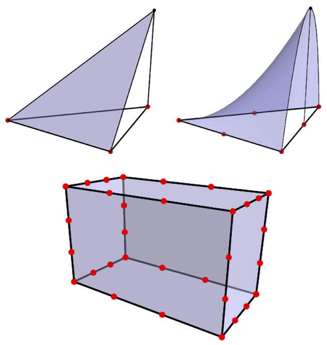
2.9. Neumann Spectrum

To demonstrate that Neumann spectra can be used to pick up significant geometric features much faster than Dirichlet spectra the eigenvalues of the cube with a tail (see Figure 8, left) were computed for the Neumann and the Dirichlet boundary condition and compared to the values of the cube. Figure 8 (right) shows the differences of the first 150 eigenvalues for the two different boundary conditions. Since the cube with tail has a larger volume, its eigenvalues are expected to be smaller than the values of the cube (see Section 2.2 2.). This fact is reflected in the graph (Figure 8 right) where the differences are always positive. It can be clearly seen that the Neumann spectrum picks up the differences much earlier than the Dirichlet spectrum. This is due to the fact that the Neumann boundary condition allows the solutions to oscillate at the boundary whereas the Dirichlet condition forces them to be zero on the boundary, strongly reducing their freedom especially in the region of the tail.

Fig. 8.

The first 150 eigenvalues of the cube with tail subtracted from the eigenvalues of the cube for the Dirichlet and Neumann case.

A 2D example of a square with a tail (S_T) illustrates the different behaviors of Neumann and Dirichlet boundary conditions. Figures 9 and 10 depict a comparison of a few eigenfunctions of the square with tail (S_T) and of the unit square (S₁) for both the Dirichlet and the Neumann case. For the Dirichlet case (Figure 9), the lower eigenfunctions do not detect the attached tail (9 a,e and b,f). For higher frequencies the nodal domains shrink (9 c,g) until they are finally able to slip into the smaller features. Because of the restrictive Dirichlet boundary condition, this only occurs around the 18th eigenfunction. From a signal processing point of view it is sensible that functions with higher frequencies can be used to analyze smaller features.

Fig. 9.

Eigenfunctions for Dirichlet boundary conditions for a square (top) and a square with tail (bottom). Low frequency (low eigenvalue) eigenfunctions do not probe the tail region due to the restrictive Dirichlet boundary conditions. Differences are picked up for high frequencies only where the higher spatial frequencies of the eigenfunctions allow for a probing of the tail region.

Fig. 10.

Eigenfunctions for Neumann boundary conditions for a square (top) and a square with a tail (bottom). Differences between the shapes are picked up already for small eigenvalues, since the Neumann boundary conditions allow the tail to swing freely for low frequencies.

The Neumann spectrum behaves differently (Figure 10). Because of the higher degree of freedom (with respect to the free vibration of the eigenfunctions at the boundary), small features like the tail influence the eigenfunctions already very early. It is unnecessary to compare the smallest eigenvalue which is always zero with constant eigenfunctions. But already the first non-constant eigenfunction (10 d) is very different from the first non-constant eigenfunctions of the square (10 a) since the extremum is shifted into the tail. This is reflected in a change of more than 50% of the corresponding eigenvalue. The next eigenfunction (10 e) of S_T on the other hand is zero in the tail region and therefore almost identical with (10 a). The corresponding eigenvalues are almost the same. Also the next few eigenfunctions (10 b ↔ f and c ↔ g) correspond with each other on the square region.

2.10. Influence of Noise

As demonstrated in Section 2.7, volume normalizations can lead to good spectral alignments. Nevertheless, having identical noise levels for the shape populations under investigation is essential, since different noise levels will affect surface areas differently (high noise levels yield highly irregular bounding surfaces especially if the voxel resolution is low). Because surface area is contained in the spectrum this has an influence on the eigenvalues. Violating the assumption of similar noise levels therefore leads to the detection of noise level differences as opposed to shape differences, as demonstrated in Figure 11 for noisy spheres (surfaces) and Figure 12 where the spectra of the ball (solid) are depicted with different levels of added noise. A fixed probability for adding a voxel to or removing a voxel from the object boundary was chosen for each experiment. Only voxels maintaining 6-connectivity were added or removed, guaranteeing a single 6-connected solid component. Increasing the noise level moves the corresponding spectra further apart. It can be seen in Figure 12 that the ball cannot be accurately represented with only a low voxel resolution, especially with high noise levels, the spectra move far apart. Such a noisy ball could also be seen as a noisy cube. For the analysis of identically acquired and processed shapes – e.g., obtained through manual segmentations of MRI (magnetic resonance image) data – a similar noise level is a reasonable assumption; we also assume the accuracy of the spectra calculations to stay the same for the whole population.

Fig. 11.

Spectra of a sphere with different noise levels. The noise-free case on the left demonstrates the accuracy of the numerical eigenvalue computations. Spectra were normalized to unit surface area. Black horizontal lines: analytic spectrum of the noise-free sphere. Increasing levels of noise from left to right.

Fig. 12.

Influence of noise on the ball spectrum (Dirichlet). Noise-levels influence the spectral signature of a shape.

2.11. Influence of the Discretization

Domain discretizations can significantly affect computational results. Figure 13 shows a two-dimensional example for a domain consisting of a small and a large square connected by a thin rectangle. Insufficient degrees of freedom, due to a coarse discretization, can lead to insufficiently resolved vibrational modes. In particular, thin structures may simply be overlooked if not enough nodes are contained in them. The Neumann spectra are not influenced as strongly by the discretization, as they allow free nodes on the boundary.

Fig. 13.

Eigenmode 19 for Dirichlet boundary conditions for different mesh refinements. Eigenmode contributions may be overlooked for coarse discretizations (left) in comparison to a fine discretization (right). In particular, thin structures may not get sufficiently probed for coarse discretizations.

3. Topological Analysis of Eigenfunctions

Eigenfunctions are real valued functions defined on the whole manifold. They are more difficult to deal with than eigenvalues but can be studied with topological methods, for example analyzing level sets and critical points. For the topological analysis of eigenfunctions we will construct the Morse-Smale (MS) complex on 2D surface representations and the Reeb graph inside the 3D voxel volume.

The MS complex [39,22] splits the domain of a function h into regions of uniform gradient flow. Its edges are specific integral lines (maximal paths on the surface and whose tangent vectors agree with the gradient of h) that run from the saddles to the extrema. For the construction of the MS complex for piecewise linear functions on triangulated surfaces see [11], where the concept of persistence is also described. It can be used, for example, to remove topological noise from the complex by pairing and canceling saddle/extrema combinations.

The MS complex is closely related to the Reeb graph [33], that captures the evolution of the level set components of the function and is often used in shape analysis applications. A level set is the pre-image h⁻¹(x) for a specific level x ∈ ℝ. The Reeb graph of a function h is obtained by contracting the connected components of the level sets to points. Thus the branching points and leaves (end points) in a Reeb graph correspond to level set components that contain a critical point of h. The leaves are the extrema while the branching points are saddles, where one edge is split into two (or more) or where edges are merged. The other points can be considered to lie on the edges between leaves and branching points. Note that the Reeb graph is a one-dimensional topological structure (a graph) with no preferred way of drawing it in the plane or space or attaching it to M (as opposed to the MS complex). Its edges are often manually attached to the shape by selecting the center of the represented level set.

Both the MS complex and the Reeb graph have been extensively used for shape processing and topological simplification. E.g. the MS complex has been constructed for a user selected eigenfunction of the mesh Laplacian for the purpose of meshing in [10].

So why is it of interest to study the eigenfunctions at all? In fact in addition to their relation to the corresponding eigenvalue (as demonstrated in the examples) they have some interesting properties. They are also isometry invariant and change continuously when the shape is deformed (although when ordered according to the magnitude of their eigenvalues, the ordering might switch). The functions with the smallest eigenvalues are more robust against shape change or noise, as they present the lower frequency modes. Another feature is their optimal embedding property used in manifold learning (see [3]). For example the first non-constant eigenfunction gives the smoothest embedding of the shape to the real line (of course complying with the boundary condition).

We will employ the eigenfunctions to give an indirect registration of similar shapes. As the (lower) eigenfunctions are stable across the shapes, they have similar values in similar location. Thus, we can measure local shape differences by analyzing landmarks such as lengths of level sets or integral lines, or areas of level surfaces in 3D. A simple example is given Figure 14 where two planar domains are shown together with their first eigenfunctions (color shaded) and level sets. The two domains where modeled with the medial modeler by adjusting the medial axis and the thickness function and then processed (meshed, FEM computation …) as described in [44]. It can be seen how the extrema and level sets are at similar locations for both shapes, even though bending and thickness changes are involved. The length of the level sets can be used to do a thickness comparison. We will demonstrate similar comparisons later for 3D solids. The Reeb graph is a line from the minimum to the maximum running through the midpoints of each level set and can be used to measure length. For the simple example in Figure 14 the MS complex cannot be constructed as no saddles are involved. However, the MS complex will be helpful for studying higher eigenfunctions on surfaces, where additional interesting features such as saddles and multiple extrema exist.

Fig. 14.

First non-constant eigenmode for two similar shapes. Red and blue dots at the tips denote the extrema, the green curves are some level sets. The Reeb graph (gray curve) approximates the medial axis.

4. Statistical Analysis of Groups of LB Spectra

The (possibly normalized) beginning sequence of the Laplace-Beltrami spectrum (called ShapeDNA) can be interpreted as a point $\mathit{v}\in {\mathbb{R}}_{\ge 0}^n$ in the n-dimensional positive Euclidean space. Given the ShapeDNA v_i of many individual objects divided into two populations A and B we use permutation tests to compare group features to each other (200,000 permutations were used for all tests). We call a set of objects the object population. Permutation testing is a nonparametric, computationally simple way of establishing group differences by randomly permuting group labels. Let S_A = {v_i} and S_B = {v_j} denote two sets of ShapeDNA associated to individuals for group A and for group B respectively. Assume for example that we want to investigate if elements in S_A have on average a larger Euclidean norm than the elements in S_B (due to some external influences). A possible test statistic stat would be the sum of the lengths of the elements in S_A (stat:= Σ_vi∈SA||v_i||). For the permutation test we then randomly distribute the subjects into groups A and B, keeping the number of elements per group fixed. We define the p-value to be the fraction of these permutations having a greater or equal sum stat than the original set S_A (in other words the relative frequency of occasions where the random label outperforms the original labeling). The values of S_A will be considered significantly larger than the ones of S_B at a prespecified significance level α if p ≤ α (taken as α = 5% here). Note, that rejecting the null hypothesis of two populations being equal given a significance level α only implies that the probability of making a type I error (i.e., the probability of detecting false positives; “detecting a difference when there is none in reality”) is α, but does not exclude the possibility of making such an error.

Confidence intervals for the estimated p-values p̂ may be computed following Nettleton et al. [26] for 100(1 − γ)% confidence as

$$\begin{array}{l}(\widehat{p}-{\mathrm{\Psi }}^{-1}(1-\frac{\gamma }{2})\sqrt{\widehat{p}(1-\widehat{p})/N},\\ \widehat{p}+{\mathrm{\Psi }}^{-1}(1-\frac{\gamma }{2})\sqrt{\widehat{p}(1-\widehat{p})/N})\end{array}$$

where

$${\mathrm{\Psi }}^{-1}(x)=\sqrt{2}er{f}^{-1}(2x-1)$$

is the inverse of the cumulative distribution function of the standard normal distribution, erf⁻¹(·) is the inverse error function, N denotes the number of samples (200,000 in our case). The approximation is based on the binomial distribution and holds for Np ≥ 5. Figure 15 shows the confidence intervals for a confidence range of [90%, 99%] for p-values p ∈ {0.0001, 0.05}. Note, that the plots are the same, except for scaling, which depends only on the different p-values. While these are just probabilistic characterizations of the confidence in the estimated p-value they demonstrate that using 200, 000 permutations will give good estimations up to the first or even the second non-zero decimal place.

Fig. 15.

Confidence intervals for p ∈ {0.0001, 0.05} with N = 200, 000 permutations

We use three different kinds of statistical analyses (all shapes are initially corrected for brain volume differences, also see [14] for details on permutation testing):

1. A nonparametric, permutation test to analyze the scalar quantities: volume and surface area.

2. A nonparametric, multivariate permutation test based on the maximum t-statistic to analyze the high-dimensional spectral feature vectors (Shape-DNA in 2D and 3D cases).

3. Independent permutation tests of the spectral feature vector components across groups (as in (2)), followed by a false discovery rate (FDR) approach to correct for multiple comparisons, to analyze the significance of individual vector components.

To test scalar values the absolute mean difference is used as the test statistic s = |μ_a−μ_b|, where the μ_i indicates the group means. The maximum t-statistic is chosen due to the usually small number of available samples in medical image analysis, compared to the dimensionality of the ShapeDNA feature vectors (preventing the use of the Hotelling T² statistic [17]). It is defined as

$$\mathit{stat}=t_{\mathit{max}}:=\underset{1\le j\le N}{\mathit{max}}\frac{|{\overline{\mathit{v}}}_{A,j}-{\overline{\mathit{v}}}_{B,j}|}{S{E}_j}.$$ (21)

Here, N is the vector dimension, v¯_A,j indicates the mean of the j-th vector component of group A, and SE_j is the pooled standard error estimate of the j-th vector component, defined as

$$S{E}_j=\frac{\sqrt{(n_A-1){\sigma }_{A,j}^2+(n_B-1){\sigma }_{B,j}^2}}{\sqrt{\frac{1}{n_A}+\frac{1}{n_B}}},$$ (22)

where n_i is the number of subjects in group i (with i ∈ A,B) and σ_i,j is the standard deviation of vector component j of group i. The maximum t-statistic is particularly sensitive to differences in at least one of the components of the feature vector [5]. It is a summary statistic, which allows for the detection of differences between feature vectors across populations. However, it does not determine which components show statistically significant differences.

Nevertheless, testing the individual statistical significance of vector components is possible. Such testing needs to be performed over a whole set of components, since it is usually not known beforehand which component of a ShapeDNA vector will be a good candidate for statistical testing. (I.e., we can in general not simply pick one individual vector component (eigenvalue) for statistical testing.) To account for multiple comparisons when testing over a whole set of vector components, the significance level needs to be adjusted (since “the chance of finding differences that are purely random in nature increases with the number of tests performed”). See [12,14] for background on schemes for multiple comparison corrections.

5. Results

Volume measurements are the simplest means of morphometric analysis. While volume analysis results are easy to interpret, they only characterize one morphometric aspect of a structure. The following Sections describe the Laplace-Beltrami and the volumetric Laplace spectrum as a method for a more complete global structural description using the analysis of a caudate as an exemplary brain structure. Note, that it makes sense to look at the 2D surface and at the 3D solid as the spectra of the surfaces contain other information than the solid spectra. In [37] examples of iso-spectral 3D solids (orthogonal “GWW” prism) were presented, where the spectral analysis of their 2D boundary shells was capable of distinguishing the shapes.

For brevity all results are presented for the right caudate only.

5.1. Populations and Preprocessing

Magnetic Resonance Images (MRI) of the brains of thirty-two neuroleptic-naïve female subjects diagnosed with Schizotypal Personality Disorder (SPD) and of 29 female normal control subjects were acquired on a 1.5-T General Electric MR scanner. Spoiled-gradient recalled acquisition (SPGR) images (voxel dimensions 0.9375 × 0.9375 × 1.5 mm) were obtained coronally. The images were used to delineate the caudate nucleus (see Figure 16) and to estimate the intracranial content (ICC) used for volume normalization to adjust for different head sizes. For details see [23].

Fig. 16.

Example of a caudate shape consisting of cuboid voxels (left). Exemplary caudate surface shape unsmoothed and with spherical harmonics smoothing (right).

The caudate nucleus was delineated manually by an expert [23]. For the 2D surface analysis the isosurfaces separating the binary labelmaps of the caudate shapes from the background were extracted using marching cubes (while assuring spherical topology). Analysis was then performed on the resulting triangulated surface directly (referred to as unsmoothed surfaces in what follows) as well as on the same set of surfaces smoothed and resampled using spherical harmonics³ (referred to as smoothed surfaces in what follows). The unsmoothed surfaces are used as a benchmark dataset subject to only minimal preprocessing, whereas the smoothed surfaces are used to demonstrate the influence of additional preprocessing. See Figure 16(right) for an example of a smoothed and an unsmoothed caudate.

5.2. Volume and Area Analysis

For comparison, results for a volume and a surface area analysis are shown in Figure 17. As has been previously reported for this dataset [23], subjects with schizotypal personality disorder exhibit a statistically significant volume reduction compared to the normal control subjects. While smoothing plays a negligible role for the volume results (smoothed: p = 0.008, volume loss 7.0%, i.e., there is a chance of p = 0.008 that the volume loss is a random effect; unsmoothed: p = 0.013, volume loss 6.7%), the absolute values of the surface area are affected more, since smoothing impacts surface area more than volume. The results for the female caudates show the same trend for the surface areas in the smoothed and the unsmoothed cases.

Fig. 17.

Group comparisons for volume differences (top) and surface area differences (bottom). Smoothed results prefix ‘s’, unsmoothed results prefix ‘us’. Volume and surface area reductions are observed for the SPD population in comparison to the normal control population.

5.3. Laplace-Beltrami Spectrum Results (2D Surface)

The LB spectrum was computed for the female caudate population (on the surfaces) using the two different normalizations:

1. The shapes were volume normalized to unit intracranial content (UIC) (using the ICC measurements) to account for different head sizes.

2. The shapes were normalized to unit caudate surface area (UCA) to analyze shape differences independently of size.

A maximum t-statistic permutation test on a 100-dimensional spectral shape descriptor shows significant shape differences (see Table 1) for caudate surface area normalization for the unsmoothed surfaces, but not for the smoothed ones. Surface area normalization is the strictest normalization in terms of spectral alignment. Testing for surface area independently yields statistically significant results, listed in Table 1.

Table 1.

Shape comparison results for the maximum t-statistic permutation test for the unsmoothed (US) and smoothed (S) dataset. Volume and area results for comparison. The used normalizations are: unit intracranial content (UIC), unit caudate surface area (UCA) and unit caudate volume (UCV).

	norm	p-value (US)	p-value (S)
LBS (N=20)	UIC	0.0026	0.0013
	UCA	0.005	0.63
LBS (N=100)	UIC	0.0003	0.0009
	UCA	0.026	0.84
Volume	UIC	0.013	0.0078
	UCA	0.0011	0.011
Area	UIC	0.0001	0.0002
	UCV	0.001	0.011

Figure 18 indicates that using too many eigenvalues has a slightly detrimental effect on the observed statistical significance. This is sensible, since higher order modes correspond to higher frequencies and are thus more likely noise, which can overwhelm the statistical testing. It is thus sensible to restrict oneself only to a subset of the spectrum (e.g., the first twenty). However, this subset needs to be agreed upon before the testing and cannot be selected after the fact. Note, that the Laplace-Beltrami-Spectrum results of Table 1 show statistically significant shape differences even when the strong influence of surface area is removed, which suggests that the Laplace-Beltrami-Spectrum indeed picks up shape differences that complement area and volume findings. The Laplace-Beltrami-Spectrum can detect surface area differences (since the surface areas may be extracted from the spectrum) and can distinguish objects with identical surface area or volume based on their shape.

Fig. 18.

Maximum t-statistic results of area normalized case (top) for the first n eigenvalues, i.e. shape-DNA’s of different length, (solid line: unsmoothed, dashed line: smoothed) and (bottom) for individual eigenvalues (unsmoothed case) with FDR multiple comparison correction. The black horizontal lines correspond to the 5% significance level and the 5% FDR corrected significance level respectively. Since the statistically most significant eigenvalue cannot be selected after the statistical analysis, a shape-DNA-based analysis with prespecified length is useful.

It should be noted that tests with the twelve invariant moments (invariant with respect to similarity group actions) as proposed in [20] did not yield statistically significant shape differences for the caudate shape population, showing that the spectrum has more discrimination power here (as the first few eigenvalues are sufficient to detect differences between the groups).

5.4. Laplace-Beltrami Eigenfunctions (2D Surface)

To explore why some of the eigenvalues are statistically significant, we investigate their associated eigenfunctions. This will also guide our search for new shape descriptors based on the eigenfunctions of the Laplace Betrami operator. In Fig. 18 (bottom) the eigenvalue λ₂ has a low p-value of 0.0003. Since the caudate shapes are rather long and thin, not only the gradients of the first non-zero eigenfunction, but also of the second are aligned with the general direction of the caudate shape.

It can be seen in Figure 19 that the first non-constant eigenfunction (right) has extrema at the two ends of the shape. Due to its simplicity it is not very descriptive, but maps the shapes nicely to the real line along its main direction, thus giving an implicit registration along their main trend. The second eigenfunction (left and middle) has two maxima at the tips of the shape, one minimum at the outer rim and a saddle in the middle of the inner rim. The green curves denote the nodal lines (zero level sets) and the blue and red curve are constructed by following the gradient from the saddle up to the maxima (red) and down to the minimum (blue), thus constructing the Morse-Smale complex (see Section 3).

Fig. 19.

Left and middle: Eigenfunction (EF) 2 with maxima at tips (red), minimum at outer rim (blue, middle) and saddle at inner rim (green, left), the integral lines (red and blue curve) run from the saddle to the extrema. Right: EF 1 with extrema at the tips and no saddle. The closed green curves denote the zero level sets (two for EF 2 and only one for EF 1).

The second eigenfunction captures the main direction of the shape, which can be seen nicely at the green nodal lines and the blue curve being orthogonal to the main direction and spread well apart. Additionally, the second eigenfunction captures the thickness as the minimum and the maxima are located at opposing rims of the shape. As all the caudates in this population are of similar shapes, this behavior is true for all of them. In some cases we have an additional saddle-minimum pair at the outer rim that can be identified as topological noise induced by the mesh (see Fig. 20). Such noisy pairs can be detected and canceled using the concept of persistence [11] pairing related extrema/saddle combinations according to their significance.

Fig. 20.

Noisy Morse-Smale complex of the second non constant eigenfunction on the outer rim (left) and close-up (middle). After canceling the saddle with the closest minimum, only one minimum remains and the red integral lines from the saddle to the two maxima at the head and tail disappear.

To analyze the shapes we performed the statistical test on the following descriptors:

• (hc) the head circumference (long green curve)

• (wc) the waist circumference (blue curve)

• (tc) the tail circumference (short green curve)

• (l) the length (red curve).

We obtained the following p-values for the unit intracranial content (UIC) and the unit caudate surface area (UCA) normalized cases:

	UIC	UCA
hc	p = 0.0015	p = 0.45
wc	p = 0.0016	p = 0.053
tc	p = 0.007	p = 0.039
1	p = 0.21	p = 0.0003

The statistically significant cases are printed in bold. For the intracranial content normalized case significant differences are detected in all the three circumferences, but not in the lengths of the shape. The caudate surface area normalization principally reverses the results. This could be expected as the main surface area lies in the shell of these cylindrical shapes and not at the cylinder caps. Therefore a surface area normalization seems to adjust the circumferences and changes the lengths instead. Nevertheless, we still pick up statistically significant differences in the tail region of the shapes (which can also be expected as the head has more surface area than the tail).

The intracranial content normalized results suggest that shape differences are mainly in shape thickness as opposed to shape length. Figure 21 shows a group comparison of the waist circumferences (top) of the ICC normalized shapes, as well as the differences in length after caudate area normalization (bottom). Note also that in the unit caudate area case, the length indicates an increase in mean distance between the nodal lines. This explains why the corresponding eigenvalue is also significantly smaller for the SPD population (as it is related to the frequency of the oscillation, which is related to the size of the oscillating domains).

Fig. 21.

Group comparisons for waist circumferences differences (left) and length differences (right) after caudate area normalization. A waist length reduction can be observed for the SPD population in comparison to the normal controls (unit ICC). After caudate area normalization, an increase in length can be seen.

Similar to Figure 14 it is possible to wrap more level sets around the caudate shapes (see Fig. 22), with the difference that now we get closed curves. Again the level sets yield an indirect registration of the shapes and present a method to detect local circumference differences. Note that we could actually construct a common parametrization (e.g. on the sphere) by taking the level and the position on the closed level set as the two parameters, but this explicit parametrization is not needed. Figure 23 shows a plot of the level set lengths of a few caudate shapes. The p-value for the whole population can be found in Figure 24 and indicate that not only the thinner regions in the tail (level 0.2) are significantly different, but also the region at the beginning of the head (level 0.7) show highly significant differences.

Fig. 22.

100 level sets wrapped around two exemplary caudate shapes using the first eigenfunction. The absence of any saddles guarantees that each level set has only one component.

Fig. 23.

Lengths of level sets (mapped onto the unit interval) of 8 exemplary shapes (sampling at 200 levels). Red curves: SPD subjects, green curves: normal controls.

Fig. 24.

p-value for the whole population on each level set (sampling at 200 levels). The red line marks the significance level corrected for multiple comparisons (FDR).

5.5. Laplace Spectrum Results (3D Solid)

As we deal with 3D solid objects it makes sense to also look at the solid instead of analyzing the surface only. The Laplace spectrum of the 3D voxel data was computed for two different normalizations:

1. The shapes were volume normalized to unit intracranial content (using the ICC measurements) to account for different head sizes.

2. The shapes were normalized to unit caudate volume to analyze shape differences independently.

In order to get more inner nodes especially into the very thin tail region of the caudate shapes we additionally employed the dual of the voxel graph. The dual voxel graph is the voxel image where each voxel of the original image (regular voxel image) is considered to be a vertex of the dual graph. Voxels inside the domain become inner vertices while voxel just outside of the domain’s boundary now become boundary vertices. Figure 25 depicts a 2D case (using pixels) with the original regular domain on the left and the dual on the right. The dual graph enlarges the domain by half a layer thus creating new inner nodes needed especially inside the thinner features (tail). The use of the dual graph is helpful since a global refinement of the voxels leads to large FEM models that may cause memory problems on some standard PC’s. Note that in 3D the number of voxels increases by the factor 8 for each refinement step, this will quickly get large, especially if a higher order FEM is used, needing many nodes per voxel. The main difficulty lies in solving the large eigenvalue problem as the LU decomposition (SuperLU libary) might require a lot of additional memory if a large amount of fill-ins is generated⁴.

Fig. 25.

Regular pixel domain (left) and its dual (right).

Since the two populations show significant differences in volume, surface area, local shape thickness and in their 2D surface spectra (see above), we expect to find significant differences also in their 3D volume spectra. The following paragraphs present first the Dirichlet, then at the Neumann spectrum results for both the regular and dual voxel graph.

5.5.1. Dirichlet Spectra

Figure 26 shows the statistical results for the regular voxel graph and its dual for the caudate populations. The graph shows the corresponding p value (see Section 4) when using the first N eigenvalues of the spectra for the statistical analysis (unit intracranial content). Recall that not just a single eigenvalue is used but the whole beginning sequence of the first N values (therefore we call these plots accumulated statistic plots). A p value below the 5% horizontal line is considered to be statistically significant. In such a case the beginning sequence of the spectrum is considered to be able to distinguish between the two caudate populations (NC and SPD). Figure 26 shows that the beginning sequence of the Dirichlet spectrum does not yield any statistically significant results. Employing the dual graph yields lower p-values when higher eigenvalues get involved. This observation is sensible, considering the fact that especially in the thin tail part of the caudates only very few inner nodes exist (see Section 2.11 for the effects of low resolution). The dual graph has more degrees of freedom, introducing inner nodes in the thin tail area, and therefore improves the result. In unit caudate volume case we did not find any significant differences either. For a detailed analysis employing the Dirichlet spectrum higher voxel resolutions would be necessary. Due to the low voxel resolution the computed eigenfunctions do not seem to accurately represent the real eigenfunctions of the caudate shapes.

Fig. 26.

Accumulative maximum t-statistic results (unit intracranial content, Dirichlet) for the regular (left) and the dual (right) voxel graphs. Employing the dual graph yields lower p-values. This may be attributed to the better suitability of the dual graph for probing the thin tail regions of the caudate shapes. However, there is no statistical difference at a significance level of α = 5%.

5.5.2. Neumann Spectra

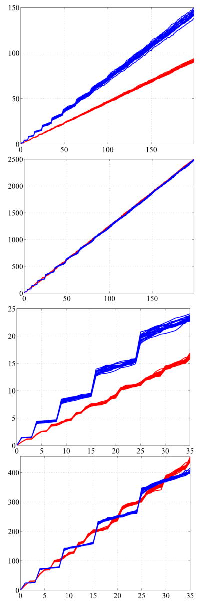
As demonstrated in section 2.9, the Neumann spectrum can help to identify shape differences much earlier than the Dirichlet spectrum. Figure 27 shows the accumulated statistics plots for different normalizations of the Neumann spectra for the regular and the dual case. In both cases (regular and dual) the intracranial content normalized spectra show very similar behavior (27 a,b): already very early, significant differences are detected. Because these differences might simply reflect the different caudate volumes (known to be significant) a normalization to unit caudate volume (27 c,d) is applied to reveal volume-independent shape differences. The eigenvalues in the regular case (27 c) do not show statistically significant shape differences until about 150 eigenvalues are involved, however, the dual case (27 d) shows a significant p value already for 50 or more eigenvalues used. The reason seems to be that the higher frequency eigenfunctions have smaller nodal domains and can thus better detect the smaller features, presumably in the tail region. This assumption aligns with the Dirichlet case (Figure 26 dual) where better p-values are obtained when employing higher frequencies.

Fig. 27.

Accumulated statistic, Neumann boundary conditions. Statistically significant shape differences are detected as expected for the unit intracranial content cases (a and b) (due to the caudate volume differences between the SPD and the NC populations). After caudate volume normalization (c and d), differences are first detected for the dual graph analysis (d), presumably because the additional degrees of freedom enable a proper probing of the caudate tail regions.

The accumulated results in Fig. 27 can be partially explained by analyzing the p-values of the individual eigenvalues (see Fig. 28). It can be seen that the p-value of the eigenvalue λ₅ is very low in both the regular and the dual voxel graphs (marked in red). This leads to significant results very early in the accumulated plots. Furthermore, the low p-values around the 50th eigenvalue (the 52nd in particular, also marked in red) in the dual case seem to produce the significant results in the accumulated plots above.

Fig. 28.

p-values for the individual eigenvalues with Neumann boundary condition for the regular (top) and dual (bottom) voxel graph.

5.6. Laplace Eigenfunctions (3D Solid)

Similar to the analysis of interesting eigenfunctions in the 2D surface case it makes sense to analyze the eigenfunctions in 3D. By looking at the nodal surfaces (zero level sets) of the eigenfunctions λ₅ and λ₅₂ (Fig. 29) it can be noticed that these eigenfunctions, whose gradient field is always orthogonal to the nodal surfaces, again follow the main trend of the shape (for the 52nd function only in the tail region). We focus on the 5th eigenfunction (due to its simplicity) and analyze its nodal surfaces with respect to two hypotheses. As can be seen in the example in Figure 29, the nodal surfaces of the 5th eigenfunction are usually 4 separated components (true in all except for 3 cases). First we want to relate the eigenfunction to the significant eigenvalue. As the eigenvalues are the square roots of the frequencies of the oscillation, the size of the nodal domains and therefore the distances of the nodal surfaces (green lines in Figure 29 bottom) should yield significant results after the caudate volume normalization. Furthermore, we know from the 2D analysis that significant changes in thickness (before caudate area normalization) are present mainly in the tail region of the shapes. Therefore, we will test the hypotheses that

Fig. 29.

Nodal surfaces of eigenfunction 52 (top) and 5 (bottom), where the centroids are connected.

1. the mean distance of the nodal surfaces (l1) on the unit volume caudates are larger for the SPD population (leading to a smaller eigenvalue EV5).

2. the mean boundary length (l2) and the mean surface area (l3) of the small nodal surface components in the tail region (removing the large component in the head) are smaller for the SPD population.

For the first experiment, we compute the barycenter of the vertices of each nodal surface component and use it as a representation of that component. We then connect neighboring components with each other (green line in Fig. 29 bottom) and compute the mean distance between neighboring components. Note that the green line is a skeletal representation of the shape. In fact, it is the Reeb graph [33], as each level set component is represented by a node (red dot) which is connected to its neighbors by the green edges. Thus, this skeletal model represents the topological structure of the analyzed eigenfunction EV5 which yields an interesting shape descriptor, that could be used for other application, such as non-rigid registration. For both experiments we obtained the following p-values for the unit intracranial content (UIC) and unit caudate volume (UCV) cases:

	UIC	UCV
l1	p = 0.21	p = 0.0099
l2	p = 0.0001	p = 0.0003
l3	p = 0.0019	p = 0.015

For the first experiment we have significant values for the mean distances of the nodal surfaces after caudate volume normalization. We detect an increase in length for the SPD population, which goes in line with the significant decrease of the 5th eigenvalue, related to the size of the nodal domains (see Figure 30). All the values for l2 and l3 are statistically significant, where especially the mean boundary lengths (similar to the waist and tail circumferences in 2D) are highly significant (see also Figure 31 for the direct comparison of the boundary lengths in the UIC case).

Fig. 30.

Group comparison for the eigenvalue 5 (left) and mean distance of the nodal surfaces (right) for the unit intracranial content. A reduction of the eigenvalue and a corresponding increase of the distances can be observed for the SPD population in comparison to the normal controls.

Fig. 31.

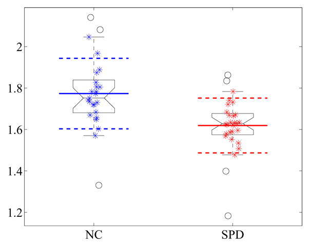
Group comparison for the boundary length of the small nodal surfaces for the unit intracranial content. A reduction can be observed for the SPD population in comparison to the normal controls.

6. Conclusion

This paper describes methods for global and local shape analysis using the Laplace-Beltrami eigenvalues and eigenfunctions with Dirichlet and Neumann boundary conditions for 2D surfaces (triangle meshes) and 3D volumetric solids (voxel data). The eigenvalues and -functions including their geometric and topological features are defined invariantly wrt. mesh, location, parametrization and depend on the isometry type only. Our experiments corroborate their robustness wrt. noise. We demonstrated their discrimination power successfully at a real application in medical imaging to distinguish populations of similar shapes.

The Laplace-Beltrami eigenvalues are well suited as a global shape descriptor, without the need to register the shapes. They could successfully be employed to detect true shape differences of the two populations (using the maximum t-statistic) even after normalization hinting at caudate shape differences in Schizotypal Personality Disorder. It could be demonstrated that the volumetric Neumann spectra can detect statistically significant shape differences when applied directly to the voxel data. These computations are feasible on a standard desktop computer. The Neumann spectra are of interest, since they recognize shape differences much earlier than the Dirichlet spectra and also work much better if the voxel resolution is very low. Especially the higher eigenvalues yield statistically significant results, indicating true shape differences mainly in areas with smaller features.

Additionally, we proposed a novel method to employ the eigenfunctions on surfaces for the detection and registration of features across shapes. We introduced a topological analysis (Morse-Smale complex and nodal curves) of selected eigenfunctions to define geometric features and to localize shape differences (here the local thickness of the caudate shapes). Also the topological analysis of eigenfunctions in 3D data is new and yields interesting geometric entities (distance, boundary length and surface areas of nodal surfaces) which underline the shape differences in the presented application (thickness differences and length differences for the unit volume caudates). These geometric properties also contribute towards an interpretation of the corresponding eigenvalues.

The presented results are promising and show that the spectra (eigenfunctions and eigenvalues) of the Laplace-Beltrami operator are capable shape descriptors, especially when combined with a topological analysis, such as locations of extrema, behavior of the level sets and the construction of the Morse-Smale complex (or Reeb graph). The presented methods are expected to be applicable in other settings. Future work will focus on the possibility to compare shape based on a specific size of the features of interest (multiresolution shape matching), founded on the frequency analysis delivered by the Laplace spectra. Another direction of research will be the non-rigid registration of shapes employing eigenfunctions and their topological features. Furthermore, it is of interest to construct generalized feature vectors consiting of 2D and 3D (geometric and topological, global and local) features for the fast comparison of shapes or the retrieval of objects from large shape databases.

References

- 1.Angenent S, Haker S, Tannenbaum A, Kikinis R. Laplace-Beltrami operator and brain surface flattening. IEEE Trans Medical Imaging. 1999;18:700–711. doi: 10.1109/42.796283. [DOI] [PubMed] [Google Scholar]
- 2.ARPACK, Arnoldi package, http://www.caam.rice.edu/software/ARPACK/.
- 3.Belkin M, Niyogi P. Laplacian Eigenmaps for dimensionality reduction and data representation. Neural Computations. 2003;15(6):1373–1396. [Google Scholar]
- 4.Blaschke W, Leichtweiss K. Elementare Differentialgeometrie. Springer Verlag; 1973. [Google Scholar]
- 5.Boyett JM, Shuster JJ. Nonparametric one-sided tests in multivariate analysis with medical applications. Journal of the American Statistical Association. 1977;72(359):665–668. [Google Scholar]
- 6.Braess D. Finite Elemente. Springer Verlag; 1997. [Google Scholar]
- 7.Chavel I. Eigenvalues in Riemannian Geometry. Academic Press; 1984. [Google Scholar]
- 8.Courant R, Hilbert D. Methods of Mathematical Physics. Interscience. 1953;I [Google Scholar]
- 9.Demmel JW, Eisenstat SC, Gilbert JR, Li XS, Liu JWH. A supernodal approach to sparse partial pivoting. SIAM J Matrix Analysis and Applications. 1999;20(3):720–755. [Google Scholar]
- 10.Dong S, Bremer PT, Garland M, Pascucci V, Hart JC. Spectral surface quadrangulation. ACM SIGGRAPH 2006. 2006:1057–1066. [Google Scholar]
- 11.Edelsbrunner H, Harer J, Zomorodian A. Hierarchical Morse-Smale complexes for piecewise linear 2-manifolds. Discrete and Computational Geometry. 2003;30(1):87–107. [Google Scholar]
- 12.Genovese CR, Lazar NA, Nichols T. Thresholding of statistical maps in functional neuroimaging using the false discovery rate. Neuroimage. 2002;15:870–878. doi: 10.1006/nimg.2001.1037. [DOI] [PubMed] [Google Scholar]
- 13.Gerig G, Styner M, Jones D, Weinberger D, Lieberman J. Shape analysis of brain ventricles using spharm. Proceedings of the Workshop on Mathematical Methods in Biomedical Image Analysis (MMBIA); 2001. pp. 171–178. [Google Scholar]
- 14.Good P. Permutation, Parametric, and Bootstrap Tests of Hypotheses. 3. Springer; 2005. [Google Scholar]
- 15.Gordon C, Webb D, Wolpert S. Isospectral plane domains and surfaces via riemannian orbifolds. Inventiones Mathematicae. 1992;110:1–22. [Google Scholar]
- 16.Grimes RG, Lewis JG, Simon HD. A shifted block Lanczos algorithm for solving sparse symmetric generalized eigenproblems. SIAM Journal on Matrix Analysis and Applications. 1994;15(1):228–272. [Google Scholar]
- 17.Hotelling H. The generalization of student’s ratio. The Annals of Mathematical Statistics. 1931;2(3):360–378. [Google Scholar]
- 18.Levitt J, Westin CF, Nestor PG, Estepar RSJ, Dickey CC, Voglmaier MM, Seidman LJ, Kikinis R, Jolesz FA, McCarley RW, Shenton ME. Shape of the caudate nucleus and its cognitive correlates in neuroleptic-naive schizotypal personality disorder. Biological Psychiatry. 2004;55:177–184. doi: 10.1016/j.biopsych.2003.08.005. [DOI] [PMC free article] [PubMed] [Google Scholar]
- 19.Mamah D, Wang L, Barch D, de Erausquin G, Gado M, Csernansky J. Structural analysis of the basal ganglia in schizophrenia. Schizophrenia Research. 2007;89(1–3):59–71. doi: 10.1016/j.schres.2006.08.031. [DOI] [PMC free article] [PubMed] [Google Scholar]
- 20.Mangin JF, Poupon F, Duchesnay E, Riviere D, Cachia A, Collins DL, Evans AC, Regis J. Brain morphometry using 3d moment invariants. Medical Image Analysis. 2004;8:187–196. doi: 10.1016/j.media.2004.06.016. [DOI] [PubMed] [Google Scholar]
- 21.McKean H, Singer I. Curvature and the eigenvalues of the laplacian. Journal of Differential Geometry. 1967;1:43–69. [Google Scholar]
- 22.Milnor J. Morse Theory, vol. 51 of Annals of mathematics studies. Princeton University Press; 1963. [Google Scholar]
- 23.Min-Seong K, Levitt J, McCarley RW, Seidman LJ, Dickey CC, Niznikiewicz MA, Voglmaier MM, Zamani P, Long KR, Kim SS, Shenton ME. Reduction of caudate nucleus volumes in neuroleptic-naive female subjects with schizotypal personality disorder. Biological Psychiatry. 2006;60:40–48. doi: 10.1016/j.biopsych.2005.09.028. [DOI] [PMC free article] [PubMed] [Google Scholar]
- 24.Nain D, Styner M, Niethammer M, Levitt J, Shenton ME, Gerig G, Bobick A, Tannenbaum A. Statistical shape analysis of brain structures using spherical wavelets. Proceedings of the International Symposium of Biomedical Imaging (ISBI); 2007. pp. 209–212. [DOI] [PMC free article] [PubMed] [Google Scholar]
- 25.Naff H, Wolter FE, Dogan C, Thielhelm H. Medial Axis Inverse Transform in 3-Dimensional Riemannian Complete Manifolds, in: Proceedings of the 2007 International Conference on Cyberworlds (NASAGEM) IEEE Computer Society. 2007:386–395. [Google Scholar]
- 26.Nettleton D, Doerge RW. Accounting for variability in the use of permutation testing to detect quantitative trait loci. Biometrics. 2000;56(1):52–58. doi: 10.1111/j.0006-341x.2000.00052.x. [DOI] [PubMed] [Google Scholar]
- 27.Niethammer M, Reuter M, Wolter F-E, Bouix S, Peinecke N, Koo M-S, Shenton ME. Global medical shape analysis using the Laplace-Beltrami spectrum. Conference on Medical Image Computing and Computer Assisted Intervention, Part I, LNCS 4791, Lecture Notes in Computer Science; Brisbane, Australia: Springer; 2007. pp. 850–857. [DOI] [PMC free article] [PubMed] [Google Scholar]
- 28.Peinecke N, Wolter FE, Reuter M. Laplace spectra as fingerprints for image recognition. Computer-Aided Design. 2007;39(6):460–476. [Google Scholar]
- 29.Peinecke N, Wolter F-E. Mass Density Laplace Spectra for image recognition. Proceedings of the 2007 Inernational Conference on Cyberworlds (NASAGEM), IEEE Computer Society; 2007. pp. 409–416. [Google Scholar]
- 30.Qui A, Bitouk D, Miller MI. Smooth functional and structural maps on the neocortex via orthonormal bases of the Laplace-Beltrami operator. IEEE Transaction on Medical Imaging. 2006;25(10):1296–1306. doi: 10.1109/tmi.2006.882143. [DOI] [PubMed] [Google Scholar]
- 31.Qiu A, Younes L, Miller MI. Intrinsic and extrinsic analysis in computational anatomy. NeuroImage. 2008;39(4):1803–1814. doi: 10.1016/j.neuroimage.2007.08.043. [DOI] [PubMed] [Google Scholar]
- 32.Rausch T, Wolter F-E, Sniehotta O. Computation of Medial Curves in Surfaces, in Conference on the Mathematics of Surfaces VII. Inst of Math and its Appl. 1997:43–68. [Google Scholar]
- 33.Reeb G. Sur les points singuliers d’une forme de Pfaff completement intgrable ou d’une fonction numrique. Comptes rendus de l’Acadmie des sciences, Paris. 1946;222:847–849. [Google Scholar]
- 34.Reuter M. Laplace Spectra for Shape Recognition, Books on Demand. Norderstedt; Germany: 2006. [Google Scholar]
- 35.Reuter M, Niethammer M, Wolter F-E, Bouix S, Shenton ME. Global medical shape analysis using the volumetric Laplace spectrum. Proceedings of the 2007 Inernational Conference on Cyberworlds (NASAGEM), IEEE Computer Society; 2007. pp. 417–426. [Google Scholar]
- 36.Reuter M, Wolter F-E, Peinecke N. Laplace-spectra as fingerprints for shape matching. SPM ‘05: Proceedings of the 2005 ACM Symposium on Solid and Physical Modeling; Cambridge, MA: ACM Press; 2005. pp. 101–106. [Google Scholar]
- 37.Reuter M, Wolter FE, Peinecke N. Laplace-Beltrami spectra as shape-DNA of surfaces and solids. Computer-Aided Design. 2006;38(4):342–366. [Google Scholar]
- 38.Shi Y, Lai R, Krishna S, Dinov I, Toga AW. Anisotropic laplace-beltrami eigenmaps: Bridging reeb graphs and skeletons. Computer Vision and Pattern Recognition Workshops, 2008. CVPR Workshops, IEEE Computer Society; Anchorage, AK. 2008. pp. 1–7. [DOI] [PMC free article] [PubMed] [Google Scholar]
- 39.Smale S. On gradient dynamical systems. Ann of Math. 1961;74:199–206. [Google Scholar]
- 40.Strang G, Fix GJ. An Analysis of the Finite Element Method. Prentice-Hall; 1973. [Google Scholar]
- 41.Styner M, Oguz I, Xu S, Brechbühler C, Pantazis D, Levitt J, Shenton ME, Gerig G. Framework for the statistical shape analysis of brain structures using spharm-pdm. Proceedings of the Open Science Workshop; MICCAI. 2006. [PMC free article] [PubMed] [Google Scholar]
- 42.Wolter FE. Distance Function and Cut Loci on a Complete Riemannian Manifold. Arch Math. 1979;32:92–96. [Google Scholar]
- 43.Wolter F-E, Friese K. Local and global geometric methods for analysis, interrogation, reconstruction, modification and design of shape. Proceedings of CGI’00; 2000. pp. 137–151. [Google Scholar]
- 44.Wolter F-E, Reuter M, Peinecke N. Geometric Modeling for Engineering Applications. In: Stein E, de Borst R, Hughes TJR, editors. Encyclopedia of Computational Mechanics. chap 16. Vol. 1. John Wiley and Sons; 2007. [Google Scholar]
- 45.Zienkiewicz O, Taylor R. The Finite Element Method - Volume 1: The Basis. Butterworth Heinemann; 2000. [Google Scholar]