Early Detection of Radiographic Knee Osteoarthritis Using Computer-aided Analysis

Abstract

Objective

To determine whether computer-based analysis can detect features predictive of osteoarthritis (OA) development in radiographically normal knees.

Method

A systematic computer-aided image analysis method (wnd-charm) was used to analyze pairs of weight-bearing knee X-rays. Initial X-rays were all scored as normal Kellgren-Lawrence (KL) grade 0, and on follow-up approximately 20 years later either developed OA (defined as KL grade ≥2) or remained normal.

Results

The computer-aided method predicted whether a knee would change from KL grade 0 to grade 3 with 72% accuracy (P<0.00001), and to grade 2 with 62% accuracy (P<0.01). Although a large part of the predictive signal comes from the image tiles that contained the joint, the region adjacent to the tibial spines provided the strongest predictive signal.

Conclusion

Radiographic features detectable using a computer-aided image analysis method can predict the future development of radiographic knee OA.

1 Introduction

Due to the increasing prevalence of knee osteoarthritis (OA) and related effects on functional limitation, reduced health-related quality of life, health care utilization and total joint arthoplasty, there is a growing need for clinical and scientific tools that can reliably detect knee OA early in its development. Conventional radiographic images remain the “gold standard” for the diagnosis of knee OA, but lack sensitivity for the detection of early disease. Classification systems have been developed that reliably quantify the presence and severity of radiographic features of knee OA (Kellgren & Lawrence, 1957; Kellgren, Jeffrey & Ball, 1963). However, these are based on the presence or size of osteophytes and the degree of joint space narrowing as assessed by human readers.

Computer-aided image analysis methods have the advantages of detecting subtle differences in textures and intensity variations within an image, without clinical bias. Such methods have been used to analyze changes in the radiographic texture of the bone in knee and hip OA (Boniatis et al., 2006, 2007; Lynch, Hawkes & Buckland-Wright, 1991; Messent et al., 2005; Podsiadlo, Wolski & Stachowiak, 2008; Podsiadlo et al., 2008; Shamir et al., 2008a).

We previously published the application and validation of a computer-aided image analysis method to a set of knee radiographs with Kellgren & Lawrence grades assigned by two independent readers as the gold standard (Shamir et al., 2008a). In that previous study, the method achieved detection of radiographs with KL grade 3 and 2 with 91.5% and 80.4% accuracy, respectively. Here we apply this method to test the hypothesis that radiographic features predictive of subsequent development of radiographic knee OA development can be detected years before radiographic classification by human readers.

2 Methods

Automatic image analysis usually applies a first-step of computing image features that numerically reflect the content of the image in a fashion that can be handled by pattern recognition tools. Here we use the WND-CHARM algorithm (Shamir et al., 2008b; Orlov et al., 2008), which first extract a generic set of image features that covers a broad range of image characteristics such as high-contrast features (e.g., object statistics), textures (e.g., Haralick, Tamura), statistical distribution of the pixel values (e.g., multi-scale histogram, first four moments), and factors from polynomial decomposition of the image. For image feature extraction we use the following algorithms, described more throughly in (Shamir et al., 2008b; Orlov et al., 2008):

1. Radon transform features (Lim, 1990), computed for angles 0, 45, 90, 135 degrees, and each of the resulting series is then convolved into a 3-bin histogram, providing a toal of 12 image features.

2. Chebyshev Statistics (Gradshtein & Ryzhik, 1994) - A 32-bin histogram of a 1×400 vector produced by Chebyshev transform of the image with order of N=20.

3. Gabor Filters (Gabor, 1946), where the kernel is in the form of a convolution with a Gaussian harmonic function (Gregorescu, Petkov & Kruizinga, 2002), and 7 different frequencies are used (1,2…,7), providing 7 image descriptor values.

4. Multi-scale Histograms computed using various number of bins (3, 5, 7, and 9), as proposed by Hadjidementriou, Grossberg & Nayar (2001), providing 3+5+7+9=24 image descriptors.

5. First 4 Moments, of mean, standard deviation, skewness, and kurtosis computed on image ”stripes” in four different directions (0, 45, 90, 135 degrees). Each set of stripes is then sampled into a 3-bin histogram, providing 4×4×3=48 image descriptors.

6. Tamura texture features (Tamura, Mori & Yamavaki, 1978) of contrast, directionality and coarseness, such that the coarseness descriptors are its sum and its 3-bin histogram, providing 1+1+1+3=6 image descriptors.

7. Edge Statistics features computed on the Prewitt gradient (Prewitt, 1970), and include the mean, median, variance, and 8-bin histogram of both the magnitude and the direction components. Other edge features are the total number of edge pixels (normalized to the size of the image), the direction homogeneity and the difference amongst direction histogram bins at a certain angle α and α + π, sampled into a four-bin histogram.

8. Object Statistics computed on all 8-connected objects found in the Otsu binary mask of the image (Otsu, 1979). Computed statistics include the Euler Number (Gray, 1971), and the minimum, maximum, mean, median, variance, and a 10-bin histogram of both the objects areas and distances from the objects to the image centroid.

9. Zernike features (Teague, 1979) are the absolute values of the coefficients of the Zernike polynomial approximation of the image, providing 72 image descriptors.

10. Haralick features (Haralick, Shanmugam & Dinstein, 1973) computed using the image’s co-occurrence matrix, and contribute 28 image descriptor values.

11. Chebyshev-Fourier features (Orlov et al., 2008) - 32-bin histogram of the polynomial coefficients of a Chebyshev–Fourier transform with highest polynomial order of N=23.

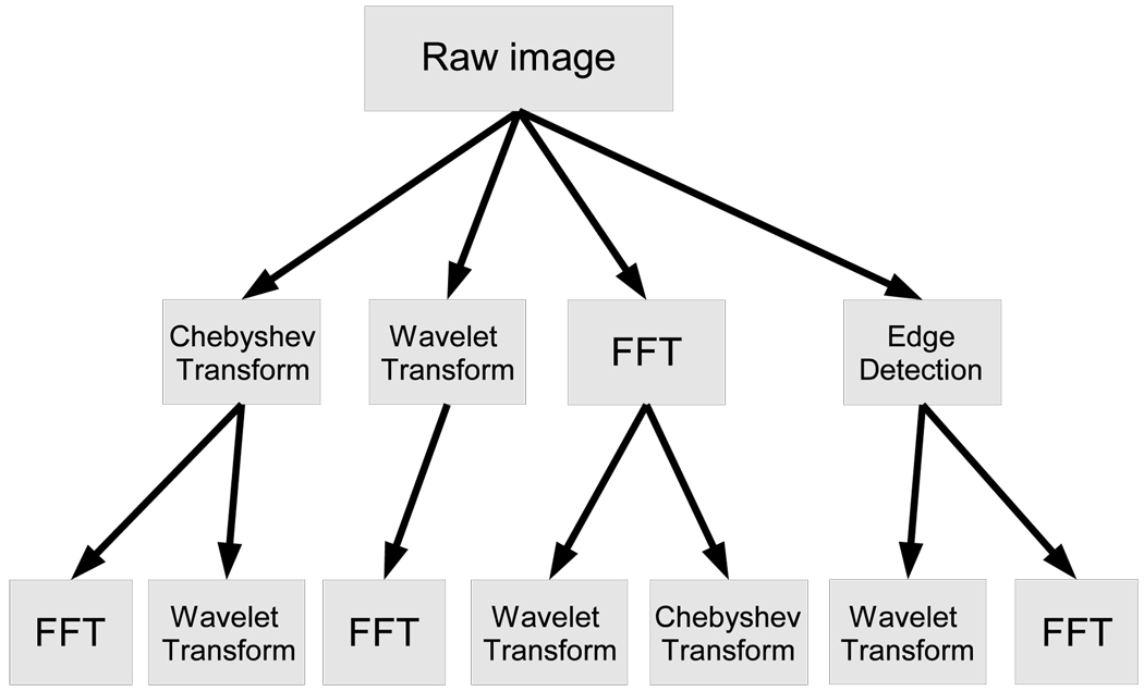
In order to extract more image descriptors, the algorithms are applied not only on the raw pixels, but also on several transforms of the image and transforms of transforms. The image transforms are FFT, Wavelet (Symlet 5, level 1) two-dimensional decomposition of the image, and Chebyshev transform. Another transform that is used is Edge Transform, which is simply the magnitude component of the Prewitt gradient. The various combinations of the compound image transforms are described in Figure 1. The entire set of image features extracted from all image transforms described in Figure 1 consists of a total of 2633 numeric image descriptors. Detailed description and source code of the image features are available at (Shamir et al., 2008b; Orlov et al., 2008).

Fig. 1.

Image transforms and paths of the compound image transforms.

While this set of image features provides a numeric description of the image content, not all image features are assumed to be equally informative, and some of these features are expected to represent noise. In order to select the most informative features while rejecting noisy features, each image feature is assigned with a simple Fisher score (Bishop, 2006), and 85% of the features (with the lowest Fisher scores) are rejected and do not affect the classification. The Fisher score can be conceptualized as the ratio of variance of class means from the pooled mean to the mean of within-class variances, and therefore reflect the discriminative power of the feature. The feature vectors can then be classified by a simple weighted nearest neighbor rule, such that the feature weights are the Fisher scores.

The data used for this study are fully extended weight bearing radiographs taken during a regularly scheduled study visit of the Baltimore Longitudinal Study of Aging (BLSA) (Shock et al., 1984). The dataset included longitudinal conventional film-screen radiographs of the knees, AP, standing, with resolution of approximately 8–10 line pairs/mm. All images were taken at a standard distance and would have had the same magnification. Although the sizes of the actual knees can be different, no attempt was made to normalize for the size in order to preserve the signal of the low-level image features. The X-ray films were digitized using a UMAX PowerLook 1100 scanner at 300 DPI, and saved as 2550×3000 16-bit (14-bit effective) lossless TIFF files. All images were then normalized to a fixed mean and standard deviation. Each knee image was independently assigned a KL grade (0–4) by two trained readers as described by Hochberg, Lethbridge-Cejku & Tobin (2004), with discordant grades adjudicated by a third reader. It is important to note that all X-rays were taken from participants in the BLSA study without any specific selection criteria, and not necessarily from people who reported pain symptoms or were diagnosed as having OA in one of their other joints. This policy provided a uniform and unbiased representation across the study population.

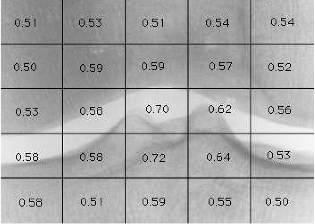
In previous work (Shamir et al., 2008a) we used WND-CHARM to diagnose existing OA. Here we use a similar approach to analyzing scanned film X-rays to detect early signs of developing OA, or predict risk of developing OA in the future. As before, the method first detects the center of the knee joint and extracts 700×500 pixels around it to form a sub-image of a centered joint. Figure 4 is an example of a 700×500 joint center image used for the computer-aided image analysis. Finding the joint in a given knee X-ray image is performed by first downscaling the image by 0.1, and then scanning the image with a 15×15 shifted window. For each position, the Euclidean distances between the 15×15 pixels of the shifted window and 20 15×15 pre-defined joint center images are computed using Equation 1,

$$d_{i,w}=\sqrt{{\displaystyle \sum _{y=1}^{15}{\displaystyle \sum _{x=1}^{15}(I_{x,y}}-W_{x,y}{)}^2}}$$ (1)

where W_x,y is the intensity of pixel x,y in the shifted window W, I_x,y is the intensity of pixel x, y in the joint image I, and d_i,w is the Euclidean distance between the joint image I and the 15×15 shifted window W.

Fig. 4.

Classification accuracy of predicting KL grade 3 using different areas of the knee joints. The strongest signal (0.72) comes from the part of the tibia just beneath the joint.

Since the proposed implementation uses 20 joint images, 20 different distances are computed for each possible position of the shifted window, but only the shortest of the 20 distances is recorded. After scanning the entire (width/10–15)×(height/10–15) possible positions, the window that recorded the smallest Euclidean distance is determined as the center of the joint, and the 700 × 500 pixels around this center form an image that is used for the automated analysis. Since each image contains exactly one joint, and since the rotational variance of the knees is fairly minimal, this simple and fast method was able to successfully find the joint center in all images in the dataset.

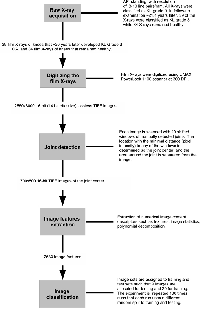
Figure 2 summarizes the entire process of the data handling, from the acquisition of the film X-rays to the image classification.

Fig. 2.

Summary of the X-ray data processing: Film X-ray acquisition, digitization of the film X-rays, automatic joint detection and separation of the joint area from the image, computing image features and then classifying each image based on the feature values.

3 Results

The computer-aided OA detection method (Shamir et al., 2008a) was used to classify two sets of X-rays. The first set contained 39 pairs of X-rays wherein the first was classified by expert radiologists as KL grade 0 (normal), and the second, obtained ~20 years later, was classified as KL grade 3 (moderate OA). The second set contained 84 pairs of knee X-rays wherein both were classified by expert radiologists as KL grade 0 (normal) at both time points. The mean difference between the date of the initial classification and the follow-up was 21.4 years, with a standard deviation of 1.35 years. The mean age of the participants in both sets was set to 52 years by removing 22 images from the set of the knees that remained healthy (originally there were 106 images). Male/female ratio in the two sets was ~0.64 and ~0.61, respectively. Table 1 summarizes the distribution of the data by KL grade.

Table 1.

The distribution of the number of images, gender ratio, mean age and mean difference between the initial and follow-up classification

	KL Grade 0	KL Grade 1	KL Grade 2	KL Grade 3
No. of images	84	51	25	39
Men/Women	0.64	0.62	0.59	0.61
Mean age (years)	52	48.7	49.5	52
Mean difference (years)	21.5	21.8	20.6	21.2

The automatic image classifier was trained using 30 images of future KL grade 3 and 30 images of future KL grade 0, and was tested using nine images from each of the two classes. The experiment was repeated 100 times, such that in each run different images of each class were randomly assigned for training and testing.

Experimental results show that the accuracy of predicting the development of moderate OA (KL 3) in a normal knee in the following ~20 years is 72% (P<0.00001), with sensitivity of 74% and specificity of 70%. In a similar experiment, the 39 future moderate OA X-rays were replaced with 25 X-rays of knees that later progressed to KL grade 2 (mild definite OA), such that 20 images were used for training, and five for testing. Experimental results show that the development of mild OA in the next ~20 years can be predicted with an accuracy of 62% (P<0.01). For KL grade 1 (doubtful OA), no prediction better than random was achieved (30 images for training, 9 images for testing). Table 2 summarizes the experimental result figures.

Table 2.

Experimental results for predicting future KL grade 1, 2 and 3. In all experiments 84 X-rays of future KL grade 0 were used. The detection accuracy figures are the mean of 100 runs such that in each run different images of each class were randomly assigned for training and testing.

KL grade	Training images per class	Test images per class	Accuracy (%)	Sensitivity (%)	Specificity (%)
1	30	9	72 (P<0.00001)	74	70
2	25	5	62 (P<0.01)	63	61
3	30	9	50	50	50

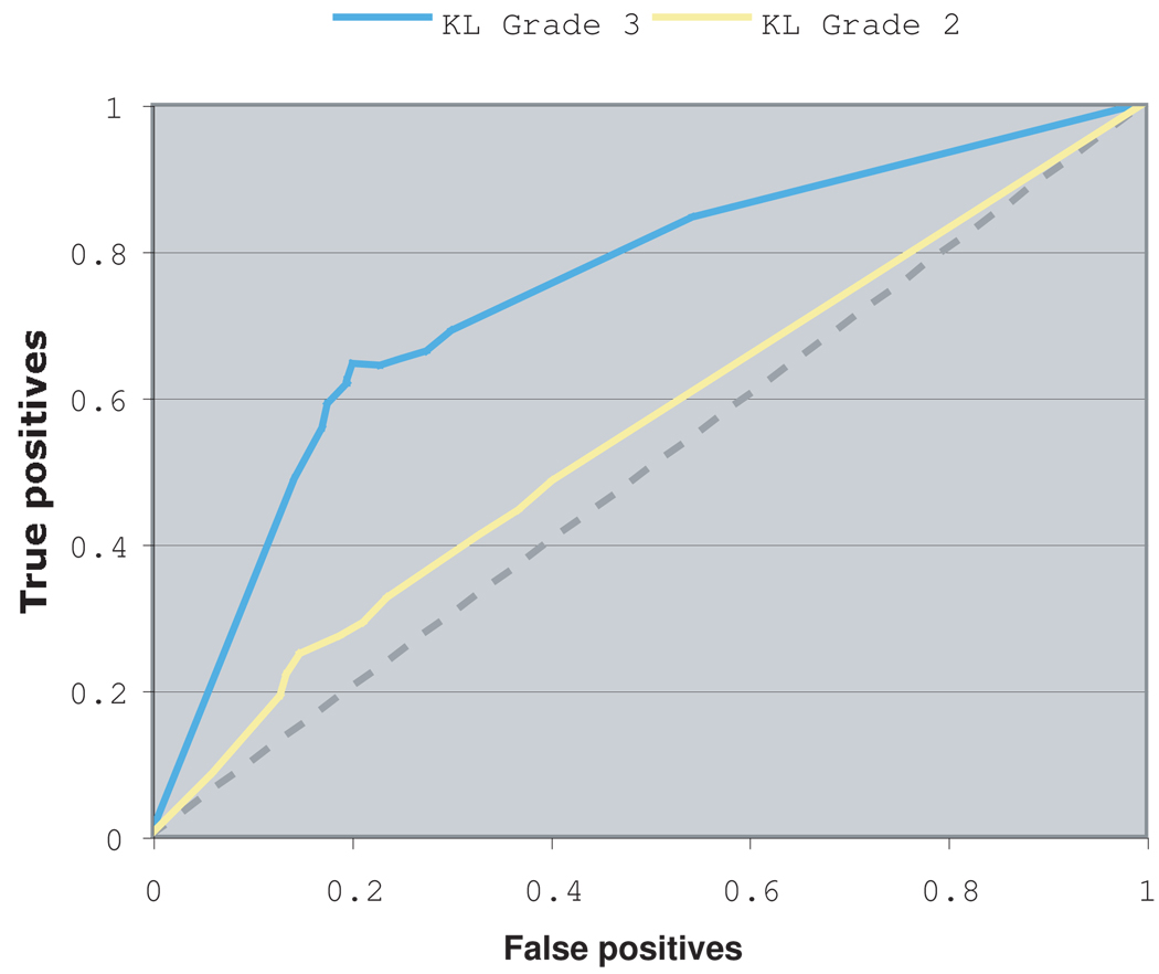
As described in Section 2, the early detection of moderate OA is determined by the system based on the similarity of a given X-ray image to known samples of KL-0 knees that later developed into KL grade 3. The raw image similarity values to each class of images are then normalized to the interval [0, 1], and represent the likelihoods of the image to belong in the different classes, as explained in (Shamir et al., 2008b). Figure 3 shows the ROC that is produced by changing the threshold similarity value for detecting a future KL-3 OA.

Fig. 3.

ROC of the prediction of KL grade 2 and 3 OA

To determine the areas of the joint that provide the strongest predictive signal for the development of moderate OA, each X-ray image was split into 25 rectangular, equal-sized tiles. This provided 25 different datasets, where each dataset consisted of all tiles at a specific location in the image. Figure 4 shows the prediction accuracy of moderate OA development in the different areas of the knee joint.

As expected, a large part of the predictive signal comes from areas containing the joint. Interestingly, a substantial and even slightly higher signal comes from a part of the tibia just beneath the joint. This shows that the structure of the tibia is not only informative for the detection of present OA (Podsiadlo, Wolski & Stachowiak, 2008; Lankester et al., 2008), but also for early detection many years before radiographic signs of OA can be noticed in the X-ray. It also shows that alterations of the bone structure associated with the early stages of OA (Bolbos et al., 2008) starts before cartilage degeneration is noticeable using plain radiography, and can be detected at a much earlier stage. Other areas of the tibia and the femur that are more distant from the joint center were also tested, but provided no predictive signal.

The P values are computed automatically by the software used for the experiments (Shamir et al., 2008b), and simply reflect the probability of a binary distribution of the two sets that is equal or better than the classification accuracy. For instance, the P value for the detection of future KL grade 3 is the probability that the set of X-rays used for that experiment (future KL grade 0 X-rays and future KL grade 3 X-rays) can be randomly divided into two sets such that 72% or more of the future KL grade 3 X-rays fall within one set, and 72% or more of the future KL grade 0 fall within the other.

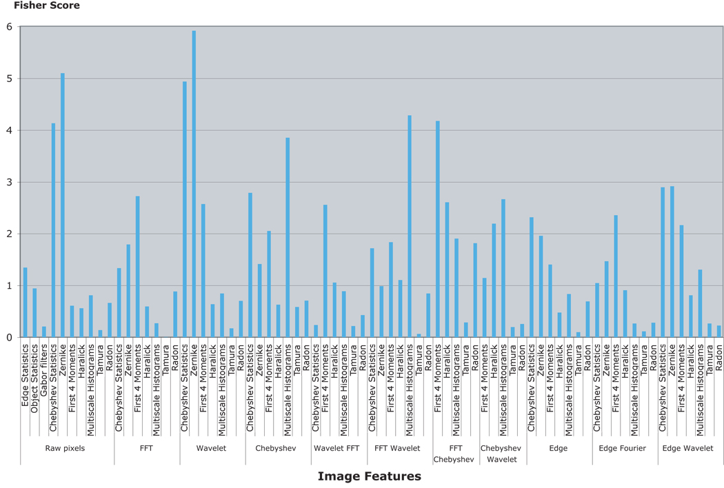
As discussed in Section 2, not all image features are expected to be equally informative. Figure 5 shows the Fisher scores (sum of the Fisher scores of all bins of a feature group) of the different features extracted from the different image transforms.

Fig. 5.

Fisher scores of the different image features. The most informative features are the features that are based on polynomial decomposition of the image and low-level statistics of the pixel intensity values.

As the graph shows, the most informative image features are computed using the image transforms, such as the Zernike features computed from the Wavelet transform and the first four moment features computer from the Fourier transform of the image. These combinations are highly non-intuitive for the human perception. Informative image features computed using the raw pixels, such as Zernike and Chebyshev statistics, are based on the polynomial decomposition of the image and are also non-intuitive to the human eye. The informativeness of these features can be used by an algorithm such as WND-CHARM, which applies a systematic search among a large set of image features for the most informative content descriptors, and is not biased by an hypothesis or by visual features that are easier to sense by the human eye.

4 Discussion

Here we showed that predictive radiographic features of OA development can be detected by computer-aided analytic methods years before radiographic OA is noticeable by the unaided eye. The prediction accuracy of 72% is certainly higher than random, and shows that radiographic evidence of OA can be detected using X-rays at the time when the joint is considered normal using the standard KL classification system. Furthermore, the results of this study suggest that the regions of knee image that contain the joint and the tibia just beneath the joint space provide the most predictive information.

We acknowledge the following study limitations. First, this study is comprised of a limited sample of images. Second, the X-rays available for use were obtained in the fully upright position with weight-bearing, and were not enhanced by use of the semi-flexed or fluoroscopically-aligned images. Third, this study focuses on radiographic OA development without regard to symptom presence or severity both of which are important clinical outcomes to include in future studies. Finally, because follow-up images were obtained during routine visits, we cannot determine when knees transitioned from normal to a higher KL grade.

As discussed in Section 3, the association between the mathematically expressed image content descriptors and their corresponding features of OA progression is not trivial, and it is difficult to link each specific image feature to its corresponding structural alteration of the joint. However, as shown by Figure 5, the most informative image content descriptors are the low-level image features such as Zernike polynomials and Chebyshev statistics, that measure small variations in the pixel values that can be difficult to sense by the unaided eye. As discussed by Boniatis et al. (2006), the low-level pixel intensity variations reflect anatomical structures in the joint (Bocchi et al., 1997), and correlate with biochemical, biomechanical and structural alterations of the articular cartilage and the subchondral bone tissues (Aigner & McKenna, 2002; MartelPelletier & Pelletier, 2003). These processes have been associated with cartilage degeneration in OA (Buckwalter & Mankin, 1997; Rodenacker & Bengtsson, 2003), and are therefore expected to affect the joint tissues in a fashion that can be sensed by the low-level texture and pixel variations of the radiograph.

Despite the aforementioned limitations, this study uniquely utilizes existing images that were routinely obtained in all willing participants at two points in time, and is therefore independent of the bias introduced by clinical indications (i.e. presence of painful symptoms). Similarly, this method of automated-image analysis is not subject to the bias inherent in clinical X-ray readings. The results imply that this data-driven analysis method can utilize radiographic images in their entirety, to detect features present in normal X-rays that are predictive of OA development and therefore could be applicable to large-scale observational studies, and evaluated for risk stratification in interventional studies.

References

- Aigner T, McKenna L. Molecular pathology and pathobiology of osteoarthritic cartilage. CMLS Cell. Mol. Life Sci. 2002;59:5–18. doi: 10.1007/s00018-002-8400-3. [DOI] [PMC free article] [PubMed] [Google Scholar]
- Bishop CM. Pattern Recognition and Machine Learning. Springer Press; 2006. [Google Scholar]
- Bocchi L, Coppini G, De Dominicis R, Valli G. Tissue characterization from X-ray images. Med. Eng. Phys. 1997;19:336–342. doi: 10.1016/s1350-4533(96)00078-1. [DOI] [PubMed] [Google Scholar]
- Bolbos RI, Zuo J, Banerjee S, Link TM, Benjamin MC, Li X, et al. Relationship between trabecular bone structure and articular cartilage morphology and relaxation times in early OA of the knee joint using parallel MRI at 3T. Osteoarthritis Cartilage. 2008;16:1150–1159. doi: 10.1016/j.joca.2008.02.018. [DOI] [PMC free article] [PubMed] [Google Scholar]
- Boniatis I, Costaridou L, Cavouras D, Kalatzis I, Panagiotopoulos E, Panayiotakis G. Osteoarthritis severity of the hip by computer-aided grading of radiographic images. Med. Bio. Eng. Comp. 2006;44:793–803. doi: 10.1007/s11517-006-0096-3. [DOI] [PubMed] [Google Scholar]
- Boniatis I, Cavouras D, Costaridou L, Kalatzis I, Panagiotopoulos E, Panayiotakis G. Computer-aided grading and quantification of hip osteoarthritis severity employing shape descriptors of radiographic hip joint space. Comp. in Bio. and Med. 2007;37:1786–1795. doi: 10.1016/j.compbiomed.2007.05.005. [DOI] [PubMed] [Google Scholar]
- Buckwalter A, Mankin HJ. Instructional course lectures, the American Academy of Orthopaedic Surgeons Articular Cartilage. Part II: degeneration and osteoarthrosis, repair, regeneration, and transplantation. Journal of Bone and Joint Surgery. 1997;79:612–632. [Google Scholar]
- Gabor D. Theory of communication”. Journal of IEEE. 1946;93:429–457. [Google Scholar]
- Gradshtein I, Ryzhik I. Table of integrals, series and products. 5 ed. Academic Press; 1994. p. 1054. [Google Scholar]
- Gray SB. Local properties of binary images in two dimensions”. IEEE Transactions on Computers. 1978;20:551–561. [Google Scholar]
- Gregorescu C, Petkov N, Kruizinga P. Comparison of texture features based on Gabor filters. IEEE Transactions on Image Processing. 2002;11:1160–1167. doi: 10.1109/TIP.2002.804262. [DOI] [PubMed] [Google Scholar]
- Hadjidementriou EM, Grossberg, Nayar S. Spatial information in multiresolution histograms; IEEE Conf. on Computer Vision and Pattern Recognition; 2001. p. 702. [Google Scholar]
- Haralick RM, Shanmugam K, Dimstein I. Textural features for image classification. IEEE Transaction on System, Man and Cybernetics. 1973;6:269–285. [Google Scholar]
- Hochberg MC, Lethbridge-Cejku M, Tobin JD. Bone mineral density and osteoarthritis: data from the Baltimore Longitudinal Study of Aging. Osteoarthritis Cartilage. 2004;12:S45–S48. doi: 10.1016/j.joca.2003.09.008. [DOI] [PubMed] [Google Scholar]
- Kellgren JH, Lawrence JS. Radiologic assessment of osteoarthritis. Ann. Rheum Dis. 1957;16:494–501. doi: 10.1136/ard.16.4.494. [DOI] [PMC free article] [PubMed] [Google Scholar]
- Kellgren JH, Jeffrey M, Ball J. Atlas of standard radiographs. Oxford: Blackwell Scientific; 1963. [Google Scholar]
- Lankester BJA, Cottam HL, Pinskerova V, Eldridge JDJ, Freeman MAR. Variation in the anatomy of the tibial plateau: a possible factor in the development of anteromedial osteoarthritis of the knee. Journal of Bone Joint Surg. 2008;90:330–333. doi: 10.1302/0301-620X.90B3.19898. [DOI] [PubMed] [Google Scholar]
- Lim JS. Two-dimensional signal and image processing. Prentice Hall; 1990. pp. 42–45. [Google Scholar]
- Lynch JA, Hawkes DJ, Buckland-Wright JC. Analysis of texture in macroradiographs of osteoarthritic knee using the fractal signature. Phys. Med. Biol. 1991;36:709–722. doi: 10.1088/0031-9155/36/6/001. [DOI] [PubMed] [Google Scholar]
- MartelPelletier J, Pelletier JP. Osteoarthritis: recent developments. Curr. Opin. Rheumatol. 2003;15:613–615. [Google Scholar]
- Messent EM, Ward RJ, Tonkin CJ, Buckland-Wright JC. Cancellous bone difference between knees with early, definite and advanced joint space loss: A comparative quantitative macroradiographic study. Osteoarthritis Cartilage. 2005;13:39–47. doi: 10.1016/j.joca.2004.10.009. [DOI] [PubMed] [Google Scholar]
- Orlov N, Shamir L, Macura T, Johnston J, Eckely DM, Goldberg I. “WND-CHARM: Multi-purpose image classification using compound image transforms,”. Pattern Recognition Letters. 2008;29:1684–1693. doi: 10.1016/j.patrec.2008.04.013. [DOI] [PMC free article] [PubMed] [Google Scholar]
- Otsu N. A threshold selection method from gray level histograms. IEEE Transactions on System, Man and Cybernetics. 1979;9:62–66. [Google Scholar]
- Podsiadlo P, Wolski M, Stachowiak GW. Automated selection of trabecular bone regions in knee radiographs. Med. Phys. 2008;35:1870–1883. doi: 10.1118/1.2905025. [DOI] [PubMed] [Google Scholar]
- Podsiadlo P, Dahl L, Englund M, Lohmander L, Stachowiak G. Differences in trabecular bone texture between knees with and without radiographic osteoarthritis detected by fractal methods. Osteoarthritis Cartilage. 2008;16:323–329. doi: 10.1016/j.joca.2007.07.010. [DOI] [PubMed] [Google Scholar]
- Prewitt JM. In: Object enhancement and extraction, Picture processing and psychopictoris. Lipkin BS, Rosenfeld A, editors. New York: Academic; 1970. pp. 75–149. [Google Scholar]
- Radin EL, Rose RM. RM, Role of subchondral bone in the initiation and progression of cartilage damage. Clin. Orthop. 1986;213:34–40. [PubMed] [Google Scholar]
- Shamir L, Ling SM, Scott WW, Bos A, Orlov N, Macura T, et al. Knee X-ray image analysis method for automated detection of Osteoarthritis. IEEE Trans. on Biomed. Eng. doi: 10.1109/TBME.2008.2006025. In Press. [DOI] [PMC free article] [PubMed] [Google Scholar]
- Shamir L, Orlov N, Macura T, Eckley DM, Johnston J, Goldberg I. Wndchrm - An Open Source Utility for Biological Image Analysis. BMC Source Code for Biology and Medicine. 2008;3:13. doi: 10.1186/1751-0473-3-13. [DOI] [PMC free article] [PubMed] [Google Scholar]
- Shamir L, Orlov N, Eckley DM, Macura T, Goldberg I. IICBU-2008 - A Benchmark Suite for Biological Imaging. Med. Bio. Eng. Comp. 2008;46:943–947. doi: 10.1007/s11517-008-0380-5. [DOI] [PMC free article] [PubMed] [Google Scholar]
- Shock NW, Greulich RC, Andres R, R, Arenberg D, Costa PT, Lakatta EG, et al. Normal human aging: the Baltimore Longitudinal Study of Aging. Washington, DC: Government Printing Office; NIH Publication No. 84–2450. 1984
- Tamura H, Mori S, Yamavaki T. Textural features corresponding to visual perception”. IEEE Transactions on System, Man and Cybernetics. 1978;8:460–472. [Google Scholar]
- Teague MR. Image analysis via the general theory of moments. Journal of the Optical Society of America. 1979;70:920–930. [Google Scholar]