Differential Effect of the State Children's Health Insurance Program Expansions by Children's Age

Abstract

Research Objective

This paper tests for differences in the effect of State Children's Health Insurance Program (SCHIP) on children's insurance coverage and physician visits across three age groups: pre-elementary school-aged children (pre-ESA), ESA children, and post-ESA children.

Data Source

The study uses two cross sections of the Survey of Income and Program Participation (SIPP) from the 1996 and 2001 panels.

Study Design

A difference-in-differences approach is used to estimate the effect of SCHIP on coverage and physician visits of newly eligible children of different age groups.

Data Collection

Demographic, insurance, and physician visit information for children in families with income below 300 percent of federal poverty line were extracted from the SIPP.

Principal Findings

Uninsurance rates for post-ESA children declined due to SCHIP while public coverage and the likelihood of visiting a physician increased. Estimates of cross-age differences show that post-ESA children experienced a larger decline in uninsurance rates compared with pre-ESA and ESA children and a larger increase in physician visits compared with ESA children.

Conclusions

The higher rate of physician visits for post-ESA children due to SCHIP demonstrates the importance of extending insurance coverage to teens as well as young children.

In 1996, a year before the State Children's Health Insurance Program (SCHIP) was signed into law, a federal mandate set different income eligibility levels for public health insurance by age. States were required to extend eligibility for public health insurance to children younger than 6 years old (henceforth pre-ESA, which stands for pre-elementary school-aged) in families with income below 133 percent of the federal poverty line (FPL), and to children 6–12 years old (henceforth ESA) in families with income under 100 percent FPL eligible, while no mandate existed for children aged 13–18 (henceforth post-ESA). The difference in eligibility levels between adolescents and younger children may suggest that policy makers before SCHIP thought that younger children needed insurance more than adolescents. The SCHIP expansion decreased the disparity in income eligibility across age groups within states by expanding income eligibility disproportionately, with a larger increase in eligibility for older children than for younger. By 2001, after every state had implemented some form of the SCHIP expansion, the income eligibility for public health insurance in almost all states was the same for all children under the age of 19. These differences in the size of the expansion led to the empirical question that this paper addresses: Did the SCHIP expansion affect newly eligible children of different ages in different ways?

It is unclear a priori which age group (pre-ESA, ESA, or post-ESA) would be most affected by the SCHIP expansion. On the one hand, pre-ESA children need more health services, implying that if a public health insurance policy becomes available for both pre-ESA and post-ESA children who cannot afford private health insurance coverage, then pre-ESA children will be more likely to take up public coverage. On the other hand, the older children's income eligibility thresholds were much lower before the SCHIP expansion, implying that the newly eligible children from the older age group come on average from families with lower incomes. Because evidence from the earlier Medicaid expansions suggests that take-up rates fall as income increases, one would expect that take-up rates would be higher for the older age group (Currie and Gruber 1996; Card and Shore Sheppard 2004;). These two countervailing factors imply that both pre-ESA and post-ESA children potentially could have been the group most affected by the SCHIP expansion.

Using Survey of Income and Program Participation (SIPP) data from 1996 and 2001, I assess the effects of SCHIP on insurance coverage and physician visits in three ways. First, using a difference-in-differences approach, I estimate the take-up rate of public health insurance coverage for each age group, which is the fraction of newly eligible children who are covered by public health insurance, and test whether take-up rates are the same across age groups. Second, I explore whether public health insurance coverage substituted for private coverage (what is known as the crowd-out effect) or whether the increase in public coverage reduced the uninsurance rate. I also test whether the declines in private coverage and uninsurance rates are significantly different across age groups. Third, I estimate whether SCHIP affected the percentage of children seeking treatment, which I measure using the percentage of children visiting a physician at least once in the last 12 months before the SIPP interview, testing whether the increase in physician visits differs across age groups.

The effect of SCHIP expansion on coverage has been addressed before (Rosenbach et al. 2001; Zuckerman et al. 2001; Cunningham, Hadley, and Reschovsky 2002; Cunningham, Reschovsky, and Hadley 2002; Lo Sasso and Buchmueller 2004; Hudson, Selden, and Banthin 2005; Bansak and Raphael 2006; Buchmueller, Lo Sasso, and Wong 2007; Gruber and Simon 2007). These studies find take-up rates ranging from 5 to 18 percent, depending on the specification and data used. However, the studies do not explore differences in the effect of SCHIP across age or income levels. Literature examining earlier Medicaid expansions (Currie and Gruber 1996; Card and Shore Sheppard 2004;) does address whether the expansions had a different effect on coverage at different income levels. However, the earlier Medicaid expansion applies to pre-ESA and ESA children at lower income levels, which may not be valid for the SCHIP expansion.

Although the SIPP was used to estimate the effect of prior Medicaid expansions (see, e.g., Blumberg, Dubay, and Norton 2000; Ham and Shore-Sheppard 2005;), this study is the first to use the SIPP to estimate the effect of the SCHIP. Using the SIPP provides a better measure of health insurance than does the more commonly used Current Population Survey (CPS) (Short 2001). The study also provides the first test of whether a public health insurance program expansion has different impacts across different populations. Unlike most earlier studies of Medicaid or SCHIP expansions, this paper combines the effect of a health care expansion on coverage with an important indicator of health care treatment: physician visits.

This paper is organized as follows: the second section explains the methods used to test and assess the effects of SCHIP on health insurance coverage and physician visits; the third section describes the data used; the fourth section reports trends over time in health insurance coverage as well as physician visits and regression results; and the fifth section concludes.

METHODS

The main difficulty in assessing the effect of SCHIP is finding an appropriate treatment group consisting of individuals affected by SCHIP and a control group consisting of individuals with characteristics similar to the treatment group unaffected by SCHIP. Because individuals are not assigned to treatment and control groups randomly, and this classification is not present in the data, I simulate income eligibility for public health insurance based on rules that existed pre- and post-SCHIP for two cross sections of the 1996 and 2001 SIPP. The simulation of income eligibility for public health insurance coverage is based on a child's age and family income, as well as the income eligibility standards in the child's state of residence (an appendix detailing the simulation is available upon request from the author). Hence, the sample can be divided into three groups: children who are income eligible for public health insurance under both the 1996 and 2001 rules, children who are income eligible under the 2001 rules but not under the 1996 rules, and children who are not income eligible under either the 1996 or the 2001 rules.

The newly eligible children in 2001 represent a group that should have been affected by SCHIP and are considered the treatment group. Hence, the difference in health insurance coverage and physician visits for the treatment group between 1996 and 2001 measures changes in these outcomes pre- and postexpansion. However, because other economic factors could affect the changes in outcomes observed between 1996 and 2001, I would like to have a group that was not affected by the SCHIP expansion, but was affected by the economic trends of the period and at the same time have similar characteristics as the treatment group. It is difficult to identify a group of children unaffected by the SCHIP expansion at all that also has similar characteristics to the treatment group. On the one hand, children who were eligible for public coverage before the SCHIP expansion could have taken up public coverage after the expansion as a result of the aggressive advertisement for the program. On the other hand, children at higher income levels who are not eligible for SCHIP tend to have very different demographic characteristics. For the base specification, I use the not newly eligible children (including always eligible and never eligible children) from families with income below 300 percent FPL to be the control group because they are close to the treatment group in income and they should only be marginally affected by the SCHIP expansion. Using children above 300 percent of FPL would have contaminated the control group with children that have very different characteristics than the treatment group. Using the change in outcome for the newly eligible minus the change in outcome for the not newly eligible provides me with a difference-in-differences estimator.

I recognize that my treatment group is not ideal because children in the control group who are eligible based on eligibility rules in 1996 (and 2001) may also be affected by SCHIP and because the eligibility simulation may have misassigned newly eligible children to the control group. But, at the very least, the comparison group approach I use identifies whether the observed effects of SCHIP on health insurance and at least one physician visit is age group specific, and whether the effects are primarily found for the newly eligible children of 2001—the treatment group.

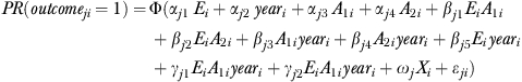
I use the following pooled, weighted difference-in-differences probit model to estimate the effect of SCHIP on the newly eligible children of the three age groups:

(1)

where dependent variable outcome_ji is a dummy variable equal to 1 if the child has health insurance coverage of type j (public, private, uninsured) or visited a physician in the last 12 months. The variable E_i is a dummy variable equal to 1 if the child is eligible for public health insurance under 2001 income eligibility rules but not under 1996 rules. The year dummy equals 1 if the sample year is 2001 and 0 otherwise. The variables A_1i and A_2i are dummy variables that are equal to 1 if the child is ESA and post-ESA, respectively. The vector X_i contains demographic characteristics, including the child's gender, race/ethnicity (white, Hispanic, black, and other), age dummies, number of individuals in the household, number of children younger than 6, type of household (both parents present, mother only, and father only), number of workers in the household, highest education attainment of the parents (no high school education, some high school education, high school graduate, some college education, associate degree, college degree, and advanced degree), and urban residence indicator. I include state dummies and state unemployment rates to capture differences in economic conditions across states. Standard errors are clustered by state to account for possible serial correlation of the outcome at the state level.

The coefficient β_j5 and the sum of the coefficients β_j5+γ_1j and β_j5+γ_2j represent the difference-in-differences estimate of the effect of SCHIP on the outcome for pre-ESA, ESA, and post-ESA children, respectively. In order to asses the size of the effect SCHIP has on an outcome, I will report the average marginal effect (AME) of the coefficients β_j5, β_j5+γ_1j, and β_j5+γ_2j (Bartus 2005). The differential effects of the outcome across age groups are tested using the following t-tests: γ_1j=0 for the difference between pre-ESA and ESA; γ_2j=0 for the difference between pre-ESA and post-ESA; and γ_2j−γ_1j=0 for the difference between post-ESA and pre-ESA.

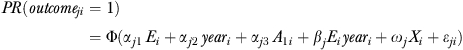
For comparison, in order to estimate the effect for all children, I use a similar probit model that excludes the age-groups interaction terms.

(2)

In this model the coefficient β_j is the all children difference-in-differences estimator of the effect of SCHIP (alternative methods and their results are available upon request from the author).

DATA

This study focuses on the health insurance and physician visit trends exhibited in the SIPP. The purpose of SIPP is to provide information about the income and program participation of individuals and households. The SIPP is a longitudinal survey that randomly selects a nationally representative sample of households in the civilian noninstitutional U.S. population, tracking individuals in those households over time. The average SIPP response rate for the first wave is 92.3 percent; however, subsequent waves suffer from attrition. SIPP respondents report whether they were covered by specific sources of public or private health insurance on a monthly basis (Medicare, Medicaid, SCHIP, other public, employment-based private, and other private). Individuals are considered publicly (privately) covered if they answered “yes” to any of the public (private) coverage questions. Individuals who are not privately or publicly covered are considered uninsured. Information on physician visits is obtained only in the third, sixth, ninth, and twelfth waves in the 1996 SIPP, and in the third, sixth, and ninth waves in the 2001 SIPP (U.S. Census Bureau 2001).

To limit the attrition rate and have comparable pre- and post-SCHIP expansion data, I draw on data from the third waves of the 1996 and the 2001 SIPP panels, which correspond to the September–December 1996 and 2001 responses to the survey, respectively, and serve as analogous pre- and post-SCHIP samples. I further limit the sample to children in families with income below the 300 percent of FPL.

There are several noteworthy advantages to using the SIPP over the more commonly used CPS. First, the health insurance variables in the SIPP are measured on a monthly basis, compared with the CPS, which measures health insurance on an annual basis. Hence, the SIPP is generally considered more precise (Short 2001). Furthermore, the third wave of the SIPP provides yearly physician visit information, which cannot be obtained from the CPS. The presence of any doctor visits represents a key indicator of access to care and has been shown to be indicative of improvements in health status, regardless of income level (Shi and Starfield 2001).

RESULTS

As explained earlier, to evaluate the effect of SCHIP on a target population, I divide the sample of children in families with income below the 300 percent FPL into two groups: “newly eligible” and “not newly eligible.”Table 1 shows weighted sample statistics of key socioeconomic variables for children in three age groups—pre-ESA, ESA, and post-ESA—by their newly eligible status in families with income below 300 percent FPL.1 The sample contained a total of 29,591 children from 45 states and the District of Columbia.2 The control and treatment groups have similar family size and number of children under 6 years old in the household. The unemployment rate, gender, and the race/ethnicity profiles of the treatment and controls groups seem comparable. However, children from the treatment groups have parents with higher education attainment and are more likely to be employed.

Table 1.

Descriptive Statistics of Key Variables for Children in Families with Income <300 Percent FPL

	Ages 0–5		Ages 6–12		Ages 13–18
Variable	Not Newly Eligible	Newly Eligible	Not Newly Eligible	Newly Eligible	Not Newly Eligible	Newly Eligible
Number of children under 6 in household	1.871	1.798	0.896	0.796	0.327	0.356
Unemployment rate	0.051	0.051	0.051	0.052	0.051	0.051
	(0.009)	(0.010)	(0.010)	(0.010)	(0.009)	(0.010)
Number of persons in the household	4.378	4.516	4.593	4.713	4.318	4.535
	(1.649)	(1.691)	(1.766)	(1.730)	(1.754)	(1.780)
Gender of child
Male	0.511	0.519	0.517	0.525	0.524	0.511
Female	0.489	0.481	0.483	0.475	0.476	0.489
Race/ethnicity
White	0.524	0.585	0.536	0.561	0.596	0.497
Black	0.201	0.146	0.211	0.166	0.174	0.229
Hispanic	0.230	0.216	0.202	0.224	0.174	0.219
Other	0.044	0.054	0.050	0.048	0.056	0.055
Workers in household
0 worker in household	0.233	0.061	0.264	0.065	0.264	0.141
1 workers in household	0.522	0.547	0.490	0.557	0.401	0.551
2+ workers in household	0.245	0.392	0.246	0.378	0.334	0.308
Highest education level by parents
No high school education	0.065	0.039	0.081	0.057	0.084	0.096
Some high school education	0.153	0.088	0.142	0.087	0.117	0.137
High school graduate	0.328	0.311	0.321	0.344	0.314	0.334
Some college	0.189	0.214	0.183	0.211	0.184	0.190
Associate degree	0.123	0.159	0.133	0.147	0.152	0.127
College graduate	0.099	0.131	0.100	0.109	0.104	0.081
Sample size	7,436	2,281	7,162	4,450	3,619	4,643

Notes. Computations are from the third wave of 1996 and 2001 SIPP panels; standard deviations of continuous variables are in parentheses. Observations are weighted using SIPP individual weight.

FPL, federal poverty line; SIPP, Survey of Income and Program Participation.

Table 2 shows the SIPP weighted average of health insurance coverage and doctor visits by eligibility status for each age group in four panels. The table also shows the difference in coverage (and doctor visits) between 2001 and 1996, and the unadjusted difference-in-differences estimator. The first panel of the table displays the effect of SCHIP on public health insurance coverage. Although newly eligible children of all age groups increased public coverage between 1996 and 2001, the unadjusted difference-in-differences is larger for older children (9.2 percentage points) than it is for the two younger groups (5.6 and 2.8 percentage points for pre-ESA and ESA children, respectively). The average take-up overall of 6.1 percent is at the lower end of findings in the literature. Based on my income-eligibility simulation, the newly eligible children under 300 percent of FPL represent 18 million children in 2001, which is similar to the 17.8 million children found by Dubay, Kenney, and Haley (2002) for the year 2000. Thus, the 6.1 percent estimated take-up rate implies that roughly 1.1 million children gained public coverage. The change in private health insurance coverage (second panel) shows that the two younger groups' private coverage declined more than it did for the older group (about 10.2 and 4.5 percentage points for the two younger groups, respectively, compared with 2.2 percentage points for the older group). The third panel shows the unadjusted difference-in-differences measure of the change in uninsurance rates. The newly eligible uninsurance rates declined by almost 5 percentage points for post-ESA children, whereas for pre-ESA and ESA children, the uninsurance rate increased (which is the wrong sign). The increase in uninsurance rate demonstrates the importance of controlling for other factors that could adversely affect newly eligible children in post-SCHIP period relative to pre-SCHIP. For example, since 2001 is considered a recession year while 1996 is an expansion, if a recession has a larger adverse uninsured effect on newly eligible children, then the result of the unadjusted difference-in-differences will be increasing uninsurance rates.

Table 2.

Health Insurance Coverage and Doctor Visits by Eligibility Status for Children in Families with Income <300 Percent FPL

		Newly Eligible			Not Newly Eligible
Insurance/ Doctor Visits	Age Group	1996	2001	Difference	1996	2001	Difference	DD
Public	Ages 0–5	0.175	0.257	0.082	0.410	0.437	0.027	0.056
	Ages 6–12	0.168	0.234	0.067	0.339	0.377	0.038	0.028
	Ages 13–18	0.198	0.321	0.122	0.245	0.275	0.030	0.092
	Overall	0.181	0.274	0.093	0.350	0.381	0.032	0.061
Private	Ages 0–5	0.686	0.607	−0.079	0.454	0.477	0.022	−0.102
	Ages 6–12	0.659	0.602	−0.057	0.499	0.487	−0.012	−0.045
	Ages 13–18	0.565	0.517	−0.048	0.618	0.593	−0.026	−0.022
	Overall	0.627	0.568	−0.059	0.505	0.504	−0.001	−0.058
Uninsured	Ages 0–5	0.170	0.192	0.023	0.183	0.171	−0.011	0.034
	Ages 6–12	0.209	0.228	0.019	0.202	0.202	0.000	0.019
	Ages 13–18	0.263	0.215	−0.048	0.174	0.175	0.001	−0.050
	Overall	0.222	0.216	−0.007	0.188	0.184	−0.004	−0.003
Doctor visits	Ages 0–5	0.740	0.697	−0.042	0.731	0.667	−0.064	0.022
	Ages 6–12	0.581	0.563	−0.018	0.582	0.584	0.001	−0.019
	Ages 13–18	0.571	0.618	0.047	0.617	0.589	−0.029	0.076
	Overall	0.611	0.612	0.001	0.652	0.618	−0.033	0.034
Sample size	Ages 0–5	1,295	986		4,312	3,124
	Ages 6–12	2,521	1,929		4,153	3,009
	Ages 13–18	2,571	2,072		2,112	1,507
	Overall	6,387	4,987		10,577	7,640

Notes. Computations are from the third wave of 1996 and 2001 SIPP panels. Observations are weighted using SIPP individual weight.

DD, unadjusted differences-in-differences estimator; FPL, federal poverty line; SIPP, Survey of Income and Program Participation.

The fourth panel reports changes in the probability of having at least one physician visit in the last 12 months. The unadjusted difference-in-differences measure of physician visits suggests an increase of about 2 percentage points for pre-ESA children, a decline of 2 percentage points for ESA children, and a dramatic increase in physician visits of 7.6 percentage points for post-ESA children.

The trends in health insurance coverage and physician visits depicted in Table 2 imply that the take-up of public health insurance coverage among newly eligible post-ESA children was larger than that of the other two groups. Furthermore, Table 2 also suggests that the increase in public coverage among the post-ESA group is due more to uninsured children becoming eligible and taking-up public coverage than it is due to families switching from private to public coverage after becoming eligible relative to the other two younger groups. This is apparent in both the smaller decline in private coverage and the larger decline in uninsurance rates for post-ESA children. Table 2 also provides some insight into the effect that SCHIP has on medical treatment. The increase in public health insurance or the decline in uninsurance rates for newly eligible post-ESA children translated to more children visiting a physician, something that cannot be said for ESA group.

Table 3 presents results from the pooled probit model of the effect of SCHIP on health insurance coverage and physician visits for children who are newly eligible. The first four columns show results of the AME based on the difference-in-differences method and the last three show the p-value for the tests of the differences between age groups.

Table 3.

Difference-in-Differences Estimation Results of the Average Marginal Effects and Cross-Age Group Differences Tests for Newly Eligible Children

	Average Marginal Effect Results				p-Values for Cross-Age Differences
	Ages 0–5	Ages 6–12	Ages 13–18	All Children	Ages 13–18 versus Ages 0–5	Ages 13–18 versus Ages 6–12	Ages 0–5 versus Ages 6–12
Panel A: Base specification—control group: not newly eligible children in families with income <300% FPL
Public insurance	0.055*	0.029	0.072**	0.055***	.691	.178	.262
Private insurance	−0.068**	−0.023	0.005	−0.030**	.094	.330	.181
Uninsured	0.017	0.009	−0.045***	−0.013	.001	.002	.673
At least one physician visit	0.035	−0.009	0.080***	0.045***	.299	.003	.235
Crowd-out 1: private/public	1.245	0.807	−0.066	0.538***
Crowd-out 2: 1−uninsured/public	1.317	1.303	0.380	0.757***
Panel B: Base specification with an additional state and year interaction—control group: not newly eligible children in families with income <300% FPL
Public insurance	0.057**	0.030	0.052*	0.051***	.905	.444	.224
Uninsured	0.016	0.009	−0.037***	−0.011	.006	.007	.743
At least one physician visit	0.032	−0.010	0.074***	0.044***	.305	.004	.248
Panel C: Base specification—control group: all not newly eligible children
Public insurance	0.032	0.015	0.045**	0.035***	.699	.168	.321
Uninsured	0.005	−0.006	−0.041***	−0.020***	.000	.007	.395
At least one physician visit	0.035	−0.014	0.039**	0.029***	.915	.050	.091
Panel D: Base specification—control group: never eligible children above 300% FPL as the control
Public insurance	0.001	−0.006	0.019	0.006	.559	.213	.773
Uninsured	−0.013	−0.039***	−0.044***	−0.035***	.034	.701	.048
At least one physician visit	0.046**	−0.026	0.021	0.016	.429	.130	.011

Notes. The first four columns show results of the average marginal effect based on difference-in-differences probit regressions using the third wave of both the 1996 and the 2001 SIPP panels. The last three columns present the p-value results of t-test of the differences between the affect of SCHIP on one age group relative to another based on same difference-in-differences probit regressions. All regressions control for the full interaction of newly eligible dummy, year dummy, and two dummies for ESA children and post-ESA children. The regression also controls for unemployment rate, number of persons in household, race family type (two parents, father only, mother only), child's gender, number of workers in household, number of children under 6, education of parents, MSA residence, age dummies, state dummies. Standard errors are clustered by state of residence and are calculated using the delta method.

^*p<.1 and >.05.

^**p<.5 and >.01.

^***p<.01.

ESA, elementary school aged; FPL, federal poverty line; SCHIP, State Children's Health Insurance Program; SIPP, Survey of Income and Program Participation.

In panel A, the control group is not newly eligible children in families with income <300 percent FPL. The first row of panel A reports the results for the take-up rate of public health insurance for pre-ESA, ESA, post-ESA, and all children of the base specification that uses not newly eligible children under 300 percent of FPL as the control group. The take-up results indicate that eligibility expansion for pre-ESA, post-ESA, and all children is associated with a somewhat small but statistically significant or marginally significant increase in public health insurance coverage (about 5.5 percentage points for pre-ESA children, 7.2 percentage points for post-ESA children, and 5.5 percentage points for all children). These results are similar to what has been found in the literature (although at the lower end) and correspond well to the base specification in Lo Sasso and Buchmueller (2004). The 5.5 percentage point take-up overall translates to roughly 1 million newly eligible children with public insurance (out of 18 million newly eligible children). The next row provides estimates of the effect of “new eligibility” for public health insurance on private insurance coverage. The newly eligible pre-ESA children experienced a statistically significant decline of 6.8 percentage points in private coverage, similar but somewhat larger than the increase in public coverage for the same age group. The effect of the expansion on private health insurance coverage for the other age groups of newly eligible children is small and insignificant. The small and insignificant change in private coverage for the newly eligible older group suggests that public coverage did not replace private coverage at all, and crowd-out is virtually zero.

The third row of the first panel of Table 3 shows results for the effect of the SCHIP expansion on the uninsurance rate. The results for all children are not significantly different from zero. The newly eligible post-ESA children's uninsurance rate declined by 4.5 percentage points, while I find no effect of the expansion on the uninsurance rate for newly eligible children from the two younger age groups.

The fourth row of the first panel of Table 3 shows results for the effect of the SCHIP expansion on physician visits. For the newly eligible post-ESA children and all children, the probability of visiting a physician in the last 12 months increased almost as much as the increase in public coverage (8 percentage points for the older group, and 4.5 percentage points for all children), and it is statistically significant. For newly eligible pre-ESA and ESA children, the change in the probability of them visiting a physician is not significant.

Finally, the all children specification suggests a crowd-out rate between 54 and 76 percent. The changes in public coverage and uninsurance rate for post-ESA children suggest a crowd-out rate of about 40 percent, while basing crowd-out on private and public coverage suggests a crowd-out of less than zero. Crowd-out estimates for the two younger age groups range from 80 to 130 percent for ESA children and 120 to 130 percent for pre-ESA children. The large crowd-out rates for the two younger age groups are due to the very small effect of SCHIP on the uninsurance rate. Although the point estimates of the crowd-out rates of the post-ESA group are smaller than the other two groups, the statistical test for differences from zero fails because of the large standard errors. The large standard errors around the point estimates of crowd-out also hinder any conclusion regarding differences in crowd-out across age groups.

The last three columns of Table 3 reports p-values from tests of differences in the effect of SCHIP for each outcome across age groups. The tests suggest that SCHIP had a different effect on outcomes across age groups. For the older group, although the increase in public coverage is larger than for ESA children, the t-test is not significant, which implies that higher take-up is only suggestive. The changes in the probability of visiting a physician and uninsurance rates were significantly larger for post-ESA children than for ESA children, suggesting a very different effect of SCHIP on the older group from that on ESA children. I do not find differences in public insurance take-up and physician visits between the newly eligible post-ESA children relative to pre-ESA children. However, the decline in the uninsurance rate is significantly larger for the older group.

In panel B, I use a similar control group as in panel A but include state–year interaction, and in panel C the regression specification is the same as in panel A but the control group includes all not newly eligible children (including those with income above 300 percent FPL). The results presented are consistent with the base specification. The increase in take-up is significant for the older group, which also experienced a decline in the uninsurance rate and increase in physician visits. The t-test results for panels B and C are similar to those for panel A.

In panel D, I use only children above 300 percent FPL who are not eligible for SCHIP as a control group. As noted above, the control group used previously may have been affected by the policy to a lesser extent. In this approach the control group is less likely to be affected by the policy. However, it is not optimal, because the control group has very different characteristics than the treatment group that could bias the results. The point estimate of this specification is different from the base specification showing unreliable small take-up effects of the expansion. However, similar to the base specification, the increase in take-up among post-ESA children is higher than ESA children, the uninsurance rate for post-ESA declined, and physician visits increased.

The regression results of Table 3 suggest that SCHIP had different effects on newly eligible children of different age groups. The younger group (pre-ESA) replaced private coverage with public coverage. The oldest newly eligible age group took up public coverage to become insured and to increase their use of health care services. Newly eligible ESA children seem not to have been affected by the SCHIP expansion.

One contributing factor to the differences in the probability of physician visits across age groups could be the differences across ages in the need for health care treatment. The American Academy of Pediatrics (AAP) recommends more frequent preventive care visits for children in their teens, preschool children, and infants relative to children 6–10 years old (AAP Committee on Practice and Ambulatory Medicine 2000). The results show that SCHIP affected physician visits of post-ESA, which correspond well to the level of health care needs for that group.

CONCLUSIONS

This paper tests whether the effects of the SCHIP expansion on health insurance coverage and physician visits are similar across age groups of children of low-income families. Several key differences emerge from the tests conducted. Similar to the prior literature, I find a small and marginally significant effect of SCHIP on the take-up of public coverage. However, only newly eligible pre-ESA children and post-ESA children had a small but significant increase in public health insurance coverage (approximately 5.5 and 7.2 percent, respectively, in the base specification), whereas ESA children did not. Second, I find that the increase in public coverage for newly eligible pre-ESA children did not decrease uninsurance rates significantly for this group. On the other hand, the uninsurance rates of newly eligible post-ESA children significantly declined. The differences in uninsurance rates for pre- and post-ESA children may suggest a differential effect of SCHIP. This result is fairly robust to alternative specifications.

The relative success of the SCHIP expansion on health insurance coverage is concentrated among post-ESA children, who experienced a decline in uninsurance rates of 4.5 percentage points. Children of other ages did not experience a decrease in uninsurance rates due to SCHIP. To some degree, the changes in health insurance coverage for the three age groups support findings from the earlier Medicaid expansion literature suggesting that take-up drops with income. However, pre-ESA children, who had higher income eligibility limits before SCHIP relative to ESA children, seem to have experienced an increase in take-up (although the results are not significant), which contradicts the earlier evidence from the Medicaid expansion.

Finally, the results imply an increase in physician visits for post-ESA children. In many ways, this is a more appropriate goal than increasing health insurance coverage, and a more important measure of expansion success. Although interesting, the changes in public, private, and overall coverage in themselves do not provide a measure that is related to adequacy of care. Moreover, measuring the effects of SCHIP or the success of SCHIP using one indicator for all children regardless of age seems inappropriate. It seems that there are vastly different effects of SCHIP on health insurance coverage and physician visits across age groups. Although the policy debate sometimes tends to focus on the insurance and health care needs of younger children, extending coverage to uninsured teens should also have a high priority. As this study shows, extending coverage to post-ESA children has increased the likelihood they will visit a doctor at least once a year, which provides doctors with an opportunity to counsel teens on risky behaviors, birth control, healthy eating, exercise, and to check if their immunization schedule is up to date.

Supporting Information

Additional supporting information may be found in the online version of this article:

Appendix SA1: Author Matrix.

Please note: Wiley-Blackwell is not responsible for the content or functionality of any supporting materials supplied by the authors. Any queries (other than missing material) should be directed to the corresponding author for the article.

REFERENCES

- American Academy of Pediatrics (AAP) Committee on Practice and Ambulatory Medicine. Recommendations for Preventive Pediatric Health Care. Pediatrics. 2000;105:645–6. [Google Scholar]
- Bansak C, Raphael S. The Effects of State Policy Design Features on Take-Up and Crowd-Out Rates for the State Children's Health Insurance Program. Journal of Policy Analysis and Management. 2006;26(1):149–75. doi: 10.1002/pam.20231. [DOI] [PubMed] [Google Scholar]
- Bartus T. Estimation of Marginal Effects Using Margeff. Stata Journal. 2005;5:309–29. [Google Scholar]
- Blumberg LJ, Dubay L, Norton SA. Did the Medicaid Expansions for Children Displace Private Insurance? An Analysis Using the SIPP. Journal of Health Economics. 2000;19(1):33–60. doi: 10.1016/s0167-6296(99)00020-x. [DOI] [PubMed] [Google Scholar]
- Buchmueller TC, Lo Sasso AT, Wong K. How Did SCHIP Affect the Insurance Coverage of Immigrant Children? The B.E. Journal of Economic Analysis & Policy. 2008;8(2) [Google Scholar]
- Card D, Shore Sheppard LD. Using Discontinuous Eligibility Rules to Identify the Effects of the Federal Medicaid Expansions on Low-Income Children. Review of Economics and Statistics. 2004;86(3):752–66. [Google Scholar]
- Cunningham PJ, Hadley J, Reschovsky J. The Effects of SCHIP on Children's Health Insurance Coverage: Early Evidence from the Community Tracking Study. Medical Care Research and Review. 2002;59(4):359–83. doi: 10.1177/107755802237807. [DOI] [PubMed] [Google Scholar]
- Cunningham PJ, Reschovsky JD, Hadley J. SCHIP, Medicaid Expansions Lead to Shifts in Children's Coverage. Center for Studying Health System Change Issue Brief No. 59, pp. 1–6. [PubMed]
- Currie J, Gruber J. Health Insurance Eligibility, Utilization of Medical Care, and Child Health. Quarterly Journal of Economics. 1996;111(2):431–66. [Google Scholar]
- Dubay L, Kenney G, Haley J. Children's Participation in Medicaid and SCHIP: Early in the SCHIP Era. Assessing the New Federalism Policy Brief Series No. B(B-40). Washington, DC: The Urban Institute.
- Gruber J, Simon K. Crowd-Out Ten Years Later: Have Recent Public Insurance Expansions Crowded Out Private Health Insurance? Working Paper No. 12858. Cambridge, MA: National Bureau of Economic Research. [DOI] [PubMed]
- Ham JC, Shore-Sheppard L. The Effect of Medicaid Expansions for Low-Income Children on Medicaid Participation and Private Insurance Coverage: Evidence from the SIPP. Journal of Public Economics. 2005;89(1):57–83. [Google Scholar]
- Hudson JL, Selden TM, Banthin JS. The Impact of SCHIP on Insurance Coverage of Children. Inquiry. 2005;42(3):232–54. doi: 10.5034/inquiryjrnl_42.3.232. [DOI] [PubMed] [Google Scholar]
- Lo Sasso AT, Buchmueller TC. The Effect of the State Children's Health Insurance Program on Health Insurance Coverage. Journal of Health Economics. 2004;23(5):1059–82. doi: 10.1016/j.jhealeco.2004.03.006. [DOI] [PubMed] [Google Scholar]
- Rosenbach M, Ellwood M, Czajka J, Irvin C, Coupé W, Quinn B. Implementation of the State Children's Health Insurance Program: Momentum Is Increasing after a Modest Start. Cambridge, MA: Mathematica Policy Research Inc; 2001. [Google Scholar]
- Shi L, Starfield B. The Effect of Primary Care Physician Supply and Income Inequality on Mortality among Blacks and Whites in US Metropolitan Areas. American Journal of Public Health. 2001;91(8):1246–50. doi: 10.2105/ajph.91.8.1246. [DOI] [PMC free article] [PubMed] [Google Scholar]
- Short PF. Counting and Characterizing the Uninsured. Working Paper Series. Ann Arbor, MI: Economic Research Initiative on the Uninsured.
- U.S. Census Bureau. Survey of Income and Program Participation Users' Guide. 3d Edition. Washington, DC: U.S. Census Bureau; 2001. [Google Scholar]
- Zuckerman S, Kenney GM, Dubay L, Haley J, Holahan J. Shifting Health Insurance Coverage, 1997–1999. Health Affairs. 2001;20(1):169–77. doi: 10.1377/hlthaff.20.1.169. [DOI] [PubMed] [Google Scholar]
Associated Data
This section collects any data citations, data availability statements, or supplementary materials included in this article.