Molecular Dynamics Simulations of the Dynamic and Energetic Properties of Alkali and Halide Ions Using Water-Model-Specific Ion Parameters

Abstract

The dynamic and energetic properties of the alkali and halide ions were calculated using molecular dynamics (MD) and free energy simulations with various different water and ion force fields including our recently developed water-model-specific ion parameters. The properties calculated were activity coefficients, diffusion coefficients, residence times of atomic pairs, association constants, and solubility. Through calculation of these properties, we can assess the validity and range of applicability of the simple pair potential models and better understand their limitations. Due to extreme computational demands, the activity coefficients were only calculated for a subset of the models. The results qualitatively agree with experiment. Calculated diffusion coefficients and residence times between cation−anion, water−cation, and water−anion showed differences depending on the choice of water and ion force field used. The calculated solubilities of the alkali−halide salts were generally lower than the true solubility of the salts. However, for both the TIP4P_EW and SPC/E water-model-specific ion parameters, solubility was reasonably well-reproduced. Finally, the correlations among the various properties led to the following conclusions: (1) The reliability of the ion force fields is significantly affected by the specific choice of water model. (2) Ion−ion interactions are very important to accurately simulate the properties, especially solubility. (3) The SPC/E and TIP4P_EW water-model-specific ion force fields are preferred for simulation in high salt environments compared to the other ion force fields.

Introduction

Salts of monovalent ions are highly soluble in aqueous solution, and the solvated ions have important functional roles in screening charge, moving charge, and also influencing the structure and dynamics of biomolecules such as proteins and nucleic acids.¹⁻⁷ Given this, accurate modeling of biomolecular structure, dynamics, and function requires some representative model of ionic interactions and mobile ions. In this work, we focus on the most common molecular mechanical models, specifically those based on a pairwise additive potential that includes a Coulombic treatment of the electrostatic interactions and a Lennard-Jones representation of dispersion−attraction and core repulsion. In this formulation, the potential energy (U_ij) between any pair of nonbonded atoms (i and j) in a system composed of the ions and water molecules is usually expressed as

Here, q_i and q_j are the point charges of the atoms, r_ij is the distance between atoms, and R_min,ij and ε_ij are the van der Waals radius and well depth of the Lennard-Jones potential. To represent the water, simplified point charge models such as TIP3P,(8) SPC/E,(9) and TIP4P_EW(10) are utilized. Although the models are simple, determination of the Lennard-Jones parameters for the ions is fairly subtle, and therefore, a wide variety of different parameter sets have been proposed. Many of these are summarized in our previous work that introduced a new set of force field parameters for the alkali (Li⁺, Na⁺, K⁺, Rb⁺, Cs⁺) and halide ions (F⁻, Cl⁻, Br⁻, I⁻) where the specific choice of Lennard-Jones parameters depends on the specific choice of water model.(11) Here we further investigate the structural and dynamic properties of these ions in comparison with other existing parameter sets or force fields. New properties calculated include activity coefficients, diffusion coefficients, populations of ion clusters, residence times of ion−ion and ion−water dimers, association constants, and solubility. Although many of these properties have been determined experimentally, some properties (such as ion−water residence times and ion clusters populations) are elusive or disputed and can only be estimated through simulation. We compare our results with existing experiment and previous simulations,¹²⁻¹⁹ noting that much of the prior simulation work is fragmental as it tends to focus on calculating the properties themselves rather than assessing the influence of the force field. The intent here is to provide insight into the validity and range of applicability of simple pairwise atomic molecular mechanical models of alkali and halide ions. This information can help guide the development of more accurate models of ions in aqueous solution.

The activity coefficient is directly related to the chemical potential. Assuming there are only solute molecules A and solvent molecules B in a molecular system, the chemical potential μ_A, is as follows

where x_A, γ_A, k, and T refer to the mole fraction, activity coefficient of molecule A, Boltzmann constant, and temperature, respectively.(20) The chemical potential in the standard state composed of pure A molecules is μ⁰_A. Equation 2 can be rewritten in more convenient molality units (m_A [mol/kg·solvent]) instead of mole fraction(21)

where m₀ = 1 mol/kg and the new activity coefficient in terms of molality (γ_A,m) is related to the original activity coefficient through the relation, γ_A,m = γ_Ax_B. Contributions to the activity term (kTln γ_A,m) can be estimated by subtracting chemical potentials calculated at different concentrations. This is not trivial since, as the concentration rises (up to ∼1 molality (m)), the experimentally measured activity coefficients for NaCl and KCl drop down to ∼0.6, which is equivalent to a very small energetic change in the chemical potential (−0.30 kcal/mol at 300 K). At low concentrations, due to the sensitivity of the chemical potential to changes in the activity coefficient, only very small errors in the calculated chemical potential are tolerable. As typically errors in calculating free energies (or the chemical potential) in conventional simulations are around ∼1 kcal/mol in most practical applications,(22) reducing the error to the order of 0.01 kcal/mol essentially requires an enormous number of ensembles or, equivalently, much longer simulations. To overcome this problem, previous investigations estimated activities using the potentials of mean force acting on the counterions.¹²⁻¹⁴ The benefit of this approach is that the explicit water is no longer necessary once the potentials of mean force are constructed. Therefore, the method is significantly less computationally demanding. However, this savings comes at the cost of assuming implicit solvation. To more fully simulate the relevant ensemble, we chose instead to use fully explicit simulations following Kokubo and co-workers.(21)

Chemical potentials can be calculated by applying the Widom method(23) as expanded into NTP ensembles by Shing and Chung.(24) When a test particle of A is inserted in the system with N_A − 1 particles of A(solute) and N_B particles of B(solvent), the chemical potential of A can be expressed as

where Λ_A and q_A are thermal de Broglie wavelength and the molecular partition function of particle A; V is the volume of the system; β = 1/kT; and ψ is the potential energy of the test particle interacting with the rest of the pre-existing atoms. Equation 4 includes two terms as shown below, and the excess term can be simplified assuming the correlation between energy and volume is weak.

The excess term is equivalent to the solvation free energy of the test particle, which can be determined by several methods.^22,25 In this research, we chose to use thermodynamic integration (TI).^22,26 In order to calculate activity coefficients, equate eq 3 and eq 4 and rearrange to obtain

Activity coefficients go to 1 as the molality goes to zero. Thus, the reference state of the most diluted solution (§) can be introduced

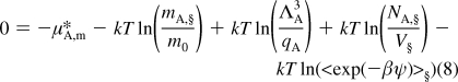Subtraction of eq 7 from eq 8 gives

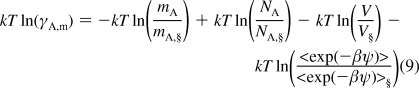The calculation of each term in eq 9 is straightforward, except for the last term, which is the difference of the solvation free energy of the inserted particle at a specified concentration from that of the most diluted solution.

As mentioned, previous attempts to calculate mean activity coefficients of alkali−halide salts were limited to implicit solvent methods using the potential mean force between molecules. Lyubartsev and Laaksonen derived the potential mean force using Smith and Dang’s NaCl(27) in flexible SPC water,(28) while Gavryushov and Linse used SPC/E water and Aqvist(29) and Dang’s parameters. Lenart(14) used Koneshan and Rasaiah parameters(30) for van der Waals interactions of ions, and the potentials in water were adjusted for a specifically designed implicit solvent model. Some of these approaches agree well with experiment. Experimental methods to measure mean activity coefficients are various, but the results are all very similar.(31) We used the values summarized the CRC Handbook(32) for comparison.

Diffusion coefficients of ions are usually calculated experimentally from their conductivities. In simulations, two methods to calculate them have been reported.¹⁵⁻¹⁹ The more intuitive method is direct calculation of the average mean square displacement of ions for a unit time period. Calculation of the velocity autocorrelation function also provides a link to the diffusion coefficient.(15) However, given long simulations, the two methods give equivalent results for the diffusion coefficients. In this research, we used the former method to calculate diffusion coefficients.

Information regarding the dynamics of ions in water is very limited and relies mostly on simulation. For example, the correlation time (or the residence time) of ion−water and ion−ion pairs can easily be calculated by simulation. Previous estimates of the residence times applied the autocorrelation function designed by Impey et al.(15) More recently, Laage and Hynes raised the issue that residence times calculated by that method are very sensitive to the tolerance time.(33) The tolerance time was originally introduced to the calculation in order to represent the transition state between the paired (reactant) and unpaired (product) states as the reactant state moves to become the product state. In other words, this catches the case when a pair only briefly becomes unpaired before pairing again, with a time period less than the tolerance time. The updated method by Laage and Hynes’ suggests calculating the new time correlation function (R(t)) based on the stable states picture model.(34) To apply this method, the states of stable reactant, R, (or paired) and stable product, P, (or unpaired) need to be defined. In the R state, molecule pairs are separated by almost the radius of the first shell (r_max1), which is the first peak of their radial distribution function (RDF, g). The two molecules in the pair reaches the P state when they are separated by almost the radius of the second shell (r_max2), which is the second peak of the RDF. The probability, p(t), is the probability that a molecule pair in R state at time 0 transforms into the P state after time t:

The residence time (τ) of the molecule pair is defined by the equation above. The bracket denotes average over the whole system and the whole period. It is assumed to be a single-exponent decay.

Although experimental measurements of the solubility of alkali−halide crystals in water are easily found, it is not simple to calculate solubility in simulation. To compare with experiment, it is necessary to estimate the equilibrium state of crystals in saturated solution. One means is by estimating the chemical potentials of both saturated solution and crystal. To do this, the chemical potential of the crystal and solutions at various concentrations is calculated and the concentration at which the two potentials are equal indicates saturation concentration.^24,35,36 Instead of this more tedious approach, we used a more direct method to derive the equilibrium state. Sufficiently large crystals in contact with an almost saturated ion solution will reach an equilibrium state given sufficient sampling. To avoid finite size surface effects of a small crystal, the crystal was assumed to be a two-dimensional periodic slab. We note that this approach, although direct, will likely require longer simulations to fully equilibrate the heterogeneous mixture. However, the direct method is advantageous since there are no underlying assumptions (as are required in the calculation of chemical potentials). As a result, it is expected that more accurate results can be obtained.

Methods

Molecular dynamics simulations were performed with the sander module of AMBER9^37,38 using the AMBER nonpolarizable potential energy function shown in eq 1. General conditions applied in all of the molecular dynamics simulations, unless otherwise stated, are discussed below. Direct space nonbond interactions were explicitly evaluated when the distance is below 9 Å. A 2 Å buffer was built into the pairlist, and rebuilding of the list was triggered if any particle moved more than 1.0 Å. Long-ranged electrostatic interactions were estimated with the particle mesh Ewald method,^39,40 and a homogeneous density approximation was applied to correct for the cutoff of the Lennard-Jones interactions. Particle grids for the Ewald summation were approximately one grid point per angstrom in each dimension. The atomic charges for the grid points were smoothed onto the grid using a fourth-order B-spline. Temperature and pressure were regulated by using weak coupling algorithm.(41) The coupling time for temperature and pressure control was 1 ps. The target temperature and pressure were 298 K and 1 bar, respectively. All of the water models used here are rigid, and the SHAKE algorithm(42) was applied to constrain all bonds to hydrogen with a tolerance of 10⁻⁵ Å. The time step for dynamics simulations was 2 fs. More detailed methods applied to the specific calculations are described below.

Activity Coefficients

The initial coordinates of water and ions were randomly positioned in a rectangular periodic box, which was prepared to have density of ∼1 g/cm³. The initial box size was about 38−40 Å, and the number of waters and ions in each case is displayed in Table 1. The systems were minimized by steepest descent for 1000 steps, followed by a two-step equilibration. In the first step, MD simulation was performed for 40 ps in the NVT ensemble. In the second step, 40 ps MD simulation was performed under NPT conditions. A cation−anion pair was inserted in the system slowly to calculate the hydration free energy of the ion pair. The insertion was carried out using thermodynamic integration. To facilitate the calculations, the insertion process was separated into three perturbation steps. In the first step, Lennard-Jones interactions of the inserted ion pair were turned on. In the second step, the charge of the cation was activated. In the last step, the charge of the anion was activated. The perturbation steps adopted the following mixing rule of the potential energy: U(λ) = f(λ)U₀ + (1 − f(λ))U₁, where U₀ and U₁ are the potential energy of the initial state and the final state. Intermediate states between perturbations were determined adjusting the parameter, λ (0 ≤ λ ≤ 1). For the first perturbation, f(λ) = (1 − λ)⁷∑⁶_{i = 0}λⁱ(6 + i)!/6!/i!, and for the second and third perturbations, f(λ) = 1 − λ was applied, respectively.^38,43 Numerous intermediate states between perturbations were defined by substituting λ with these numbers: 0.01, 0.05, 0.1, 0.15, 0.2, 0.25, 0.3, 0.35, 0.4, 0.45, 0.5, 0.55, 0.6, 0.65, 0.7, 0.75, 0.8, 0.85, 0.9, and 0.95 for the first perturbation and 0, 0.05, 0.1, 0.15, 0.2, 0.25, 0.3, 0.35, 0.4, 0.45, 0.5, 0.55, 0.6, 0.65, 0.7, 0.75, 0.8, 0.85, 0.9, 0.95, and 1 for the second and the third perturbations. Using the previously equilibrated coordinates, all of the states were simulated in the NTP ensemble to calculate <dU/dλ>. The initial 100 ps for each of the simulations was discarded. The <dU/dλ> values were fit into a cubic spline as a function of λ, and this was used to calculate ∫¹₀⟨dU/dλ⟩dλ numerically, which is equivalent to eq 6.

Table 1. Set of Simulations Performed for Calculating the Activity Coefficients^a.

KCl			NaCl
m	Nw	Nion	m	Nw	Nion
0.037	1500	1	0.037	1500	1
0.111	1497	3	0.111	1498	3
0.186	1493	5	0.186	1495	5
0.298	1489	8	0.298	1492	8
0.487	1481	13	0.486	1485	13
0.716	1473	19	0.713	1479	19
0.989	1460	26	0.982	1470	26
1.502	1441	39	1.489	1454	39
1.991	1422	51	2.006	1439	52
2.493	1403	63	2.495	1424	64
3.006	1385	75	2.992	1410	76
3.988	1350	97	4.017	1382	100
			4.998	1355	122

^aShown are the molalities (m) of KCl and NaCl solutions simulated when calculating the activity coefficients, including the number of explicit ion pairs (N_ion) and water molecules (N_w) in the periodic unit cell.

Diffusion Coefficients, Characteristic Radii of Water Shells, Cluster Population, and Residence Time

The initial coordinates of the water and ions were randomly placed in a rectangular periodic box keeping the density of the system to be ∼1 g/cm³. Fifteen hundred explicit water molecules and 27 ion pairs were added to make the concentration ∼1 m. The box sizes were approximately 36−40 Å. Note that LiF was omitted since its solubility is lower than 1 m.(32) Each system was minimized and equilibrated in the same way as described in the previous section, and then MD simulations were performed for 10 ns. Radial distribution functions (RDFs) were collected with the ptraj program in AMBER9. Each curve was smoothed using a Bézier curve to better obtain the characteristic radii of the RDF curves at dg/dr = 0. The three shortest radii were determined, and they were assigned sequentially as the radius of the first shell (r_max1; radius of the first peak), the radius of first coordination shell (r_min1; radius of the first minimum after r_max1), and the radius of the second shell (r_max2; radius of the second peak). The first shell was refined by repeatedly fitting the curve into quadratic equations.(11) The radius at the vertex of the quadratic fit was substituted for r_max1.

The relationship, 6D = lim_t→∞d<r²>/dt was utilized to calculate the diffusion coefficient (D).(44) Average mean-square displacement (<r²>) of each type of molecule up to 10 ps was plotted versus time every 1 ps. The curves were fit to a straight line that passes through the origin by least-squares. The slope of the line was regarded as 6D. The diffusion coefficients were then corrected for finite periodic box size effects as per Yeh and Hummer.(45) This was done by measuring the diffusion coefficients of ions with various sizes of the system, specifically 1500 water molecules and 27 ion pairs, 1000 water molecules and 18 ion pairs, and 500 water molecules and 9 ion pairs. These simulations were extended to 10 ns each. For the analysis of ion clusters, any ions located within r_min1 were considered to be linked. Groups of linked ions form ion clusters. Cluster populations were analyzed from the simulation of 1500 water molecules and 27 ion pairs.

Calculation of the residence time for a paired molecule requires the precise determination of the R and P states, which are based on the distance of the two molecules. The upper boundary of the R state (r_R) was the radius satisfying g(r_R) = √(g(r_max1)g(r_min1)). A pair of molecules at the same or shorter distance than r_R was considered to be in the R state. In a similar way, the lower boundary of the P state (r_P) was determined by the radius satisfying g(r_P) = √(g(r_min1)g(r_max2)). A pair of molecules separated by a distance equal or larger than r_P were defined to be in the P state. Originally, the lower boundary of the P state suggested by Laage and Hynes was the radius corresponding to the half-energy barrier in mean force potential curve. However, our definition of the boundary is equivalent to their definition because radial distribution is exponentially proportional to the potential of mean force (i.e., g(r) ≡ e^−w(r)/kT, where w(r) is the potential of mean force). The residence time, τ, was calculated by integrating the time correlation function Eq 10.

Because R(t) cannot be evaluated infinitely, the equation was integrated only from 0 to 1 ns and the rest of the integration was carried out under the assumption of exponential decay:

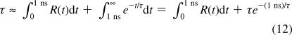Integration of R(t) over t was performed using the trapezoidal rule, and eq 12 was numerically solved to obtain τ.

Solubility

Rectangular crystals of alkali−halide salts were built using their lattice constants as described previously.(11) When building the NaCl-type crystals, the unit crystal was aligned exactly parallel to the rectangular axes (Figure 1A). On either side of the YZ planes of the crystals, an ion and water mixture with the density of ∼1.5−2.0 g/cm³ was prepared. The number of explicit ion pairs in the initial crystal was 500. Presaturated ion solutions were composed of roughly 20% more ion pairs than expected to be soluble in terms of molal concentration; 862 (LiCl), 266 (NaCl), 206 (KCl), 336 (RbCl), 901 (LiBr), 397 (NaBr), 246 (KBr), 304 (RbBr), 534 (LiI), 531 (NaI), 386 (KI), 336 (RbI), 1626 (CsF) ion pairs and 2000 water molecules. For the CsCl-type crystals (CsCl, CsBr, and CsI), the unit crystal was initially aligned to the rectangular axes then rotated 45° along the Z axis in order to reduce the net dipole along the X axis (Figure 1B). This prevented the strong net dipole from artificially breaking the crystal immediately after the start of the simulation. The number of explicit ion pairs in the crystal was 504. On either one of the YZ planes of the crystals, an ion and water mixture with the density of ∼1.5−2.0 g/cm³ was apposed; 120% saturated solutions and various other solutions at different concentrations were tried. However, we encountered several problems with CsCl-type crystals as explained in the next section.

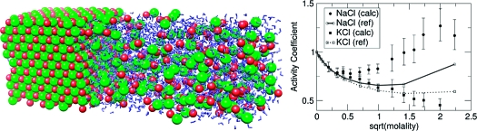
Figure 1.

Coexisting salt crystal and ion solution in a periodic box. The horizontal axis is the X axis, and ion solution was placed on one of the YZ planes of the crystals. (A) NaCl-type crystal and (B) CsCl-type crystal.

The equilibration and subsequent dynamics were normally not very sensitive to the precise setup of the crystal solution and its initial density. However, in a few cases, the crystal instantaneously disintegrated and melted into the aqueous solution due to instability in the built crystal; in these cases, the results were discarded. As the simulation cell is periodic, the initial setup constituted infinite crystal sheets with aqueous ion solution between the crystal sheets. The system was minimized by using the steepest descent method for 1000 steps and equilibrated at a constant temperature and pressure for 40 ps while harmonically restraining the coordinates of crystal ions to their initial positions with a force constant of 50 kcal/mol/Ų. Pressure was controlled by adjusting the periodic box size anisotropically so as not to break the connectivity of the crystals between neighboring boxes. That is, pressure applied to x, y, and z directions were calculated separately, and the three edges of the box were rescaled according to the three normal pressures. Anisotropic rescaling intrinsically requires longer equilibration time, but it is indispensible in nonisotropic systems like this. The coupling time for the pressure regulation was 1 ps. After removing the restraints, MD simulation was continuously performed and the crystals gradually grew or dissolved as they moved toward the equilibrium state.

The distribution of the water and ions along the X axis changes as the crystal grows or is dissolved. To obtain the distribution of molecules at different times in a consistent manner, a static reference needed to be defined. On the time scale of the MD simulations performed, the inner crystal layers remained intact. Therefore, we used the geometric center of the inner crystal layers as the reference point for the X axis distribution. From the reference point, the histogram of the molecules along the X axis was collected up to half of the X axis edge of the periodic box (x_max) with a step of 0.1 Å. Histograms along both the positive and negative directions of the X axis were averaged. This final histogram was converted to number density per unit volume by dividing by the volume of each bin of the histogram. The bulk molar concentration of the molecules in the solution was assumed to be the average molar concentration of the molecules located between x_max − 10 Å and x_max from the reference point. The volume and total potential energy of the system were traced and averaged. The system was considered to reach the equilibrium state when both the volume and potential energy leveled off. To avoid introducing biases when determining the equilibrium state, running averages over 60 ns of the two properties were recorded every 100 ps along with their standard deviation. The ranges that these averages cover with the tolerance of their standard deviations were compared each other. When the average overlap of the ranges from the last 40 ns onto the very last range is above 95%, we considered the system to be in equilibrium state (see Figure S1 in the Supporting Information). The final concentration of the solution phase was considered to be the average concentration of the last 30 ns.

Results and Discussion

Activity Coefficients

Activity coefficients of NaCl and KCl solutions at varying concentrations (≲5 m) were calculated with TIP3P water(8) and the TIP3P-compatible ions. Only this limited set was investigated as these simulations were very costly and effectively required the equivalent computer time of ∼11 700 days × 4 processors based on the performance of available clusters. Yet, these results still provide general insight into how much the activity coefficients from simulations vary with respect to experiment. To calculate activity coefficients, the number of explicit atoms in the periodic box was adjusted to simulate a variety of concentrations, as is shown in Table 1. In eq 9, all of the other parameters were determined (see Table 1) except for the excess chemical potential. The excess terms were estimated by TI of pair insertion. As the activities are very sensitive to small changes in the excess chemical potential terms, it is necessary to discuss how the error was estimated. In general, the errors of <dU/dλ>_i from the ith TI window can be estimated if the correlation length (τ_c) of <dU/dλ>_i is known.(46) Given this, we denoted the error as e_w,i, and it was estimated using the relationship

where (rmsd)_i is the rms deviation of <dU/dλ>_i and t_i is the length of the simulation required to obtain the rmsd. Although we did not precisely estimate the correlation length (τ_c) of <dU/dλ>_i for all of the TI windows, we expect that the correlation lengths are shorter than 1 ps (for example, please refer to the decay of the autocorrelation curve shown in Figure S2 in the Supporting Information). When we assume that the correlation lengths are less than 1 ps, the error estimates should be valid. As the simulations proceeded, it was noted that some windows had inherently low errors, dropping below 0.00001 kcal/mol within a few hundreds of picoseconds of simulation, whereas other windows required tens of nanoseconds before the error drops below 0.1 kcal/mol. The contribution of each window to the free energy change of a perturbation is roughly inversely proportional to the total number of windows (n_w) of the perturbation because the TI windows are almost evenly distributed. Therefore, an error in free energy calculation of each perturbation (e_p,j) is

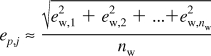where the subindex j denotes jth perturbation. The perturbations were composed of three steps. Finally, the error of the total free energy calculation (e_total) can be estimated as

We differentiated the time of simulations for the higher concentrations (>1 m) and the lower concentrations (<1 m) because we wanted higher precision at the lower concentrations. The finally estimated total errors fell around ±∼0.082 kcal/mol for the higher concentrations and ±∼0.034 kcal/mol for the lower concentrations. However, real errors might be even smaller because we assumed that τ_c was 1 ps, which is likely an overestimate.

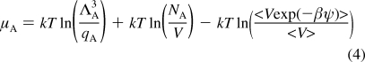
We now discuss the excess chemical potentials. The calculated excess chemical potentials are listed in Table S1 and displayed in Figure 2. In order to calculate activity coefficients of ion pairs applying eq 9, the difference in chemical potential from the most diluted solution is required. Due to the practical difficulty in carrying out simulations of high volume systems, with explicit solvent, we did not simulate solutions at less than 0.037 m. In fact, this is not sufficiently dilute, and we could not assume that the activity coefficient of the solution is unity at this concentration. When they are compared to experimental activity coefficients,(32) the chemical potential at this concentration is almost 0.1 kcal/mol more negative than that from the most diluted solution (i.e., − 0.1 kcal/mol ≈ kTln γ_m). This was approximately true for both NaCl and KCl. For this reason, we assumed that there is 0.1 kcal/mol difference in chemical potential at 0.037 m from the most diluted solution. In actuality, the values of the activity coefficients at the other concentrations are greatly affected by this number. However, choosing this number is reasonable, and regardless of the precise value, the overall shape of the curve of activity coefficients at various concentrations is preserved. The activity coefficients calculated with this assumption are listed in Tables 2 and S1.

Figure 2.

Calculated (calc) and experimental(32) (ref) mean activity coefficients of NaCl and KCl versus square root of molality. The X axis denotes the square root of molality of an ion pair, and the Y axis indicates its mean activity coefficients. Closed circles and closed squares denote the activity coefficients of TIP3P-compatible ion pairs, NaCl and KCl, in TIP3P water. Open circle and open squares are the experimental mean activity coefficients of NaCl and KCl in water.

Table 2. Activity Coefficients (γ) at Different Molalities (m) for NaCl and KCl Salt Solutions with the TIP3P-Compatible Ion Pairs.

NaCl	m	0.037	0.111	0.186	0.298	0.486	0.713	0.982	1.489	2.006	2.495	2.992	4.017	4.998
	γ	0.85	0.79	0.80	0.78	0.79	0.82	0.83	0.93	0.99	1.02	1.18	1.27	1.17
KCl	m	0.037	0.111	0.186	0.298	0.487	0.716	0.989	1.502	1.991	2.293
	γ	0.85	0.78	0.78	0.74	0.72	0.68	0.63	0.62	0.56	0.52

The insertion of ion pairs was composed of three perturbations. The contributions to the chemical potential from the three perturbations are indicated as μ_vdw, μ_elec1, and μ_elec2 (Table S1 in the Supporting Information). The μ_vdw generally increased as the concentration of the solution increased for both NaCl and KCl. For μ_elec1, the insertion of sodium ions was less favored as concentration increased; however, it became more favored for potassium ions beyond 1 m. Overall, the contributions to the differences in the chemical potentials observed were relatively small (columns 2, 3, and 4 in Table S1 in the Supporting Information) with the exception of the hydration free energies. The calculated activity coefficients deviate from the experimental values as the concentration increases (Table 2). However, the curve of NaCl was placed above that of KCl, which qualitatively corresponds to the experimental curves. Although we will discuss solubility further below, the solubility of NaCl and KCl determined by simulations in TIP3P water was actually lower than their experimental solubility. However, we did not observe crystal formation on the time scale of these simulations, suggesting the solutions were supersaturated above certain concentrations.

Previous investigations determined the activity coefficients of NaCl and KCl using effective interaction potentials.^12,13 Lyubartsev and Laaksonen calculated the activity coefficients of Smith and Dang’s NaCl(27) in flexible SPC water.(28) The results are very impressive as their numbers are very close to the experimental mean activity coefficients, even up to 5 M. Both observations imply that potential energies among Smith and Dang’s Na⁺, Cl⁻, and SPC/E water are reasonably balanced and can properly estimate the activity coefficient and the solubility. However, this does not sufficiently support the idea that all of the Smith−Dang−Garrett ions^27,47−50 are appropriately balanced. We note that it is also possible that the flexible SPC water model provides better effective interaction potentials than SPC/E. Gavryushov and Linse applied a similar methodology to Lyubartsev and Laaksonen, except that they used spherical boundary conditions and the SPC/E fixed-point water model. They determined mean activity coefficients of Aqvist’s ions(29) (Na⁺ and K⁺) in addition to Smith and Dang’s ions. Note that the activity coefficients of NaCl generally correspond to the true activity, regardless the source of the ion parameters, while those of KCl tend to poorly reproduce the experimental activity coefficients. This likely results from inaccurate estimates of the solubility of KCl in simulation with available parameters compared to experiment. Lenart et al.(14) simulated ion solutions with a specially designed implicit solvent model that included a distance-dependent dielectric permittivity, and this led to improved results. However, it should be noted that they did not use a standard combining rule for the Lennard-Jones potential and instead defined separate Lennard-Jones interactions between all of the atom pair types. This suggests that current pair potentials still have room for improvement in the context of doing away with the simple combining rules.

Diffusion Coefficients and Population of Ion Clusters

Experimental and computed diffusion coefficients of alkali and halide ions at infinite dilution are listed in Table 3 and compared with those from pre-existing ion models. The diffusion coefficient increases as the size of ion increases with characteristic peaks at Rb⁺ and Br⁻. Although previous work claims to reproduce the qualitative trend of the diffusion coefficients with the Smith−Dang−Garrett ion parameters, we were not able to reproduce those results.^16,17,19 We only found the characteristic peaks with the water-model-specific cation parameters in SPC/E. The differences likely relate to differences in how the long-range electrostatic interactions were determined and the correction for the finite size effects. Moreover, in the current work, larger periodic unit cells were applied, which may also partially explain the difference. Until our recent work, pair potentials for the ions were largely independent of applied water model. Yet, it is well-known that TIP3P water diffuses too rapidly and this in turn leads to ions that are too swift in TIP3P water. Consequently, experimental diffusion coefficients are better reproduced in TIP4P_EW and SPC/E water, although there still are significant discrepancies. These discrepancies partially result from concentration effects as the simulations were performed in 1 m solution while the experimental numbers are from dilute solution. When the concentration of the ions in solution increases, the diffusion coefficients of the ions decrease.(18) Diffusion coefficients of the ions also appear to depend on the choice of counterion as ions tend to move swifter when they are solvated with fast-moving counterions (see Table S2 in Supporting Information). Generally, if the counterion is larger, the increment in the diffusion coefficient is greater. Considering the relative diffusion rates of the ions and water molecules, swift molecules tend to pull or push the ions and thus enhance the diffusion coefficients of the ions. However, this is not always true. TIP3P-compatible Rb⁺ is fastest with Br⁻ rather than the larger I⁻ ion. Also, SPC/E-compatible Br⁻ diffuses most rapidly with K⁺ and Rb⁺. Looking at the residence time between cation and anion (shown in the next section), the results suggest that high residence times impede the movements of both the cations and anions (because the paired ions are effectively heavier). Generally, the larger ions have higher diffusion coefficients; however, the relative values are influenced by ion pairing and the diffusion rates of other molecules in the solution.

Table 3. Experimental and Computed Diffusion Coefficients (D × 10⁻⁵ cm²/s) of Alkali and Halide Ions in Aqueous Solutions at 25 °C^a.

	water-model-specific ions(11)			Smith−Dang−Garrett ions (Li+,(47) Na+,(27) K+,(48) Rb+,(48) Cs+,(49) F−,(47) Cl−,(48) I−50)
	TIP3P	TIP4PEW	SPC/E	TIP3P	TIP4PEW	SPC/E	exp
Li+	2.31	1.30	1.30	2.53	1.39	1.38	1.029
Na+	2.28	1.12	1.34	2.22	1.20	1.31	1.334
K+	3.14	1.72	1.89	3.30	1.92	2.05	1.957
Rb+	3.36	1.93	2.05	3.31	1.97	2.06	2.072
Cs+	3.40	2.05	1.99	3.44	2.08	2.12	2.056
F−	2.02	1.05	1.09	1.27	1.04	1.07	1.475
Cl−	2.90	1.52	1.66	3.08	1.64	1.76	2.032
Br−	3.22	1.67	1.78				2.080
I−	3.42	1.76	1.81	3.42	1.75	1.94	2.045

^aDiffusion coefficients were calculated at 1 m concentration with the counter ions Cl⁻ and Na⁺. Note that the experimental diffusion coefficients(32) represent dilute solution. Diffusion coefficients computed with other counter ions are displayed in the Supporting Information. The diffusion coefficients before correcting for finite size effects are also provided in the Supporting Information.

Even when ions are completely dissolved in water, ions constantly form transient clusters. The population of these clusters (displayed in Table S4 in the Supporting Information) is closely related to the other dynamic properties of the solution.(51) From the data, the association constant for each single cation−anion pair was calculated. The true association constant is the ratio of the activity of ion pair to the activities of each of the single ions (K = a_pair/(a_cation × a_anion)). Due to the overwhelming computational demands of estimating activities for each of the ion models, we assumed the activities were unity and substituted mole fraction, molar concentration, and molal concentration. This implies that the calculated association constants are not accurate. Table 4 shows the simplified association constants in terms of molal concentration. The association constants in terms of molar concentration are similar and are reported in the Supporting Information. Chen and Pappu(52) performed a similar analysis using Åqvist ions(29) where the association constants were calculated in terms of molal concentration. When these numbers are compared with Fuoss’ conductimetry results,(53) the results suggest that the combination of Åqvist cations with the anions from Chandresekhar et al.(54) and Lybrand et al.(55) is excellent. However, this analysis neglected the activity coefficients. As shown in Chen and Pappu’s Table 3, the association constant is clearly greater when concentration is low, which proves activity coefficients cannot be ignored. The association at the low concentration is indeed close to the actual association constant because activity coefficients are close to unity at low concentrations. If ion-dipole effects are neglected, the activity coefficients of ion pairs are almost unity. If we take experimental mean activity coefficients for single ions from NaCl and KCl, they are 0.779 and 0.768 at 0.1 m. Therefore, 1.65 (=1/0.779²) for NaCl and 1.70 (=1/0.768²) for KCl should be multiplied to their calculations. In other words, their calculations were underestimated by 65−70%. Table 5 shows Fuoss’s association constants. Association constants of water-model-specific ions, and Smith−Dang−Garrett ions are shown in Table 4, and generally the values were far less than Fuoss’ association constants even though these numbers are probably underestimated. Fuoss estimated the numbers based on the conductometric data assuming that the paired ions play no effective role in conductance of the ionic solution. Essentially, the conductance of alkali−halide solutions was extrapolated to infinite dilution. However, consistent with Chen and Pappu, we assume that the distances between ion pairs are within r_min1. In other words, only contact ion pairs were considered as ion pairs. However, Gurney radii from Fuoss’ data (see Fuoss’ Table 2), which are arguably the criterion determining free ion and ion pair, are generally much greater than our r_min1 values, especially for Li-, Na-, and K-associated salts, although the distances for some Rb- and Cs-associated salts are slightly shorter than our r_min1 values. For this reason, his nonconductive ion pairs possibly include some solvent-shared pairs as well as contact ion pairs. The association constants were recalculated using the criteria provided by Fuoss to see how much the association constants change depending on the criteria (Table S5 in the Supporting Information). Although significant differences from Fuoss’ estimation were still observed, the new association constants agreed much better with Fuoss’ numbers. With the same assumptions, most of the association constants of Åqvist’s ions calculated by Chen and Pappu would exceed Fuoss’ estimation. It is not clear why the Åqvist ions, compared to the other ion models, show such significant differences.

Table 4. Association Constants of Cation−Anion Pairs at 1 m^a.

salt	TIP3P		TIP4PEW		SPC/E
	water-model-specific ions
LiCl	0.48	±0.17	0.026	±0.044	0.0037	±0.011
LiBr	0.085	±0.059	0.015	±0.029	0.0020	±0.0085
LiI	0.0077	±0.017	0.0035	±0.012	0.00053	±0.0044
NaF	0.14	±0.082	0.012	±0.022	0.022	±0.028
NaCl	0.12	±0.072	0.029	±0.031	0.020	±0.028
NaBr	0.090	±0.062	0.031	±0.035	0.024	±0.030
NaI	0.048	±0.043	0.027	±0.033	0.021	±0.029
KF	0.19	±0.097	0.074	±0.057	0.096	±0.063
KCl	0.28	±0.12	0.17	±0.092	0.14	±0.081
KBr	0.30	±0.13	0.22	±0.10	0.16	±0.087
KI	0.26	±0.12	0.23	±0.11	0.17	±0.090
RbF	0.18	±0.092	0.081	±0.057	0.13	±0.078
RbCl	0.32	±0.14	0.23	±0.11	0.23	±0.11
RbBr	0.34	±0.14	0.29	±0.13	0.26	±0.12
RbI	0.33	±0.14	0.35	±0.15	0.29	±0.13
CsF	0.19	±0.095	0.13	±0.078	0.29	±0.13
CsCl	0.39	±0.16	0.37	±0.15	0.87	±0.32
CsBr	0.44	±0.18	0.53	±0.20	1.0	±0.39
CsI	0.47	±0.18	0.59	±0.22	1.1	±0.47
	Smith−Dang−Garrett ions
LiCl	0.059	±0.053	0.081	±0.061	0.023	±0.030
LiI	0.0012	±0.0066	0.0024	±0.0099	0.0012	±0.0066
NaF	0.48	±0.49	0.19	±0.10	0.23	±0.11
NaCl	0.10	±0.066	0.12	±0.069	0.084	±0.059
NaI	0.035	±0.038	0.063	±0.054	0.041	±0.040
KF	0.23	±0.11	0.12	±0.073	0.18	±0.093
KCl	0.49	±0.20	0.58	±0.22	0.53	±0.20
KI	0.49	±0.19	0.85	±0.33	0.70	±0.27
RbF	0.20	±0.10	0.12	±0.074	0.18	±0.092
RbCl	0.60	±0.23	0.70	±0.26	0.68	±0.26
RbI	0.67	±0.26	1.1	±0.46	0.96	±0.36
CsF	0.17	±0.088	0.11	±0.071	0.17	±0.090
CsCl	0.77	±0.28	0.94	±0.34	0.94	±0.34
CsI	1.0	±0.41	1.9	±0.80	1.5	±0.61

^aIon concentrations listed in Table S4 of Supporting Information were used to calculate the constants in terms of both molal concentration. The unit of the constants is m⁻¹. The deviations were calculated from the deviations of the individual populations in Table S4 of Supporting Information. Some of these are very large. However, they are intrinsic since the cluster populations fluctuate considerably.

Table 5. Fuoss’s Estimation of the Association Constants of Alkali−Halide Salts in Water(53).

	Li	Na	K	Rb	Cs
F	1.97	0.85		0.30	0.49
Cl	0.75	0.82	0.53	0.24	0.62
Br	0.71	0.73	0.44	0.23	0.54
I	0.54	0.60	0.40	0.24	0.50

Ion−Water Structure and Residence Time

The residence time between two molecules is an indicator of the lifetime of pair association at a particular temperature. We calculated residence times of cation−anion, water−cation, and water−anion pairs in 1 m solutions using water-model-specific and Smith−Dang−Garrett ion models. The results are listed in Table S6 in the Supporting Information. The characteristic radii from the RDF were used in the determination of the residence time and are listed in the Supporting Information (Table S3). The residence times between Li⁺ and F⁻ are considered to be very long (compared to the MD simulation time scale), and thus we could not estimate their values. Also, we could not calculate the residence time between TIP4P_EW-compatible Cs⁺ and F⁻ and Smith−Dang−Garrett Cs⁺ and F⁻ in SPC/E water because of an insufficient size for the ensemble. Consistent trends in the cation−anion residence times across a particular column or row of the table (as a function of the ion sizes) are not observed. When the cation is fixed (along the column in Table S6A in the Supporting Information), the curves of the residence times generally monotonically increase, monotonically decrease, or display a convex shape with a single maximum. For the TIP3P-compatible cations Li⁺ and Na⁺, the residence times monotonically drop as the size of the paired anions increases. K⁺ and Rb⁺ have maximal residence time with Br⁻, whereas Cs⁺ does with I⁻. The trend is similar with the TIP4P_EW-compatible cations. However, here Na⁺ has a maximal residency time with Br⁻, while K⁺, Rb⁺, and Cs⁺ have their peaks with I⁻. SPC/E-compatible cations behave slightly differently from the ions of the other models. Na⁺ (and possibly Li⁺) ions have both local minimum and maximum with Cl⁻ and Br⁻, respectively. However, Smith−Dang−Garrett cations do not have such maxima in the middle of the series. When the cation is smaller than Na⁺, cation−anion residence times continuously decrease as the size of the anion increases. When the cation is larger than K⁺, residence times tend to increase as a function of the anion size. These behaviors consistently can be observed in the three different types of water models. On the other hand, in the series of anions (along the row in Table S6A in the Supporting Information), the curves of the residence time generally show two patterns: monotonous decrease or concave shape having one minimum. The minimums are located at slightly different positions depending on the anion and ion models. All the TIP3P-compatible anions have the longest residence time when they are paired with Li⁺. The residence times in the series gradually decreased as the size of the pairing cations increases excluding I⁻, which has a slight increase compared with Cs⁺. TIP4P_EW-Li⁺ also displayed the longest residence times with any pair of anions. However, in the series of Br⁻ and I⁻, the shortest residence times were reached at Rb⁺. Minimums of residence times also can be observed with all the SPC/E-compatible anions; F⁻ with K⁺, and the other anions with Na⁺. For the Smith−Dang−Garrett anions, such minimums were only observed with I⁻ when it is solvated in TIP3P or TIP4P_EW water. Unexpectedly, the residence time of I⁻ with these parameters in SPC/E shows an increasing pattern as a function of cation size. Overall, the residence times are complicated and depend on both the ion parameters and the applied water model. The largest variance was seen with the TIP3P water model.

Residence times between cations and water molecules (Table S6B in the Supporting Information) show little dependence on the size of the counterions. Unlike cation−anion residence times, the average water−cation residence times generally are not strongly sensitive to the choice of ion force field, although this appears to be less true with Li⁺ and Na⁺. However, the differences among anion−water residence times with different ion models are small, even with the smallest anion, F⁻ (Table S6C in the Supporting Information). These observations are confusing because, while significant influence of the water and ion parameter model is observed for anion−cation interactions, little is observed with ion−water residence times. This likely results from the heavy focus on ion−water interactions, as compared to ion−ion, in force field development. Although our work in the development of water-model-specific ion models did include ion−ion interactions, specifically, the crystal lattice energy and lattice constant, the ion−ion residence times lack consistency. On the other hand, residence times of ion−water pairs (τ_w−i) are closely related with the diffusion coefficients of ions (D_i) and water molecules (D_w). This can be seen when D_i and D_w/τ^1/2_w−i are plotted in an ad hoc manner to show relationships among the data; when this is done, a roughly linear correlation is observed (Figure S3 in the Supporting Information). Interestingly, the slopes of the linear relationship are almost identical no matter what ion or water models are used. However, the diffusion rates clearly depend on the concentration of the ions and also the nature of the cation−anion and water−water interactions.

Solubility

Unexpected crystallization of alkali−halide salts at concentrations below their saturation limit motivated our development of new ion parameters.(11) A necessary test of these parameters is alkali−halide pair solubility. Initially, we attempted to calculate the solubility of every pair of alkali−halide salts. However, we observed problems with salts paired with lithium or cesium ions. Transitions in the crystal structures, detected by sudden change of volume or potential energy, were observed. Also, the structures of the newly growing crystals on the surface of the pre-existing crystal were different from their natural crystal structure. Another problem was exposed in salts paired with fluoride ions. The volume and the potential energy of the systems fluctuated at low frequency. Although the systems may satisfy the condition of equilibrium as described in the Methods section, in this case, the equilibrium states were suspicious because of the low-frequency fluctuations of the two properties. For these reasons, we only show the valid solubility results in Table 6.

Table 6. Solubility of Alkali-Halide Salts Determined by Simulations Using Various Water and Ion Models.M and m Denote Molar Concentration and Molal Concentration, Respectively. The Sub-Indices, ‘w’ and ‘s’ Denote Water and Solute. Experimental Solubilities(32) are Reported in Terms of Molal Concentration at 298K.

salt	Mw		Ms		ms		ref
TIP3P/TIP3P-compatible ions
NaCl	53.67	±0.14	1.49	±0.02	1.54	±0.02	6.15
NaBr	48.15	±0.15	4.47	±0.03	5.15	±0.04	9.19
NaI	41.14	±0.21	5.67	±0.04	7.66	±0.07	12.28
KCl	53.61	±0.17	0.96	±0.01	0.99	±0.01	4.77
KBr	53.48	±0.13	0.79	±0.01	0.82	±0.01	5.7
KI	50.59	±0.12	1.54	±0.01	1.69	±0.02	8.92
RbCl	51.07	±0.14	2.37	±0.02	2.58	±0.02	7.76
RbBr	50.65	±0.11	2.01	±0.02	2.21	±0.02	7.04
RbI	49.76	±0.12	1.71	±0.02	1.91	±0.02	7.78
TIP4PEW/TIP4PEW-compatible ions
NaCl	48.68	±0.21	6.05	±0.06	6.90	±0.07	6.15
NaBr	45.03	±0.17	6.44	±0.05	7.94	±0.07	9.19
NaI	36.94	±0.17	7.62	±0.06	11.44	±0.10	12.28
KCl	49.63	±0.18	3.57	±0.03	3.99	±0.04	4.77
KBr	51.57	±0.19	1.89	±0.02	2.03	±0.03	5.7
KI	49.52	±0.15	2.04	±0.02	2.29	±0.03	8.92
RbCl	44.60	±0.13	5.46	±0.04	6.80	±0.05	7.76
RbBr	48.64	±0.15	2.91	±0.03	3.32	±0.04	7.04
RbI	50.64	±0.14	1.53	±0.01	1.68	±0.02	7.78
SPC/E/SPC/E-compatible ions
NaCl	48.04	±0.15	6.29	±0.06	7.27	±0.07	6.15
NaBr	44.16	±0.19	6.66	±0.05	8.37	±0.07	9.19
NaI	35.66	±0.17	7.81	±0.05	12.17	±0.10	12.28
KCl	48.15	±0.15	4.44	±0.04	5.11	±0.05	4.77
KBr	49.74	±0.12	2.77	±0.03	3.09	±0.03	5.7
KI	47.87	±0.13	2.60	±0.02	3.02	±0.02	8.92
RbCl	46.72	±0.20	4.56	±0.04	5.41	±0.05	7.76
RbBr	48.93	±0.13	2.82	±0.02	3.20	±0.03	7.04
RbI	49.69	±0.12	1.85	±0.02	2.07	±0.02	7.78
TIP3P/Smith−Dang−Garrett ions
NaCl	49.63	±0.17	4.32	±0.05	4.84	±0.05	6.15
NaI	30.62	±0.20	8.38	±0.06	15.19	±0.15	12.28
KCl	54.14	±0.12	0.48	±0.01	0.49	±0.01	4.77
KI	51.25	±0.13	1.09	±0.02	1.18	±0.02	8.92
RbCl	54.03	±0.13	0.49	±0.01	0.50	±0.01	7.76
RbI	53.06	±0.13	0.54	±0.01	0.57	±0.01	7.78
SPC/E/Smith−Dang−Garrett ions
NaCl	49.04	±0.21	4.91	±0.04	5.56	±0.05	6.15
NaI	32.37	±0.18	7.94	±0.06	13.61	±0.12	12.28
KCl	54.64	±0.18	0.52	±0.02	0.53	±0.02	4.77
KI	52.88	±2.98	0.98	±1.48	1.03	±1.56	8.92
RbCl	54.25	±0.18	0.65	±0.02	0.67	±0.02	7.76
RbI	55.23	±2.31	0.21	±0.05	0.21	±0.05	7.78

Depending on the choice of ion pair and ion parameters, simulations required about ∼110−530 ns for the solution crystal coexisting systems to reach their equilibrium states. This simulation time could, in principle, be reduced if the initial concentration and density of the solution opposed with the crystal are very close to its saturation condition. Notwithstanding, it is presumed that at least 100 ns of simulation are required. The equilibrium concentrations of the cation and the anion in the same system were almost identical as expected. Thus, the concentrations of the paired salt shown in Table 6 are the average of the cation and the anion. The molar concentration of water is also affected by the concentration of salts. Molality was calculated according to the molar concentration of both salt and water.

A solution becomes saturated when the chemical potentials of crystal and solution are equal. The chemical potentials of crystals can be assumed to be constants because the dependency of chemical potential of crystal on its size is usually negligible. However, the chemical potential of solution significantly increases as the concentration increases. The low solubility of the TIP3P-compatible ions implies that the chemical potential of the crystals are too low in general because at low concentration the deviation of the activity coefficients from the experimental results is small, as shown in Figure 2, and the deviation of chemical potential of the solution from the real solution might be small. Although the absolute solubility values of the TIP3P-compatible ions deviate significantly from experiment, the qualitative solubility trends are most accurately reproduced with these parameters compared to the other models (Table 6). Smith−Dang−Garrett ions also showed low solubility in TIP3P water, except for NaI, which had a higher solubility than true NaI solution. However, the qualitative trends were not observed with Smith−Dang−Garrett ions in TIP3P water: NaCl and NaI were relatively good, but the other salts showed significant deviation. TIP4P_EW-compatible ions well reproduced the saturation concentrations with Na-associated or Cl-associated salts. SPC/E-compatible ions showed similar behaviors with Na-associated or Cl-associated salts, but the solubilities were not as accurate as TIP4P_EW ions. Smith−Dang−Garrett ions did not behave much differently in SPC/E water than they did in TIP3P water. They showed relatively good solubilities with NaCl and NaI. Since the ion models are identical for the Smith−Dang−Garrett ions, the chemical potential of the crystals are presumably the same in both water models. In addition to this, as the solubility is not strongly affected by the water models, the chemical potential of the solution as a function of concentration is likely also almost identical regardless of the choice of water model. As a result, we can presume that the activity coefficients do not change greatly as a function of concentration in different water models as long as the ion models are identical. However, absolute hydration free energies can be different.(11) The various simulation sets except TIP3P/TIP3P-compatible ions have one characteristic in common. Their solubilities were generally well reproduced with NaCl. However, as the relative distance from NaCl becomes farther, the deviation of the solubilities seems to increase.

To better understand the deviations in solubility compared to experiment, we studied the effects of lattice energy on the solubility. Lattice energy is the potential energy difference generated when ions in a crystal are separated to infinite distance. A plot of the difference in experimental and calculated lattice energies versus the natural log of the ratio of calculated and experimental molal concentrations exposes trends for the different ion model parameter sets (Figure 3). If good agreement between the experimental and calculated values in both properties is obtained, the points will tend to cluster about the origin. The data suggest that the errors in the lattice energies for the various salts calculated using Smith−Dang−Garrett ions are generally positive (calculated < experiment) in contrast to water-model-specific ions.(11) Interestingly, regardless of the sign of the deviation in the lattice energy, most of the data points are located above X axis. This suggests that the solubility values calculated were generally lower than experiment. The data in the figure also suggest that greater absolute deviations between experiment and calculation of the lattice energy tend to lead to greater deviations in the solubility. However, there are trends in the deviations of the lattice energy that depend on the choice of cation. With the water-specific ion parameters, Na-associated salts were less sensitive to the deviation of lattice energy (solid line) while Rb-associated salts were much more sensitive (dashed line). K-associated salts were located in the middle (dotted line). Although there is a slight discrepancy regarding the extent of the effect, the solubility of Smith−Dang−Garrett salts was similarly affected by the deviations of lattice energy, and the effects were also distinctive depending on the cations. In conclusion, the solubility of salts is closely correlated to the deviation of lattice energy. We tried to find correlations of solubility with lattice constants, but we could not find obvious correlations. These results suggest that the parametrization of the TIP3P-compatible ions can be revisited to improve salt solubilities by focusing more heavily on reproducing the lattice energy.

Figure 3.

The effects of the deviations of the lattice energy on the solubility. X axis indicates the difference of the lattice energy calculated (LE_calc) from the experimental lattice energy (LE_ref).(11)Y axis indicates the logarithmic ratio of experimental saturation concentration (m_ref) to the calculated saturation concentration (m_calc) in terms of molality. Each point denotes the alkali−halide salts, as shown in the legend on the right-hand side. Different colors specify the ion and water models: blue for TIP3P-compatible ions in TIP3P water, magenta for TIP4P_EW-compatible ions/TIP4P_EW water, yellow for SPC/E-compatible ions in SPC/E water, cyan for Smith−Dang−Garrett ions in TIP3P water, and violet for Smith−Dang−Garrett ions in SPC/E water. Among them, water-model-specific ions were fit to y = ax² curves, where a is a fitting parameter. The solid line, the dotted line, and the dashed line are the fit curves for Na-associated salts, K-associated salts, and Rb-associated salts.

Figure 4 shows the correlations between the association constants of alkali−halide pairs (listed in Table 4) and their solubility. Generally, the two properties were inversely proportional, such that ion pairs with higher association constants have a greater tendency to form crystals. Fuoss’ association constants do not show this correlation (Figure 4B); however, as discussed, their Gurney radii might not be able to distinguish contact ion pairs from solvent-shared pairs, which means the reported association constants also include non-crystal-forming associations. In any case, the correlation between the calculated cluster populations and the saturation concentrations is useful since the more easily calculated association constant can be utilized to estimate solubility.

Figure 4.

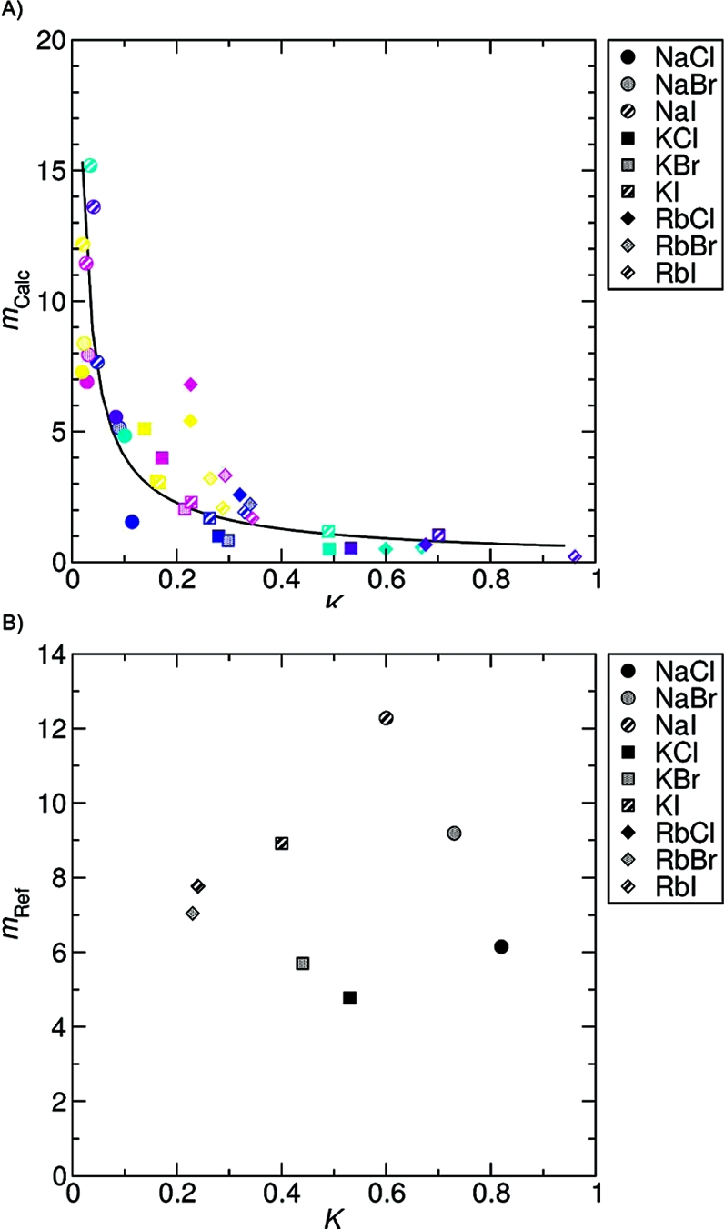
Correlation of the association constant (K) of cation−anion pair to the saturation concentration (m). Calculated molal saturation concentrations of salts are inversely proportional to the association constant of the ion pair (A). The solid line indicates the fitted curve, m_calc = 0.593K^−0.835 (R² = 0.7618). The color scheme is same as that in Figure 3. However, the experimental saturation concentrations(32) did not show correlation with Fuoss’ association constants(53) (B).

Figure 5 shows a clear correlation between the residence times and solubility. The results suggest that high cation−anion residence times drive the ions in solution toward the crystal form, whereas high water−cation and water−anion residence times tend to dissolve the crystal (see the legend of Figure 5). Although the results appear reasonable, these observations cannot be experimentally validated as we do not have an experimental measure of the residence times.

Figure 5.

Correlation of the residence times to the saturation concentration. Under the assumption that the inverse of residence time is proportional to the dissociation rates, and that the pairing between ion−water and ion−ion is a first-order reaction implying that the association constants are the ratio of the rates of the forward and backward reactions, the calculated molal saturation concentrations of alkali−halide salts (m_calc) were plotted against τ_c-a/τ_w-a × τ_w-c. Here τ_c-a, τ_w-c, and τ_w-a are residence times of cation−anion, water−cation, and water−anion, respectively. The solid line indicates the fitted curve of all the data points, y = 0.460x^−1.028 (R² = 0.7656). The color scheme is same as that in Figure 3.

By investigating these correlations, the links among the properties—including diffusion coefficients, residence times, association constants, and solubility—become clearer. Focusing on the ion−water interactions, Figure S3 in the Supporting Information shows that the diffusion coefficients of the ions are largely dependent on the choice of water model. Also, looking at the Smith−Dang−Garrett ions in Table S6B,C in the Supporting Information, the ion−water residence times also depend on the choice of water model. The dependency of the residence times on the choice of water model was generally in the order, water−anion < water−cation < cation−anion, as shown in Table S6 in the Supporting Information. When we assume that the water−anion and water−cation residence times can be correctly calculated, this suggests a critical need to balance the ion−ion interactions. This balance between the residence times is also closely related to the solubility, as shown in Figure 5, and even to the association constants based in Figure 4. Originally, water-model-specific ion models were optimized using multiple properties reflecting ion−ion interactions. In spite of the effort, cation−anion residence times, association constants, and solubility show large variability depending on the choice of water model. This, along with the sensitivity of the solubility to the lattice energy (Figure 3), again emphasizes the importance of ion−ion interactions in the parametrization of ion force fields.

The relevance of each of these properties (diffusion coefficients, residence times, lattice energy, association constants, and solubility) to the activity coefficients was not assessed in detail here as the limited set of calculations performed was extremely computationally demanding. However, on the basis of previous work, relationships can be estimated. The activity coefficients of the Smith−Dang−Garrett ions calculated by Gavryushov and Linse(12) suggest that the calculated NaCl activity coefficients are relatively good compared to KCl. Table 6 also suggests solubility is better reproduced with NaCl. These results suggest that, if solubility is accurately simulated, the activity coefficient should also be accurately reproduced. The TIP3P-compatible ions showed the highest deviations from true solubility. Therefore, the TIP3P-compatible ions should not be used for simulations at high salt concentrations. Although Smith−Dang−Garrett ions are fine with NaCl, their KCl is not appropriate for simulating high salt environments. For this reason, we recommend TIP4P_EW and SPC/E water models together with their water-model-specific ions for simulating high salts concentration.

Conclusion

The dynamic and energetic properties of alkali and halide ions were calculated in simulation using various different ion and water force fields including our previously developed water-model-specific ion parametrizations.(11) Mean activity coefficients were determined for NaCl and KCl in TIP3P water. This required extensive simulation at multiple salt concentrations. Qualitatively, the mean activity coefficients correspond to experiment; however, the deviations tend to increase as the salt concentration increases. Although extremely computationally demanding, to better determine which model is most appropriate for reproducing the experimental activity coefficients, all of the pairs of alkali−halide salts should be investigated using explicit solvent with the various parameter sets. However, these and previous results do clearly suggest that accurate estimation of solubility is critical to accurately calculate activity. Diffusion coefficients appear to be largely dependent on the choice of water model. Generally, faster moving water models resulted in higher diffusion coefficients for the solvated ions, but at the same time, the diffusion constants were almost inversely proportional to the square root of the residence time between the ion and the water molecule. We also calculated the association constants of various alkali−halide salts in terms of molar and molal concentration. Comparison with experimental association constants revealed that our numbers are seriously underestimated. However, the lower association constants could be explained by two reasons, specifically (1) since Fuoss’ experimental data use a greater cutoff length defining ion pairs which may include solvent-separated pairs, and (2) if activity coefficients are properly considered, our calculated association constants in terms of molar and molal concentration would increase. The residence times between ion and water and ion and ion were also calculated. Ion−ion residence times varied significantly according to the choice of water model, while the ion−water residence times did not. The solubilities of most of the alkali−halide salt pairs were estimated. The TIP3P-compatible ions showed qualitatively correct differences among the various salts, but the solubilities were generally significantly underestimated. The TIP4P_EW and SPC/E ion parameter models well reproduced the solubilities of Na-associated salts and Cl-associated salts. Smith−Dang−Garrett ions also qualitatively reproduced the solubilities of NaCl; however, the deviations of the other ions in the parameter sets from experimental were generally greater than observed with the TIP4P_EW- and SPC/E-compatible ion parameters.

Some of the dynamic and energetic properties of alkali and halide ions show a strong dependence on the choice of water model. Therefore, designing reliable water models is important. Ion force fields can then be developed on top of that foundation with care to balance the ion−ion interactions as many pairwise properties such as the association constant, the cation−anion residence time, and the solubility are very sensitive to these. In summary, the results suggest that our SPC/E and TIP4P_EW water-model-specific ion parameters fairly accurately model the behavior of the monovalent ions in aqueous solution across a wide range of concentrations, whereas the TIP3P-compatible ion parameters should be avoided at high salt concentrations.

Supporting Information Available

Additional information including (a) pictorial description of how precise overlaps were monitored, (b) autocorrelation curves of dU/dλ, (c) correlations of diffusion coefficients and residence times, (d) complete tables of the chemical potentials and terms evaluated to estimate activities, (e) diffusion coefficients for 1 m solutions with each ion pair combination, (f) characteristic radii of the ion−ion and ion−water interactions, (g) ion pair cluster configurations, (h) association constants for cation−ion pairs, and (i) ion pair residence times. This material is available free of charge via the Internet at http://pubs.acs.org.

Funding Statement

National Institutes of Health, United States

References

- Manning G. S. Q. Rev. Biophys. 1978, 2, 159. [DOI] [PubMed] [Google Scholar]
- Sinibaldi F.; Howes B. D.; Smulevich G.; Ciaccio C.; Coletta M.; Santucci R. J. Biol. Inorg. Chem. 2003, 8, 663. [DOI] [PubMed] [Google Scholar]
- Auffinger P.; Bielecki L.; Westhof E. Structure 2004, 12, 379. [DOI] [PubMed] [Google Scholar]
- Klein D. J.; Moore P. B.; Steitz T. A. RNA 2004, 10, 1366. [DOI] [PMC free article] [PubMed] [Google Scholar]
- Sissi C.; Chemello A.; Noble C. G.; Maxwell A.; Palumbo M. J. Mol. Biol. 2005, 353, 1152. [DOI] [PubMed] [Google Scholar]
- Ke A.; Ding F.; Batchelor J. D.; Doudna J. A. Structure 2007, 15, 281. [DOI] [PubMed] [Google Scholar]
- Prell J. S.; Demireva M.; Oomens J.; Williams E. R. J. Am. Chem. Soc. 2009, 131, 1232. [DOI] [PubMed] [Google Scholar]
- Jorgensen W. L.; Chandrasekhar J.; Madura J. D.; Impey R. W.; Klein M. L. J. Chem. Phys. 1983, 79, 926. [Google Scholar]
- Berendsen H. J. C.; Grigera J. R.; Straatsma T. P. J. Phys. Chem. 1987, 91, 6269. [Google Scholar]
- Horn H. W.; Swope W. C.; Pitera J. W.; Madura J. D.; Dick T. J.; Hura G. L.; Head-Gordon T. J. Chem. Phys. 2004, 120, 9665. [DOI] [PubMed] [Google Scholar]
- Joung I. S.; Cheatham T. E. III. J. Phys. Chem. B 2008, 112, 9020. [DOI] [PMC free article] [PubMed] [Google Scholar]
- Gavryushov S.; Linse P. J. Phys. Chem. B 2006, 110, 10878. [DOI] [PubMed] [Google Scholar]
- Lyubartsev A. P.; Laaksonen A. Phys. Rev. E 1997, 55, 5689. [Google Scholar]
- Lenart P. J.; Jusufi A.; Panagiotopoulos A. Z. J. Chem. Phys. 2007, 126, 044509. [DOI] [PubMed] [Google Scholar]
- Impey R. W.; Madden P. A.; McDonald I. R. J. Phys. Chem. 1983, 87, 5071. [Google Scholar]
- Lee S. H.; Rasaiah J. C. J. Phys. Chem. 1996, 100, 1420. [Google Scholar]
- Koneshan S.; Rasaiah J. C.; Lynden-Bell R. M.; Lee S. H. J. Phys. Chem. B 1998, 102, 4193. [Google Scholar]
- Chowdhuri S.; Chandra A. J. Chem. Phys. 2001, 115, 3732. [Google Scholar]
- Lee S. H.; Rasaiah J. C. J. Chem. Phys. 1994, 101, 6964. [Google Scholar]
- Atkins P. W.Physical Chemistry, 5th ed.; Oxford University Press: New York, 1995. [Google Scholar]
- Kokubo H.; Rosgen J.; Bolen D. W.; Pettitt B. M. Biophys. J. 2007, 93, 3392. [DOI] [PMC free article] [PubMed] [Google Scholar]
- Kollman P. A. Chem. Rev. 1993, 93, 2395. [Google Scholar]
- Widom B. J. Chem. Phys. 1963, 39, 2808. [Google Scholar]
- Shing K. S.; Chung S. T. J. Phys. Chem. 1987, 91, 1674. [Google Scholar]
- Pearlman D. A. J. Phys. Chem. 1993, 98, 1487. [Google Scholar]
- Beveridge D. L.; DiCapua F. M. Annu. Rev. Biophys. Biophys. Chem. 1989, 18, 431. [DOI] [PubMed] [Google Scholar]
- Smith D. E.; Dang L. X. J. Chem. Phys. 1994, 100, 3757. [Google Scholar]
- Toukan K.; Rahman A. Phys. Rev. B 1985, 31, 2643. [DOI] [PubMed] [Google Scholar]
- Aqvist J. J. Phys. Chem. 1990, 94, 8021. [Google Scholar]
- Koneshan S.; Rasaiah J. C. J. Chem. Phys. 2000, 113, 8125. [Google Scholar]
- Hamer W. J.; Wu Y.-C. J. Phys. Chem. Ref. Data 1972, 1, 1047. [Google Scholar]
- Lide D. R.Handbook of Chemistry and Physics, Internet Version, 87th ed.; Taylor and Francis: Boca Raton, FL, 2007. [Google Scholar]
- Laage D.; Hynes J. T. J. Phys. Chem. B 2008, 112, 7697. [DOI] [PubMed] [Google Scholar]
- Northrup S. H.; Hynes J. T. J. Chem. Phys. 1980, 73, 2700. [Google Scholar]
- Ferrario M.; Ciccotti G.; Spohr E. J. Chem. Phys. 2002, 117, 4947. [Google Scholar]
- Sanz E.; Vega C. J. Chem. Phys. 2007, 126, 014507. [DOI] [PubMed] [Google Scholar]
- Pearlman D. A.; Case D. A.; Caldwell J. W.; Ross W. S.; Cheatham T. E.; Debolt S.; Ferguson D.; Seibel G.; Kollman P. Comput. Phys. Commun. 1995, 91, 1. [Google Scholar]
- Case D. A.; Cheatham T. E. III; Darden T. A.; Gohlker H.; Luo R.; Merz K. M. Jr.; Onufriev A. V.; Simmerling C.; Wang B.; Woods R. J. Comput. Chem. 2005, 26, 1668. [DOI] [PMC free article] [PubMed] [Google Scholar]
- Essmann U.; Perera L.; Berkowitz M. L.; Darden T.; Lee H.; Pedersen L. G. J. Chem. Phys. 1995, 103, 8577. [Google Scholar]
- Sagui C.; Darden T. A. Annu. Rev. Biophys. Biomol. Struct. 1999, 28, 155. [DOI] [PubMed] [Google Scholar]
- Berendsen H. J. C.; Postma J. P. M.; van Gunsteren W. F.; DiNola A.; Haak J. R. J. Comp. Phys. 1984, 81, 3684. [Google Scholar]
- Ryckaert J. P.; Ciccotti G.; Berendsen H. J. C. J. Comp. Phys. 1977, 23, 327. [Google Scholar]
- Steinbrecher T.; Mobley D. L.; Case D. A. J. Chem. Phys. 2007, 127, 214108. [DOI] [PubMed] [Google Scholar]
- McQuarrie D. A.Statistical Mechanics; University Science Books: Sausalito, CA, 2000. [Google Scholar]
- Yeh I. C.; Hummer G. Biophys. J. 2004, 86, 681. [DOI] [PMC free article] [PubMed] [Google Scholar]
- Straatsma T. P.; Berendsen H. J. C.; Stam A. J. Mol. Phys. 1986, 57, 89. [Google Scholar]
- Dang L. X. J. Chem. Phys. 1992, 96, 6970. [Google Scholar]
- Dang L. X. J. Am. Chem. Soc. 1995, 117, 6954. [Google Scholar]
- Dang L. X. Chem. Phys. Lett. 1994, 227, 211. [Google Scholar]
- Dang L. X.; Garrett B. C. J. Chem. Phys. 1993, 99, 2972. [Google Scholar]
- Marcus Y.; Hefter G. Chem. Rev. 2006, 106, 4585. [DOI] [PubMed] [Google Scholar]
- Chen A. A.; Pappu R. V. J. Phys. Chem. B 2007, 111, 6469. [DOI] [PubMed] [Google Scholar]
- Fuoss R. M. Proc. Natl. Acad. Sci. U.S.A. 1980, 77, 34. [DOI] [PMC free article] [PubMed] [Google Scholar]
- Chandrasekhar J.; Spellmeyer D. C.; Jorgensen W. L. J. Am. Chem. Soc. 1984, 106, 903. [Google Scholar]
- Lybrand T. P.; Ghosh I.; McCammon J. A. J. Am. Chem. Soc. 1985, 107, 7793. [Google Scholar]
Associated Data
This section collects any data citations, data availability statements, or supplementary materials included in this article.