

Abstract
The ability to tune an imaging system to be optimal for a specific task is an essential component of image quality. This article discusses the ability to tune the noise-equivalent quanta (NEQ) of cone-beam computed tomography (CBCT) by managing noise aliasing through binning of data at different points in the reconstruction cascade. The noise power spectrum, modulation transfer function, and NEQ for CBCT are calculated using cascaded systems analysis. Binning is treated as a modular process, insertable between any two stages (in both the 2D projection domain and in the 3D reconstruction domain), consisting of the application of an aperture, followed by the resampling of data (which introduces noise aliasing). Several conditions were examined to demonstrate the validity of the model and to describe the effect on the image quality of some common reconstruction and visualization techniques. It was found that when downsampling data for increased reconstruction speed, binning in 2D results in a superior low-frequency NEQ, while binning in 3D results in a superior high-frequency NEQ. Furthermore, visualization procedures such as slice averaging were found not to degrade the NEQ provided the sampling interval is unchanged. Finally methods for reducing noise aliasing by oversampling are examined, and a method to eliminate noise aliasing without increasing reconstruction time is proposed. These results demonstrate the ease with which the NEQ of CBCT can be modified and thus optimized for specific tasks and show how such analysis can be used to improve image quality.
Keywords: cone-beam CT, flat-panel detector, cascaded systems analysis, noise-equivalent quanta, noise-power spectrum, noise aliasing, binning, 3D imaging, imaging task, imaging performance
INTRODUCTION
Cone-beam computed tomography (CBCT) with flat-panel detectors (FPDs) is becoming widely used in a broad spectrum of medical imaging applications, including preclinical imaging, diagnosis (e.g., breast imaging), and image-guided procedures (e.g., surgery, interventional radiology, and radiation therapy). FPD-CBCT offers submillimeter spatial resolution and soft-tissue visibility across a large field of view from a single rotation about the object. While artifacts continue to present a significant challenge to image quality, the performance of such systems is fundamentally limited by the spatial resolution, noise, and noise correlations, each of which depend on the properties of the imaging system (e.g., system geometry and FPD), acquisition technique (e.g., x-ray spectrum and dose), and the operations performed in reconstruction and visualization. A prevalent approach to describing these fundamental limits to imaging performance involves Fourier metrics such as the modulation transfer function (MTF), noise-power spectrum (NPS), and noise-equivalent quanta (NEQ). These descriptors have become common for 2D imaging systems, may be determined by experimental measurements1, 2 and by theoretical calculations (e.g., cascaded systems analysis),3, 4, 5 and have been proven useful in system design and optimization.6, 7, 8, 9, 10, 11, 12, 13, 14, 15, 16, 17 These metrics can be described similar to 3D imaging, including tomosynthesis and CBCT.18, 19, 20, 21, 22, 23, 24, 25
With a knowledge of the imaging task and an appropriate model observer, these metrics can be extended to a description of task performance as described by ICRU Report No. 54.26 Within such a framework, the imaging task is characterized by a function describing the spatial frequencies of importance in discriminating between two hypotheses—e.g., “signal present” (abnormal) versus “signal absent” (normal). Detection of a large, low-contrast stimulus, for example, tends to emphasize low frequencies, with task performance improved for systems with a superior low-frequency NEQ. Discrimination of fine details, on the other hand, tends to emphasize higher frequencies, therefore favoring systems with a superior high-frequency NEQ.
Processes of blur and sampling affect the NEQ significantly through the influence of aliased noise. In 2D imaging, this is evident in the NEQ of indirect-detection FPDs (which involve presampling blur in the scintillator) and direct-detection FPDs (which have little or no presampling blur and, therefore, a relatively higher amount of aliased noise). In CBCT as well, the influence of aliased noise on the 3D NEQ depends on the blur and sampling processes of the imaging chain—including not only those of 2D image formation but also a myriad of blur and sampling (i.e., “binning”) processes invoked in 3D image reconstruction. Since the latter involves parameters that may be freely selected in the course of reconstruction, this framework suggests the capability to modify such parameters to maximize NEQ (i.e., minimize aliased noise) with respect to a given task.
The potential to “tune” the system NEQ in a task-specific manner motivates the analysis of binning considered in this paper. Binning presents a large parameter space, as it can be freely adjusted in 2D (in the projection data) or in 3D (in the reconstruction). As shown below, it may be integrated in cascaded system analysis of CBCT as a modular process, consisting of application of an aperture followed by resampling, which may be inserted between any two stages in the reconstruction cascade. This paper examines specific experimental and theoretical binning conditions to demonstrate the accuracy of the model, consider the effect on NEQ of commonly applied reconstruction and visualization techniques, and identify binning methods that maximize the 3D NEQ.
THEORETICAL METHODS
Signal, noise, and binning in CBCT
NPS calculations
Noise power in CBCT can be analyzed using a cascaded system analysis model. The model consists of a serial and parallel cascade of gain, spatial spreading, and sampling stages to describe the detector performance,7, 27 followed by a deterministic serial cascade describing the reconstruction process.23 For completeness yet brevity, the transfer relations for each type of stage are summarized in Table 1, and the specific stages contributing to this cascade are summarized in Table 2 below, with notation adapted from the above references.
Table 1.
Signal and noise transfer relations. The term describes the mean x-ray fluence at stage i, and describes the mean gain at stage i. The terms u and v refer to 2D spatial coordinates in the detector plane, with Δui and Δvi being the respective sampling intervals at stage i, and fu and fv referring to the spatial-frequency counterparts. Similarly, x, y, z refer to 3D spatial coordinates in the reconstruction with Δxi, Δyi, and Δzi being the respective sampling intervals at stage i, and fx, fyfz being the 3D spatial-frequency counterparts.
| Stage | Signal | Noise |
|---|---|---|
| Gain stage | ||
| Stochastic spreading stage | ||
| Deterministic spreading stage | ||
| Sampling stage | Si(fu,fv)=Si−1(fu,fv)**ΔuiΔviIII(fuΔui,fvΔvi) |
Table 2.
Summary of stages in the cascaded system model for CBCT.
| Stage | Type of process | Description | Parameter |
|---|---|---|---|
| 0 | Incident fluence | ||
| 1 | Gain (binary selection) | Interaction of x-ray quanta in detector | |
| 2 | Gain (stochastic) | Production of secondary quanta (including parallel cascade) | |
| 3 | Spreading (stochastic) | Spread of secondary quanta | T3(fu,fv) |
| 4 | Gain (binary selection) | Coupling to aperature (photodiode) | |
| 5 | Spreading (deterministic) | Integration by pixel aperature | T5(fu,fv) |
| 6 | Sampling (aliasing) | Detector sampling | III6(fu,fv) |
| 7 | Gain (deterministic)+ Additive noise | Additive electronics noise | Sadd7(fu,fv) |
| 8 | Gain (deterministic) | Log normalization | |
| 9 | Spreading (deterministic) | Ramp filter | T9(fu,fv) |
| 10 | Spreading (deterministic) | Apodization filter | T10(fu,fv) |
| 11 | Spreading (deterministic) | Interpolation | T11(fu,fv) |
| 12 | Spreading (deterministic) | Backprojection | Θ12(fx,fy,fz) |
| 13 | Sampling (aliasing) | 3D Sampling | III3(fx,fy,fz) |
Such analysis allows the combined effects of each element of the reconstruction cascade to be examined in relation to the 3D NPS and NEQ. An important characteristic of the reconstruction cascade (stages 8–13) is that, although reconstruction is deterministic, it presents an irreversible process that does affect the image quality and NEQ. Specifically, noise aliasing, which occurs when the image is averaged (over a given aperture) and sampled (at a given pixel or voxel size), prevents deterministic filters from canceling out the NEQ and diminishes performance at spatial frequencies where signal power is low. The sections below specifically address the effect of applying a given aperture (i.e., a 2D aperture in the projection domain and∕or a 3D aperture in the reconstruction domain) in combination with sampling (i.e., 2D sampling at a given pixel spacing in the projection domain and∕or 3D sampling at a given voxel spacing in the reconstruction domain)—collectively referred to as binning.
The reconstruction cascade is illustrated in Fig. 1, including binning as a process that may be arbitrarily “inserted” in the cascade at locations of the vertical arrows. Binning can be implemented digitally between any two stages in the reconstruction cascade and can even be implemented physically on the detector before readout (e.g., “binned readout” in which multiple detector rows are read simultaneously, modeled as binning between stages 5 and 6). Table 3 summarizes the associated notation for binning following stage “P,” denoted by “P”A for the aperture process and “P”B for the sampling process.
Figure 1.

Illustration of the cascaded system analysis model of image formation and reconstruction in CBCT. Stages are numbered from 1 to 13, with the “insertable” binning process labeled as A (aperture) and B (sampling). Binning can be implemented at any point indicated by a vertical arrow, where the solid black arrows [labeled (i), (ii), and (iii)] represent cases that are examined in this work.
Table 3.
Summary of binning processes and notation for binning subsequent to stage “P.” The table shows the example of a separable aperture and sampling function and thus is only written in one direction for the sake of brevity. In this case, the aperture and sampling functions are described in the u direction only with an aperture width of AuΔuP and sampling distance of BuΔuP.
| Stage “P” | Process | Description | Transfer relation |
|---|---|---|---|
| “P”A | Spreading (deterministic) | Integration aperture | TPA=sinc(2πAuΔuPfu)⋯ (Rect aperture) |
| “P” B | Sampling (aliasing) | Resampling | IIIPB=BuΔuPIII(fuBuΔuP)*⋯ |
Typical binning applied in CBCT reconstruction occurs after the stages in Fig. 1 marked (i) (stage 7), (ii) (stage 12), and (iii) (stage 13) as discussed below. The binning process implemented at location (ii) is implicit to the reconstruction algorithm, as discussed in more detail below. While these three possibilities are not exhaustive, they are common, simple, and serve to illuminate many important issues concerning image quality in CBCT. The 3D NPS [S13(fx,fy,fz)] that results from binning at locations (i), (ii), and (iii) (as indicated in Fig. 1) is shown in Eqs. 1a, 1b, 1c (dropping the arguments of functions for conciseness):
| (1a) |
| (1b) |
| (1c) |
where m is the number of projections, M is the magnification factor, apd is the width of the photodiode in each pixel, and . The term θtot describes the total acquisition angle of a tomographic scan, which describes a continuum between projection imaging and CBCT.22 For the case of CBCT scans as considered here θtot is taken to equal π.
CBCT presents opportunities to exploit binning in a manner that is optimal to NEQ and a given imaging task, as pixel or voxel sizes used in reconstruction are not constrained by physical limitations (only computational limitations). One can therefore adjust binning (and potentially other filters in the reconstruction cascade) to tune the NEQ to a given task without modifying system hardware. As such, the impact of these processes on the image quality needs to be carefully understood.
2D detector binning (i, stages 7A and 7B)
The first opportunity for digital binning in CBCT occurs immediately following the detector readout (stage 7). As alluded to above, such binning is not equivalent to integrating charge over multiple pixels on the detector prior to readout (which is an important option handled within this framework as indicated by the first gray arrow in Fig. 1—viz., summing pixel signal prior to addition of amplifier noise—but is not specifically examined here). Digital binning at stages 7A and 7B describes a mathematical process occurring after a raw projection image is read out (e.g., read into computer memory). In this process, neighboring pixels are averaged (or otherwise digitally filtered according to T7A), producing a continuous signal that is subsequently resampled according to III7B into a new discrete matrix at a given sampling interval.
Digital binning of the projection image is common in CBCT since FPDs typically present a larger image format (e.g., 1024×1024) than is required or may be efficiently managed, and data are binned to a pixel size consistent with the imaging task. For example, the detector employed in experimental studies below has a 1024×1024 pixel matrix (RID-1640A, PerkinElmer Optoelectronics, Santa Clara, CA), yet the nominal reconstructed volume typical in IGRT applications (e.g., Synergy, Elekta Oncology Systems, Atlanta, GA) is 256×256×256 voxels. This factor of 4 is a result of 2D digital postreadout binning on the detector—i.e., stage 7A (with Au=Av=4) and 7B (with Bu=Bv=4).
3D sampling (ii, stages 12A and 12B)
A second binning process is implicit in the selection of the 3D sampling interval in 3D reconstruction (i.e., stages 11–13). The interpolation kernel applied at stage 11 acts as an aperture (an essential factor in limiting very high-frequency noise aliasing, as noted by Kijewski and Judy28) and, together with the backprojection transfer function in stage 12, defines a continuous 3D function that may be sampled arbitrarily at stage 13. Unlike binning at other stages in the cascade, this process is essential to reconstruction. The parallel between this and other binning processes is made explicit through the identification of stages 12A and 12B. Before the usual sampling at stage 13, the data can be further filtered or averaged at stage 12A and sampled into an arbitrary 3D sampling grid at stage 12B.
While this description leaves the possibility for many different 3D aperture and sampling procedures, typically all that is performed at this stage is the selection of a 3D voxel size. In this simple case T12A is equal to unity (such that stages 11 and 12 define the aperture for this process), and the sampling interval for III12B is set equivalently to III13 (such that stage 13 defines the sampling for this process).
3D reconstruction binning (iii, stages 13A and 13B)
A final opportunity for binning occurs after 3D image reconstruction (following stage 13). Such corresponds to averaging or filtering (followed by resampling) of voxels in 3D. This is a common aspect of 3D reconstruction and visualization—e.g., the simple process of slice averaging, described within this framework as an aperture in the z-direction [T13A∼sinc(2πAzfz)] resampled at the new or original slice interval [described by III13B(fx,fy,fz)]. This process differs from process (ii) in an important respect: Namely, it includes an adjustable rectangular aperture, whereas process (ii) implicitly includes a fixed and radially symmetric aperture. While some binning methods can be implemented equivalently in either (ii) or (iii) (for example, downsampling can be implemented equivalently at either stage), others cannot (for example, the effect of upsampling at stage 12B cannot be reproduced at stage 13B).
Binning: Apertures and sampling
The effect of binning on the image quality (i.e., on the MTF, NPS, and NEQ) may be described in terms of transfer functions (TPA and IIIPB) mentioned briefly above and are detailed below. In general, binning can be applied to datasets in any number of dimensions, with 2D and 3D binning the pertinent cases here.
Apertures
Adjacent data points can be averaged by convolution with an aperture (or window function). For example, a rectangular aperture presents a simple, separable case characterized by a width in each direction (e.g., Au) in units of the sampling interval at the previous stage (e.g., Δu). The transfer function for such an aperture, after an arbitrary stage P, is simply
| (2a) |
for a binning process in the 2D detector domain, or
| (2b) |
for a binning process in the 3D reconstruction domain. The resulting NPS is given in terms of the NPS at the previous stage (SP) by
| (3a) |
or
| (3b) |
Application of an aperture yields data that are continuous in the spatial domain and integrable in the Fourier domain, with high-frequency noise power attenuated by the sinc functions.
Sampling
Since the dataset defined by an aperture (at stage “P”A) is continuous, it can be sampled (at stage “P”B) at any frequency. The sampling process is characterized by a new sampling interval in each direction (e.g., Bu) in units of the sampling interval of the previous stage (e.g., Δu). This process causes noise aliasing by convolution of the NPS with the Fourier transform of the sampling function,
| (4a) |
in the 2D projection domain, or
| (4b) |
in the 3D reconstruction domain. The convolution causes high-frequency noise to be aliased back to lower frequencies, resulting in a periodic NPS. While the application of an aperture changes the spatial resolution and the variance, the sampling process changes the spatial-frequency content of noise through aliasing without affecting the total variance since an integral over the Nyquist region of Eqs. 4a, 4b is equal to an integral over all frequencies in Eqs. 3a, 3b.
Binning notation
For the simple rectangular apertures as considered here, a binning process can be described by its aperture width and sampling distance in each direction. In each case, the terms A and B are used to describe the rectangular aperture width and new sampling distance, in units of the sampling distance at the previous stage. For example, 2D detector binning (stages 7A and 7B in Fig. 1) can be described by
| (5a) |
showing the aperture and sampling distances in the horizontal (u) and vertical (v) directions on the detector. For example, (1, 2) (1, 2) denotes binning of detector rows.
Similarly, the 3D sampling distance (stage 12B in Fig. 1) can be written as
| (5b) |
showing the sampling distance in 3D in the axial (x and y) and longitudinal (z) directions. For stage 12, it is unnecessary to note the aperture width explicitly because the aperture is defined implicitly by the transfer function in stage 11 (interpolation), as described in Sec. 2A3. For example, (0.5, 0.5, 0.5) corresponds to reconstructing with a voxel size equal to half of the detector pixel size (divided by the magnification factor) in each direction.
For 3D postreconstruction binning (stage 13B in Fig. 1), the process can be described by
| (5c) |
showing the aperture width and sampling distance in each of the x, y, and z directions. For example, (1, 1, 2) (1, 1, 2) corresponds to slice averaging (and sampling at an interval equal to the new slice thickness).
Aliasing and image quality
Besides the well-known trade-offs between blur and noise, analysis of the above aperture and sampling processes can elucidate the effects on the image quality associated with aliasing. When high-frequency noise aliases to lower frequencies as in Eq. 4a, 4b, information on the image is lost. This loss is particularly severe if aliased noise adds to frequencies where signal power is low. However, the effect on the image quality is less severe if sampling is performed such that aliased noise adds primarily to frequencies with high signal power. This suggests the capability to tune sampling intervals in the reconstruction cascade in a manner advantageous to a specific task. With careful selection of binning parameters, aliased noise can be relegated to frequencies that are least important for a given task.
Binning can also result in signal aliasing, causing constructive or destructive interference depending on the placement of the object with respect to the 2D pixel matrix and 3D voxel sampling grid. As discussed in Ref. 29, a position-averaged description of image quality metrics (e.g., the MTF averaged over all possible locations of the incident PSF) is a reasonable interpretation of the NEQ as usually reported, and as such may be invoked with respect to binning to mitigate complications associated with incorporating signal aliasing in the analysis. Alternatively, a band-limited task may be assumed, rendering signal aliasing negligible, and is necessarily invoked in defining a unique MTF (i.e., a specific, consistent relationship between the input and the output at each frequency).
Additional assumptions and limitations associated with this analysis are those intrinsic to linear cascaded system analysis and Fourier-based descriptions of imaging performance. The imaging system is assumed to be linear and shift invariant, and the data are considered stationary in first and second order statistics. For these assumptions to be considered valid in CBCT, the analysis should be restricted to a region near isocenter (i.e., near the center of reconstruction). In this region, projection rays are approximately parallel, so the spatially varying fan-beam weights are near 1, and the magnification factor is nearly constant for each projection. Under this restriction, position-dependent effects relating to magnification, such as those that affect the radial symmetry of the NPS as described by Baek and Pelc,30 are believed to be small. The theoretical analysis described below is developed within the limits of this local (central field) approximation, and the experimental measurements are performed in a manner that follows such approximation. For example, in the regions of interest considered in experimental analysis of NPS and NEQ, the magnification factor ranges at most by 0.1 from the nominal magnification factor of 1.55. Variations associated with such spatial dependence were neglected, and under the assumption of stationarity, these regions were averaged to yield the measured result (with error bars reflecting the statistical and spatial variation within the ensemble). All results below are therefore understood to be “local” descriptions of NPS and NEQ. The applicability of CSA at greater distances from isocenter (in regions where the central field approximation cannot be invoked), analysis of the spatially varying NPS, and the impact of nonstationary noise on detectability is a subject of on ongoing research.31 Furthermore, physical effects that can be relevant to image quality in CBCT, such as x-ray scatter, heel effect, residual noise or artifact associated with dark∕flood corrections, and geometric misalignment, are neglected in the current analysis.
Calculation of NPS and NEQ
The NPS was calculated using the model described in Sec. 2A. The frequency content of aliased noise is investigated, in particular, to identify knowledgeable sampling strategies giving improved image quality with respect to a specified task. As such, the “aliased-only” NPS was calculated from contributions at points (i)–(iii) (as indicated in Fig. 1). In each case, the aliased noise resulting from a given stage “P” is calculated by subtracting the postaperture NPS (SPA) from the postsampling NPS (SPB). The aliased-only noise power (SP,aliased=SPB−SPA) is propagated through the remaining stages of the cascade, and aliased-only noise power for each binning stage is combined (Saliased=S7,aliased+S12,aliased+S13,aliased). Calculating the aliased-only NPS in this manner ensures that all the aliased noise introduced in the reconstruction cascade is accounted for, and that none is counted twice.
The NEQ describes the spatial-frequency-dependent signal-to-noise ratio, quantifies the tradeoffs between resolution and noise, and includes the effect of aliased noise. For CBCT, it is calculated as
| (6) |
The factor of θtotf (with θtot=π for CBCT) accounts for radial sampling density and is included such that the NEQ can be interpreted as the number of quanta falling on an ideal detector and reconstruction system, at each spatial frequency, that would yield the same NPS and defines an NEQ that is bounded at low frequencies.22, 23, 32
EXPERIMENTAL METHODS
Phantoms and imaging bench
A phantom was selected to quantitatively and qualitatively demonstrate the effects of binning. As illustrated in Fig. 2, the phantom incorporated a natural human skeleton of the head and neck along with low-contrast, soft-tissue-simulating spherical inserts. The spheres permitted quantitative examination of contrast and noise, while qualitative aspects of spatial resolution and noise could be appreciated by visualization of fine skeletal anatomy, such as the temporal bone.
Figure 2.

(a) Photograph of the skull phantom used to demonstrate the effects of binning on CBCT image quality. [(b)–(d)] Axial, coronal, and sagittal slices of a typical CBCT reconstruction. The arrows mark spherical inserts (for analysis of SDNR) and the temporal bone (for qualitative assessment of spatial resolution and noise).
The phantom was imaged on a CBCT benchtop with source-to-axis distance of 93.5 cm and source-to-detector distance of 144.4 cm (magnification of 1.54), chosen similar to systems for CBCT-guided radiation therapy. The bench incorporated a flat-panel detector with a 250 mg∕cm2 CsI:Tl converter and a 1024×1024 matrix of a-Si:H photodiodes and TFTs (0.4 mm pixel pitch, 80% fill factor; RID-1640A, PerkinElmer Optoelectronics, Santa Clara, CA). Images were obtained at 120 kVp, with 4.5 mm Al and 1.1 mm Cu total (inherent+added) filtration. A total of 320 projections was acquired over a 360° orbit, with 1.25 mA s per projection (4.97 mR in-air exposure to the detector). As described previously, the corresponding dose to the center of a 16 cm diameter head phantom was 13 mGy (estimated assuming a 16 cm water cylinder as in Ref. 33). Dark-flood corrections were based on the mean of 50 dark and 50 flood-field images acquired immediately before image acquisition. CBCT reconstruction was performed using a modified FDK algorithm34 using a variety of aperture sizes and sampling intervals corresponding to stages 7A∕B, 12A∕B, and 13A∕B in Fig. 1. A “smooth” Hann filter (stage 10) was used in all cases.
NPS measurements
In addition, the effects of binning on the 3D NPS were evaluated in CBCT reconstructions of air, measured as reported previously.23 Air-only images were acquired at 120 kVp with 5.1 mm Cu total added filtration (attenuating the x-ray spectrum similar to 20 cm water35), with 4 mA s per projection (0.27 mR exposure to the detector). The 3D NPS was calculated from zero-mean realizations, ΔI, according to1
| (7) |
where the zero-mean image, ΔI, was obtained by subtraction of two volumes, each scanned and reconstructed under identical conditions (and normalizing the result by 2) to remove deterministic trends in the data and yield a NPS describing only quantum noise fluctuations. The factors bx, by, and bz, are the sampling distances in the x, y, and z direction, respectively, and Lx, Ly, and Lz, are the length of each realization in the x, y, and z directions. An ensemble of 36 realizations was used, with each realization a cube of ∼3.3 cm side length, with the corresponding bi and Li depending on the aperture and sampling parameters after stages 7, 11, and 12.
Three-dimensional NPS were analyzed for a variety of binning conditions detailed in the Sec. 3C. For display purposes, a radial average of the measured NPS was computed for each axial slice using 64 frequency bins per slice. One-dimensional profiles of the NPS were taken slightly above the axial plane and off the fz axis (at ∼0.4 mm−1) to avoid on-axis artifacts. Error bars were taken equal to twice the standard deviation of all measured samples in each frequency bin combined in quadrature, normalized by the square root of the number of samples in each bin. This method of radial averaging for display purposes served to reduce the noise in experimental plots and condenses a large amount of information to a form that is easily interpretable. For consistency, this method was used in presenting theoretically calculated power spectra as well, including those that are not necessarily radially symmetric, recognizing that the radially averaged NPS curves exhibit distortions not reflective of the NPS in any single direction, but is in some way representative of the NPS overall. The 3D NPS is reported with units of μ2 mm3, where μ refers to linear attenuation and itself carries units of mm−1.
Binning conditions (under-and oversampling)
Validation of the basic 3D cascaded system model was shown in Ref. 23. In the current paper, we specifically examine the effects of binning using the flexibility of the model to (i) compare theoretical calculations and experimentally measured NPS over a broad variety of binning conditions; and (ii) demonstrate the effects of various matched and mismatched aperture and sampling intervals on NEQ and image quality. The specific conditions examined are summarized in Table 4.
Table 4.
Example cases of binning examined in calculations of NPS and NEQ.
| Case | Stage 7 | Stage 12 | Stage 13 | Description | ||||||||||||
|---|---|---|---|---|---|---|---|---|---|---|---|---|---|---|---|---|
| (Au | Av) | (Bu | Bv) | (Bx | By | Bz) | (Ax | Ay | Az) | (Bx | By | Bz) | ||||
| 1 | 1 | 1 | 1 | 1 | 1 | 1 | 1 | 1 | 1 | 1 | 1 | 1 | 1 | 1:1 nominal reconstruction | ||
| 2 | 2 | 2 | 3 | 3 | 1 | 1 | 1 | 1 | 1 | 1 | 1 | 1 | 1 | 2D whitened | } | Experimental verification |
| 3 | 3 | 3 | 2 | 2 | 1 | 1 | 1 | 1 | 1 | 1 | 1 | 1 | 1 | 2D colored | ||
| 4 | 1 | 1 | 1 | 1 | 1 | 1 | 1 | 2 | 2 | 2 | 3 | 3 | 3 | 3D whitened | ||
| 5 | 1 | 1 | 1 | 1 | 1 | 1 | 1 | 3 | 3 | 3 | 2 | 2 | 2 | 3D colored | ||
| 6 | 2 | 2 | 2 | 2 | 1 | 1 | 1 | 1 | 1 | 1 | 1 | 1 | 1 | 2D downsampling | } | “Half-Res” fast recon time |
| 7 | 1 | 1 | 1 | 1 | 2 | 2 | 2 | 1 | 1 | 1 | 1 | 1 | 1 | 3D downsampling | ||
| 8 | 1 | 1 | 1 | 1 | 1 | 1 | 1 | 1 | 1 | 2 | 1 | 1 | 2 | Thicker slice interval | } | Slice averaging |
| 9 | 1 | 1 | 1 | 1 | 1 | 1 | 1 | 1 | 1 | 2 | 1 | 1 | 1 | Original slice interval | ||
| 10 | 2 | 2 | 2 | 2 | 0.5 | 0.5 | 0.5 | 1 | 1 | 1 | 1 | 1 | 1 | Quantum sink | } | Oversampling |
| 11 | 1 | 1 | 1 | 1 | 0.5 | 0.5 | 0.5 | 1 | 1 | 1 | 1 | 1 | 1 | 3D | ||
| 12 | 1 | 1 | 0.5 | 0.5 | 2 | 2 | 2 | 1 | 1 | 1 | 1 | 1 | 1 | 2D | ||
Case 1 corresponds to a typical reconstruction in which there is a one-to-one correspondence between pixels on the 2D detector and voxels in the 3D reconstruction at isocenter. That is, the voxel size is chosen equal to the pixel size divided by the magnification factor.
Cases 2–5 were selected to test the agreement of the theoretically calculated NPS with experimental measurements under various binning conditions. In these cases, binning is applied after stage 7 (cases 2 and 3) or stage 13 (cases 4 and 5) in such a way that the aperture size is not equal to the sampling distance. Reconstructions that are sampled at intervals wider than the aperture (as in cases 2 and 4) result in reduced correlations between neighboring pixels (referred to as “whitened”); conversely, reconstructions sampled at intervals narrower than the aperture (as in cases 3 and 5) result in increased correlation between neighboring pixels (referred to as “colored”).
Cases 6 and 7 illustrate two means of achieving improved reconstruction speed. Both are implemented by performing fewer backprojection calculations (fewer voxels) in 3D by choosing a larger 3D sampling interval. In case 6, the projection data are first binned in 2D and then backprojected to maintain a 1:1 correspondence between 3D voxels and binned 2D pixels. In case 7, the projection data are untouched, and a large voxel size is selected when defining the reconstruction matrix.
Cases 8 and 9 correspond to two examples of “slice averaging” in 3D reconstructions, where pairs of adjacent slices are averaged to reduce noise. In case 8, the 3D image is sampled at the new (thicker) slice interval, while in case 9 the 3D image is sampled at the original (thinner) slice interval.
Finally, cases 10-12 illustrate the effect of under- and over-sampling in relation to the aliased noise introduced at stage 13. In case 10, data are binned and downsampled in 2D, and then upsampled again in 3D, demonstrating the parallels between this process and a quantum sink (as often considered in detector design). In case 11, the negative effect of aliased noise at stage 13 is managed simply by oversampling the 3D reconstruction matrix, a process that comes at a high computational price. In case 12, the computational price is circumvented by oversampling in 2D (and downsampling to the original voxel size in 3D), thus filtering high-frequency noise such that it does not alias to lower frequencies at stage 13.
RESULTS
3D Images under various binning conditions
Images of a soft-tissue-simulating sphere (+50 HU contrast to background) and skull phantom (region about the temporal bone) corresponding to cases 1–11 in Table 2 are shown in Fig. 3. Case 12 was omitted as it could not be implemented in the current version of our 3D reconstruction software. Window and level were selected independently in each case to span the range of voxel values in each region shown and therefore maximize display in a comparable manner between images. The images are seen to exhibit significant qualitative differences in contrast, detail, noise magnitude, noise correlation, and variation between axial and sagittal (or coronal) views depending on the binning conditions. As a basic quantitative descriptor, the signal difference to noise ratio of each sphere is included in the figure. The differences (and∕or similarities) are discussed individually with respect to the NPS and NEQ for each of the binning cases below.
Figure 3.

CBCT images reconstructed under various binning cases listed in Table 2. The left two columns show images of a soft-tissue-simulating sphere in the axial and sagittal plane. The right columns show images in the region of the temporal bone.
It is worth noting that despite the varied appearance of images, the SDNR is equal for cases 1, 7, and 11, for cases 6 and 10, and for cases 8 and 9. This reflects the fact that variance, and thus SDNR, depends on the spatial filters applied but not on the sampling interval. Nonetheless, changing the sampling interval at stage 7B affects the variance indirectly by changing the cutoff frequency of the apodization filter at stage 10.
The aliased 3D NPS
The aliased noise introduced in the reconstruction process is of particular interest because it results from an irreversible aspect of the (otherwise purely deterministic) reconstruction process, leading to information loss. For a typical 1:1 reconstruction (case 1), grayscale images of the aliased-only NPS are shown in Figs. 4c, 4d. The magnitude of the aliased-only NPS is governed by the system MTF, including the reconstruction (Hann) filter, above the Nyquist frequency—each shown in Figs. 4a, 4b. The detector MTF shown is a smooth fit to experimental measurements performed in a previous study,27 and the reconstruction filters are calculated analytically from the model presented above.
Figure 4.

The MTF for case 1 is shown along the (a) axial and (b) longitudinal directions. The detector MTF is shown as a dotted line, the reconstruction filters are shown as a dashed line (including the Hann apodization window), and the overall system MTF is shown as a solid line. The gray region indicates where the first aliased copy of the NPS is concentrated and illustrates that the low MTF in the axial direction leads to a small amount of aliasing in this direction [fz=0, as shown in (c)], and the higher MTF in the longitudinal direction leads to greater aliasing in the longitudinal direction [e.g., fy=0, as shown in (d)].
One can see that in a typical reconstruction aliased noise contributes at mid- to high frequencies in the axial direction, as well as at high frequencies in the longitudinal direction. However, for the various reconstruction conditions examined here, aliased noise power is concentrated in different regions of frequency space. Plots of the aliased-only NPS are shown in comparison to case 1 in Fig. 5. The differences (and∕or similarities) in aliased-only noise power are discussed individually with respect to the NPS and NEQ for each of the binning cases below.
Figure 5.

Plots of the aliased-only NPS for cases 1–12 (see Table 2) in the (left column) axial and (right column) longitudinal direction on a logarithmic scale. Plots shown are radial averages as described in Sec. 3B.
Comparison of theory and measurement
The theoretical and measured NPS are shown in Figs. 6a, 6b for cases 1–5. Agreement between theory and measurement is fairly good in each case, as expected from previous work. One observes a stark difference between the NPS for cases 2 and 3 compared to cases 4 and 5. The 2D downsampling in cases 2 and 3 reduces the cutoff frequency of the apodization filter applied at stage 10, greatly decreasing the total variance and causing the NPS to fall off quickly at high frequencies in the axial direction. In the longitudinal direction, the effect of the aperture is seen to dominate the falloff of the NPS, where cases 2 and 4, with an aperture of width A=2, exhibit a slower falloff, while cases 3 and 5, with an aperture of width A=3, exhibit a faster falloff. While the most obvious differences in NPS depend on whether binning is applied in 2D or 3D, the largest effect on the aliased-only NPS is the sampling frequency. Cases that are whitened (cases 2 and 4) exhibit orders of magnitude more noise power than cases that are colored (cases 3 and 5).
Figure 6.

The NPS for cases 1–5 (see Table 2) shown in (a) axial and (b) longitudinal directions, showing good agreement between the measured and the predicted NPS for a variety of binning conditions. The NEQ for these cases are shown in the (c) axial and (d) longitudinal directions. The NEQ is most significantly degraded in cases of undersampling (cases 2 and 4).
Of course, aliased noise must be considered with respect to the quantum noise and MTF, each contained and quantified in the NEQ. The analysis below reveals that sampling frequency and noise aliasing have a larger impact on NEQ than the gross differences between the NPS for 2D versus 3D binning. Cases 2 and 4, with high aliased noise power, exhibit the lowest NEQ. Between these two cases, binning in 2D results in superior performance at very low frequencies, and binning in 3D results in superior performance at higher frequencies. For cases 3 and 5, which have little aliased noise power, the NEQ maintains a value close to that for 1:1 reconstruction until near the Nyquist frequency, where noise aliasing begins to dominate. As before, binning in 2D results in superior performance at very low frequencies, while binning in 3D results in superior performance at higher frequencies.
Many of these effects are evident in the images in Fig. 3. First, an obvious difference can be seen between 2D binning (cases 2 and 3) and 3D binning (cases 4 and 5). In the former, the cutoff frequency of the apodization filter at stage 10 dominates gross image features. Both cases 2 and 3 appear blurry and have a high SDNR, higher in case 2 due to a stronger apodization filter (despite a weaker aperture). For the latter, the effect of the aperture dominates the SDNR, and case 5, which has a wider aperture, exhibits a higher SDNR than case 4. Noise aliasing, which is most apparent in the temporal bone image in case 4 but can also be seen in case 2, degrades image quality in a manner exemplified by the NEQ in Figs. 6c, 6d.
Applications of over- and undersampling
Three pertinent examples are discussed below with respect to over- and undersampling in the 3D NPS: (i) Binning for improved reconstruction speed (cases 6 and 7); (ii) slice averaging (cases 8 and 9); and (iii) binning to increase or reduce aliasing (cases 10–12).
Binning for improved reconstruction speed
Cases 6 and 7 correspond to “half-res” reconstructions with a corresponding eightfold decrease in the number of voxels and improved reconstruction speed by an order of magnitude or more, depending on the particular implementation of reconstruction software. The NPS for these cases, compared to case 1, are shown in Figs. 7a, 7b. For case 6, binning in the projection domain (after stage 7) decreases the NPS at all frequencies largely due to spatial filters (the aperture of stage 7A and the apodization filter with a reduced cutoff frequency at stage 10). In case 7, downsampling in the reconstruction domain (after stage 12) increases the NPS at all frequencies, an effect that is entirely due to noise aliasing.
Figure 7.

The NPS for cases 1, 6, and 7 shown in the (a) axial and (b) longitudinal directions. The NEQ are shown in the (c) axial and (d) longitudinal directions. The NEQ exhibits superior low-frequency performance for case 6 and superior high-frequency performance for case 7.
One notices from Figs. 5c, 5d that aliased noise is much lower when binning in 2D (case 6) as compared to simply downsampling in 3D (case 7). Less aliased noise is observed in case 6 due to both the aperture applied at stage 7A and to the reduced cutoff frequency of the apodization filter at stage 10.
The NEQ for cases 1, 6, and 7 are shown in Figs. 7c, 7d. Despite the higher NPS at all frequencies for case 7, the NEQ is seen to be superior at high frequencies for this method in both the axial and longitudinal directions. Case 6 is superior at low frequencies. This, and the fact that both have a reduced NEQ as compared to case 1, has important implications with respect to frequencies of interest in the imaging task when downsampling for the sake of faster reconstruction.
The qualitative effects of these shifts in noise magnitude and frequency content can be seen in Fig. 3. For case 6, the sphere is conspicuous, owing to an improved SDNR associated with the binning process. However, the fine structure in the temporal bone is washed out by blur, and the low NEQ at high frequencies reduces the ability to identify fine structures. Case 7 exhibits considerably “whiter” (uncorrelated) noise resulting from heavy noise aliasing, reducing visibility of the sphere but maintaining sharper detail in the high-frequency structures of the temporal bone.
Slice averaging
Slice averaging is represented by both cases 8 and 9, with NPS shown in Figs. 8a, 8b. The NPS for case 8 is higher at all frequencies in both the axial and longitudinal directions but has a reduced Nyquist frequency in the longitudinal direction as a result of downsampling at stage 13B. Both cases 8 and 9 exhibit an NPS reduced in comparison to case 1, particularly in the longitudinal direction.
Figure 8.

The NPS for cases 1, 8, and 9 in the (a) axial and (b) longitudinal directions. The NEQ are shown in the (c) axial and (d) longitudinal directions. The NEQ is degraded by downsampling and otherwise unaffected.
The downsampling implemented in case 8 results in increased aliased noise, chiefly in the longitudinal direction, as can be appreciated from Figs. 5e, 5f, or by comparing case 8 and 9 in Fig. 8b. In case 9, no noise aliasing is introduced other than that present in a 1:1 reconstruction. The reduced magnitude of aliased noise for this case as compared to case 1, visible in Figs. 5e, 5f, is due to the aperture applied at stage 13A, which affects both the aliased noise and the entire NPS equally.
The NEQ for these conditions are shown in Figs. 8c, 8d. The NEQ for case 9 is greater than that for case 8 at all frequencies, but the difference is most pronounced for frequencies in the longitudinal direction. It is, in fact, equal to the NEQ for a 1:1 reconstruction, emphasizing the fact that noise aliasing is the only process that degrades image quality in an otherwise deterministic reconstruction. This illustrates that blurring adjacent slices, without downsampling, is an effective way to reduce the impression of noise without compromising detectability.
The effects of the changes in noise magnitude and frequency content associated with the two cases of slice averaging can be seen in Fig. 3. The two exhibit an identical SDNR (improved slightly as compared to a 1:1 reconstruction) as they each involve the same set of spatial filters, but the noise is considerably whiter for case 8 in the sagittal (and coronal) view. The effect on spatial resolution can be seen from images of the temporal bone, and aliasing can be seen to degrade the visibility of fine structures in case 8.
Oversampling: The good, the bad, and the ugly
The bad: 2D undersampling creates a quantum sink
The theoretical framework illustrates the intuitive fact that if information is lost at an early stage in the cascade (e.g., by undersampling), it cannot be restored at a later stage (e.g., by upsampling). This phenomenon is encountered frequently in detector design and referred to as a quantum sink, where if the number of information carrying quanta in a detector drops below the number of input quanta, no amount of subsequent amplification will restore the lost information. For projection imaging, the addition of aliased or electronics noise in the detector creates a quantum sink by reducing the relative number of useful quanta at high spatial frequencies where the NEQ is already low. By analogy, the addition of aliased noise in the 3D images reduces the relative number of useful quanta at both low and high frequencies where the NEQ is already low, creating a similar effect. No amount of subsequent upsampling will restore the lost information. Methods used in detector design to reduce the impact of typical quantum sinks also have a parallel in 3D reconstruction and will be explored in the remaining two sections. The NPS for case 10 is seen in Figs. 9a, 9b below. It exhibits a very low magnitude due primarily to the low cutoff frequency of the apodization filter in stage 10. The aliased noise present in this case is most prominent in the longitudinal direction but is lower than that for a 1:1 reconstruction in the axial direction, as seen in Figs. 5g, 5h.
Figure 9.

The NPS for cases 1 (dotted) and 10–12 (bold) in the (a) axial and (b) longitudinal directions. The NEQ are shown in the (c) axial and (d) longitudinal directions. Compared to the nominal 1:1 reconstruction, the NEQ is degraded in case 10 and improved in cases 11 and 12.
The NEQ drops for this case near 1 mm−1 (the Nyquist frequency established at stage 7B), as can be seen in Figs. 9c, 9d. Above this frequency, but below the Nyquist frequency of the oversampled 3D image, the NEQ rises again due to high-frequency replicants of a low-frequency signal. This is aliasing, but in a different sense than is typically considered, creating deterministic yet incoherent high-frequency content and giving the artifactual impression of noise added to the expected image. While an ideal observer could extract information from these high frequencies (for example, by applying a template based on knowledge of the aliased signal and using the correlation between this template and the image as a decision variable), the high-frequency behavior seems to detract from qualitative (human observer) assessment of image quality. That is, the high-frequency replicants contain information but make the image appear less like the underlying object. Since this information at high frequencies is redundant (it is not independent of that at low frequencies), it would not improve the detectability index even for the ideal observer. However, it is still useful to include this redundant information in the NEQ: For example, if a subsequent process corrupts information at low frequencies, it may be beneficial for an ideal observer to base decisions on the high-frequency copy. The presence or absence of this phenomenon helps to differentiate conditions examined in the following two cases.
One can qualitatively appreciate these features in the images shown in Fig. 3. The low NPS magnitude is reflected in a high SDNR and the ability to easily visualize the sphere. The SDNR in this case is equal to that for case 6, and despite the fact that case 10 has a higher sampling frequency, there is little difference in the ability to resolve high-frequency structures.
The ugly: Brute-force 3D upsampling provides antialiasing
The most obvious way to reduce aliasing and avoid quantum sinks such as that demonstrated above is simply to upsample at stage 13 (as in case 11). The resulting NPS is seen in Figs. 9a, 9b, and the lack of aliased noise is apparent in comparison to case 1, particularly at high longitudinal frequencies. Upsampling at stage 13 can all but remove the deleterious effect of aliased noise in the NEQ, as can be seen in Figs. 9c, 9d, where the NEQ is improved at high frequencies in comparison to 1:1 reconstruction (case 1).
While this provides an improvement in the image quality, it comes at a high computational price (eight times more voxels are sampled than in case 1, with reconstruction time increased roughly eightfold) and results in low-frequency to high-frequency signal aliasing, as discussed in Sec. 4E1, also evident in the NEQ in Figs. 9c, 9d. From the images in Fig. 3, one sees that the SDNR for this case is the same as for 1:1 reconstruction, yet the sphere can still be visualized. The removal of the noise aliasing from stage 13 results in an improved ability to resolve high-frequency structures in the temporal bone and the edges of the sphere.
The good: Upsampling in 2D also provides antialiasing
A more elegant means to manage aliasing is to employ “presampling blur” following stage 7 analogous to that imparted by a lowpass scintillator at stage 3 in indirect FPDs (as opposed to the higher-pass characteristic of direct-detection FPDs, which is analogous to the previous case). Upsampling the data after stage 7 (as in case 12) raises the Nyquist frequency of the data to above the Nyquist frequency of the detector. This can be implemented digitally, after readout, and thus does not depend on the capabilities of the detector. Upsampling even by nearest-neighbor interpolation, with its low computational cost, will raise the Nyquist frequency and is sufficient for these purposes. If the cutoff frequency of the reconstruction filter (stages 9 and 10) is not correspondingly increased, then high-frequency noise power is zeroed by the reconstruction filter. This places high-frequency NPS replicants farther apart in frequency space, resulting in a little or no aliasing at stage 13 even when downsampling in 3D back to the original detector sampling rate. The NPS for case 12 can be seen in Figs. 9a, 9b and is nearly identical to that for case 11 up to the detector Nyquist frequency.
The corresponding NEQ in Figs. 9c, 9d have a Nyquist frequency equal to that for case 1 and are drawn in bold to distinguish them from overlapping curves. This process results in nearly the same NEQ as for case 11 but is achieved without the additional computational expense. Furthermore, it produces no high-frequency aliased signal, thus presenting the image without obscuration that could only be distinguished by an ideal observer.
DISCUSSION
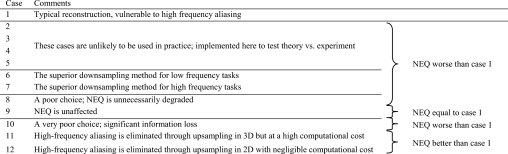
The results shown above demonstrate some of the effects of binning on the NEQ of CBCT. Cases 2–5 illustrate the major differences in the imaging performance that can be achieved on the same physical system by employing subtly different reconstructions. They confirm the accuracy of this model and demonstrate the necessity to include deterministic binning in the reconstruction cascade. Cases 6 and 7 describe the effects of downsampling to increase reconstruction speed. The results indicate that binning and downsampling in 2D before reconstruction (case 6) is favorable for low-frequency tasks, but downsampling alone (without applying an aperture) (case 7) is preferable for high-frequency tasks despite the appearance of high quantum noise; neither method performs better than a 1:1 reconstruction (case 1). In cases 8 and 9, it was demonstrated that slice averaging can be performed without affecting the NEQ, so long as the sampling interval is not increased. In cases 10–12, methods for reducing the aliased noise introduced in the reconstruction process are examined, and one is suggested (case 12) that has the opportunity to improve the image quality without significantly increasing reconstruction time. The advantages and disadvantages associated with each binning∕sampling scheme are summarized in Table 5.
Table 5.
Summary of findings related to each case of binning examined. See also Table 4.
 |
|||
|---|---|---|---|
The cases examined above are a small subset of operations that are typically performed in reconstructing and visualizing 3D data. The two-step modular binning process, as suggested here, has the flexibility to describe a range of other processes, including various interpolation schemes (for example, A=1, B=0.5, describes nearest-neighbor interpolation) and the effect of slice extraction (for example, A=1, B=infinity describes the extraction of a single slice), under a common framework, rather than special cases (e.g., as in Refs. 28, 36). The simple rectangular apertures considered here can be further extended to describe a wide range of filtering and sampling operations, providing the flexibility to tune the NEQ to a specific imaging task under a set of constraints (such as those imposed by acquisition, reconstruction, or visualization hardware and software, or simply by workflow). In the context of task-specific imaging, the ability to optimize the NEQ at certain frequencies (although at the possible expense of others) through binning is essential for the selection of knowledgeable reconstruction techniques. In some cases, the effect of various reconstruction∕binning parameters on NEQ is relatively small; in others, the effect is significant and fairly complex. The ability to analyze acquisition and reconstruction techniques within a common analytical framework, and in a manner that may be tuned to specific imaging tasks, is an important step in understanding fairly complex relationships among fundamental factors governing image quality, optimizing CBCT system performance, and ultimately translating imaging systems that provide sufficient image quality within real constraints of radiation dose and image acquisition∕reconstruction speed.
ACKNOWLEDGMENTS
The authors extend sincere thanks to Ms. Grace J. Gang (University of Toronto, Toronto, ON) for discussions relating to 3D imaging performance and to Dr. Doug Moseley, Mr. Graham Wilson, and Mr. Steve Ansell (Princess Margaret Hospital, Toronto, ON) for assistance with hardware and software aspects of the 3D imaging bench. This work was supported by National Institutes of Health Grant No. R01-CA-127944-02.
References
- Siewerdsen J. H., Cunningham I. A., and Jaffray D. A., “A framework for noise-power spectrum analysis of multidimensional images,” Med. Phys. 29(11), 2655–2671 (2002). 10.1118/1.1513158 [DOI] [PubMed] [Google Scholar]
- Fujita H., Tsai D., Itoh T., Doi K., Morishita J., Ueda K., and Ohtsuka A., “A simple method for determining the modulation transfer function in digital radiography,” IEEE Trans. Med. Imaging 11(1), 34–39 (1992). 10.1109/42.126908 [DOI] [PubMed] [Google Scholar]
- Rabbani M., Shaw R., and Van Metter R., “Detective quantum efficiency of imaging systems with amplifying and scattering mechanisms,” J. Opt. Soc. Am. A 4(5), 895–901 (1987). 10.1364/JOSAA.4.000895 [DOI] [PubMed] [Google Scholar]
- Cunningham I. A., Westmore M. S., and Fenster A., “A spatial-frequency dependent quantum accounting diagram and detective quantum efficiency model of signal and noise propagation in cascaded imaging systems,” Med. Phys. 21(3), 417–427 (1994). 10.1118/1.597401 [DOI] [PubMed] [Google Scholar]
- Yao J. and Cunningham I. A., “Parallel cascades: New ways to describe noise transfer in medical imaging systems,” Med. Phys. 28(10), 2020–2038 (2001). 10.1118/1.1405842 [DOI] [PubMed] [Google Scholar]
- Siewerdsen J. H., Antonuk L. E., El Mohri Y., Yorkston J., Huang W., Boudry J. M., and Cunningham I. A., “Empirical and theoretical investigation of the noise performance of indirect detection, active matrix flat-panel imagers (AMFPIs) for diagnostic radiology,” Med. Phys. 24(1), 71–89 (1997). 10.1118/1.597919 [DOI] [PubMed] [Google Scholar]
- Siewerdsen J. H., Antonuk L. E., El Mohri Y., Yorkston J., Huang W., and Cunningham I. A., “Signal, noise power spectrum, and detective quantum efficiency of indirect-detection flat-panel imagers for diagnostic radiology,” Med. Phys. 25(5), 614–628 (1998). 10.1118/1.598243 [DOI] [PubMed] [Google Scholar]
- Zhao W. and Rowlands J. A., “Digital radiology using active matrix readout of amorphous selenium: Theoretical analysis of detective quantum efficiency,” Med. Phys. 24(12), 1819–1833 (1997). 10.1118/1.598097 [DOI] [PubMed] [Google Scholar]
- Zhao W., Ji W. G., and Rowlands J. A., “Effects of characteristic x rays on the noise power spectra and detective quantum efficiency of photoconductive x-ray detectors,” Med. Phys. 28(10), 2039–2049 (2001). 10.1118/1.1405845 [DOI] [PubMed] [Google Scholar]
- Vedantham S., Karellas A., Suryanarayanan S., Albagli D., Han S., Tkaczyk E. J., Landberg C. E., Opsahl-Ong B., Granfors P. R., Levis I., D’Orsi C. J., and Hendrick R. E., “Full breast digital mammography with an amorphous silicon-based flat panel detector: Physical characteristics of a clinical prototype,” Med. Phys. 27(3), 558–567 (2000). 10.1118/1.598895 [DOI] [PMC free article] [PubMed] [Google Scholar]
- Vedantham S., Karellas A., and Suryanarayanan S., “Solid-state fluoroscopic imager for high-resolution angiography: Parallel-cascaded linear systems analysis,” Med. Phys. 31(5), 1258–1268 (2004). 10.1118/1.1689014 [DOI] [PMC free article] [PubMed] [Google Scholar]
- Ganguly A., Rudin S., Bednarek D. R., and Hoffmann K. R., “Micro-angiography for neurovascular imaging. II. Cascade model analysis,” Med. Phys. 30(11), 3029–3039 (2003). 10.1118/1.1617550 [DOI] [PubMed] [Google Scholar]
- Bissonnette J. P., Cunningham I. A., and Munro P., “Optimal phosphor thickness for portal imaging,” Med. Phys. 24(6), 803–814 (1997). 10.1118/1.598002 [DOI] [PubMed] [Google Scholar]
- Bissonnette J. P., Cunningham I. A., Jaffray D. A., Fenster A., and Munro P., “A quantum accounting and detective quantum efficiency analysis for video-based portal imaging,” Med. Phys. 24(6), 815–826 (1997). 10.1118/1.598009 [DOI] [PubMed] [Google Scholar]
- Drake D. G., Jaffray D. A., and Wong J. W., “Characterization of a fluoroscopic imaging system for kV and MV radiography,” Med. Phys. 27(5), 898–905 (2000). 10.1118/1.598955 [DOI] [PubMed] [Google Scholar]
- Lachaine M., “Detective quantum efficiency of a direct-detection active matrix flat panel imager at megavoltage energies,” Med. Phys. 28(7), 1364–1372 (2001). 10.1118/1.1380213 [DOI] [PubMed] [Google Scholar]
- Richard S. and Siewerdsen J. H., “Optimization of dual-energy imaging systems using generalized NEQ and imaging task,” Med. Phys. 34(1), 127–139 (2007). 10.1118/1.2400620 [DOI] [PubMed] [Google Scholar]
- Siewerdsen J. H. and Jaffray D. A., “Cone-beam CT with a flat-panel imager: Noise considerations for fully 3D computed tomography,” Proc. SPIE Physics of Medical Imaging 3977, 408–416 (2000). 10.1117/12.384515 [DOI] [Google Scholar]
- Siewerdsen J. H. and Jaffray D. A., “Unified iso-SNR approach to task-directed imaging in flat-panel cone-beam CT,” Proc. SPIE Physics of Medical Imaging 4682, 245–254 (2002). 10.1117/12.465565 [DOI] [Google Scholar]
- Siewerdsen J. H. and Jaffray D. A., “Three-dimensional NEQ transfer characteristics of volume CT using direct and indirect-detection flat-panel imagers,” Proc. SPIE Physics of Medical Imaging 29(11), 2655–2671 (2003). [Google Scholar]
- Siewerdsen J. H., Moseley D. J., and Jaffray D. A., “Incorporation of task in 3D Imaging performance evaluation: The impact of asymmetric NPS on detectability,” Proc. SPIE Physics of Medical Imaging 5368, 89–97 (2004). 10.1117/12.535744 [DOI] [Google Scholar]
- Tward D. J., Siewerdsen J. H., Fahrig R., and Pineda A. R., “Cascaded systems analysis of the 3D NEQ for cone-beam CT and tomosynthesis,” Proc. SPIE Physics of Medical Imaging 6193, 61931S-1–61931S-12 (2008). [Google Scholar]
- Tward D. J. and Siewerdsen J. H., “Cascaded systems analysis of the 3D noise transfer characteristics of flat-panel cone-beam CT,” Med. Phys. 35(12), 5510–5529 (2008). 10.1118/1.3002414 [DOI] [PMC free article] [PubMed] [Google Scholar]
- Yang K., Kwan A., Huang S., Packard N., and Boone J. M., “Noise power properties of a cone-beam CT system for breast cancer detection,” Med. Phys. 35(12), 5317–5327 (2008). 10.1118/1.3002411 [DOI] [PMC free article] [PubMed] [Google Scholar]
- Zhao B. and Zhao W., “Three-dimensional linear system analysis for breast tomosynthesis,” Med. Phys. 35(12), 5219–5232 (2008). 10.1118/1.2996014 [DOI] [PMC free article] [PubMed] [Google Scholar]
- ICRU Report No. 54, 1996. (unpublished).
- Richard S., Siewerdsen J. H., Jaffray D., Moseley D. J., and Bakhtiar B., “Generalized DQE analysis of radiographic and dual-energy imaging using flat-panel detectors,” Med. Phys. 32, 1397–1413 (2005). 10.1118/1.1901203 [DOI] [PubMed] [Google Scholar]
- Kijewski M. F. and Judy P. F., “The noise power spectrum of CT images,” Phys. Med. Biol. 32(5), 565–575 (1987). 10.1088/0031-9155/32/5/003 [DOI] [PubMed] [Google Scholar]
- Albert M. and Maidment A. D., “Linear response theory for detectors consisting of discrete arrays,” Med. Phys. 27(10), 2417–2434 (2000). 10.1118/1.1286592 [DOI] [PubMed] [Google Scholar]
- Baek J. and Pelc N. J., “Analytical construction of 3D NPS for a cone beam CT system,” Proc. SPIE Physics of Medical Imaging 7258, 725805-1–7 (2009). 10.1117/12.813832 [DOI] [Google Scholar]
- Pineda A. R., Siewerdsen J. H., and Tward D., “Analysis of image noise in 3D cone-beam CT: Spatial and Fourier domain approaches under conditions of varying stationarity,” Proc. SPIE Physics of Medical Imaging 6913, 69131Q-1–10 (2008). 10.1117/12.772966 [DOI] [Google Scholar]
- Hanson K. M., “Detectability in computed tomographic images,” Med. Phys. 6(5), 441–451 (1979). 10.1118/1.594534 [DOI] [PubMed] [Google Scholar]
- Daly M. J., Siewerdsen J. H., Moseley D. J., Jaffray D. A., and Irish J. C., “Intraoperative cone-beam CT for guidance of head and neck surgery: Assessment of dose and image quality using a C-arm prototype,” Med. Phys. 33(10), 3767–3780 (2006). 10.1118/1.2349687 [DOI] [PubMed] [Google Scholar]
- Feldkamp L. A., Davis L. C., and Kress J. W., “Practical cone-beam algorithm,” J. Opt. Soc. Am. A 1, 612–619 (1984). 10.1364/JOSAA.1.000612 [DOI] [Google Scholar]
- Siewerdsen J. H., Waese A. M., Moseley D. J., Richard S., and Jaffray D. A., “Spektr: A computational tool for x-ray spectral analysis and imaging system optimization,” Med. Phys. 31(11), 3057–3067 (2004). 10.1118/1.1758350 [DOI] [PubMed] [Google Scholar]
- Metheany K., Abbey C. K., and Boone J. M., “Characterizing anatomical variability in breast CT images,” Med. Phys. 35(10), 4685–4694 (2008). 10.1118/1.2977772 [DOI] [PMC free article] [PubMed] [Google Scholar]