A Fast Variational Method for the Construction of Resolution Adaptive C²-Smooth Molecular Surfaces

Abstract

We present a variational approach to smooth molecular (proteins, nucleic acids) surface constructions, starting from atomic coordinates, as available from the protein and nucleic-acid data banks. Molecular dynamics (MD) simulations traditionally used in understanding protein and nucleic-acid folding processes, are based on molecular force fields, and require smooth models of these molecular surfaces. To accelerate MD simulations, a popular methodology is to employ coarse grained molecular models, which represent clusters of atoms with similar physical properties by psuedo- atoms, resulting in coarser resolution molecular surfaces. We consider generation of these mixed-resolution or adaptive molecular surfaces. Our approach starts from deriving a general form second order geometric partial differential equation in the level-set formulation, by minimizing a first order energy functional which additionally includes a regularization term to minimize the occurrence of chemically infeasible molecular surface pockets or tunnel-like artifacts. To achieve even higher computational efficiency, a fast cubic B-spline C² interpolation algorithm is also utilized. A narrow band, tri-cubic B-spline level-set method is then used to provide C² smooth and resolution adaptive molecular surfaces.

1 Introduction

Molecules such as proteins and nucleic acids gain their stable configuration in solvent, which is predominantly water. Molecular dynamics (MD) simulations generate molecular motion trajectories governed by the dynamic configurations of the charged atomic entities under positionally dependent bonded and non-bonded forces. Molecules of interest for which the dynamics of folding or assembly is still unknown, range from several thousands to a few million atoms. Even in today's age of supercomputers, computing MD remains a prohibitively time and memory intensive computation, especially in explicit simulation models (where the solvent is expressed as a sufficiently large set of water molecules, surrounding the primary molecule) and to a lesser extent in the implicit simulation model (where the solvent is treated as a continuum concentration or density). Implicit MD simulations in solvent are traditionally used in understanding protein and nucleic-acid folding processes in their nativity, and based on molecular-solvent interaction force fields, require derivative continuous (smooth) models of the molecular surfaces. To accelerate MD simulations, a popular methodology is to additionally employ coarse grained molecular models, which represent clusters of atoms with similar physical properties by psuedo-atoms, resulting in coarser resolution molecular surfaces. We consider generation of these mixed-resolution or adaptive molecular surfaces.

Molecular surfaces could be represented analytically as a patch complex of spheres and tori [14] or as a patch complex of spheres and quadratic hyperboloids [19] or as parametric B-spline or NURBs [4, 5] or as level sets of summation of Gaussian atomic electron density functions [11, 12, 17, 22, 28] or implicit algebraic splines or A-patches [32]. Of course, linear surface meshes could be constructed from the analytical form [1, 13, 15, 24, 27, 31]. Simplex subdivision schemes are used to generate conforming tetrahedral meshes of the domain surrounding molecular structures in solving the Poisson-Boltzmann equation [10, 23] and subdivision coupled to geometric flow for quality tetrahedral and hexahedral meshes in [30, 31]. Since the molecular surface also acts as a dielectric interface for electrostatic and polarization energy and force computations (see [10, 21, 9]), the molecular surface should be at least C¹ smooth and not too inflated or deflated.

In this paper we present a variational approach to C² smooth molecular surface construction starting from atomic coordinate data of biomolecules, predominantly, proteins available from the Protein Data Bank (see Fig. 1.1). In Section 2 we select an appropriate regularization to the variational PDE, so that the molecular surfaces (aka dielectric interfaces) are not as inflated as the Guassian surfaces and thereby yield molecular energetics and forces that are within the range of published experimental data. Furthermore in Section 3 by spatially and selectively clustering atoms based on their use in coarse grained MD, we can additionally generate coarser resolution smooth molecular surfaces and even mixed resolution or adaptive resolution molecular surfaces (see Fig 1.2).

Fig 1.1.

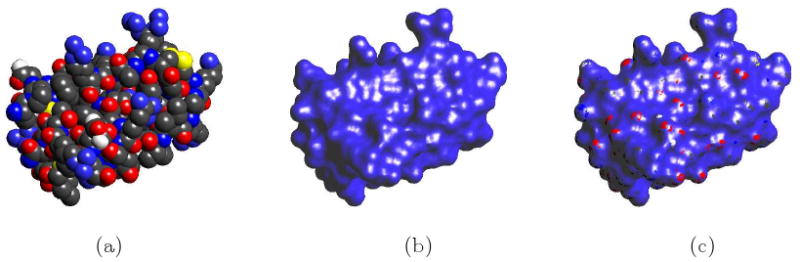
Molecular Surfaces of Protein (PDB Id: 6PTI). (a) the van der Waals surface. (b) shows our C² smooth implicit B-spline molecular surface. (c) shows the tight enclosure of the implicit B-spline molecular surface superimposed with the van der Waals surface.

Fig 1.2.

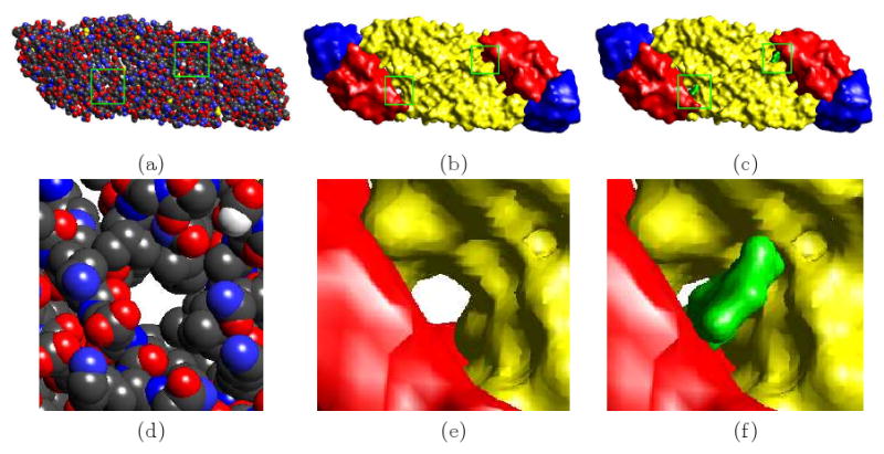
Resolution adaptive molecular surfaces of the E - Glycoprotein (PDB Id: 1OKE) of the envelope of the Dengue virus. (a) the van der Waals surface. (b) our C² implicit B-spline molecular surface of 1OKE at 10 Å resolution (Residues 1-52, 133-193 and 281-296 are colored red. Residues 53-132 and 194-280 are colored yellow. Residues 297-394 are colored blue. The coloring method is based on [25]). (c) our C² implicit B-spline molecular surface complexed with a ligand (green) at 10 Å resolution. (d) (e) and (f) are a zoomed view of the boxed portions in (a), (b) and (c) respectively (only one of the two boxes are shown in each case as they are identical).

2 Geometric Flow for Molecular Surface Construction

Given a non-negative function f(x) over a domain Ω ∈ ℝ³, we generate a molecular surface Γ in Ω, such that the energy functional

$$E(\Gamma )={\int }_{\Gamma }f(\text{x})d\text{x}+\lambda {\int }_{\Gamma }h(\text{x},\text{n})d\text{x}$$ (2.1)

is minimal, where x and n are the surface point and surface normal, respectively. h(x, n) is another given non-negative function over ℝ³ × ℝ³ which is used for regularizing the molecular surface. Here λ ≥ 0 is a constant. From minimizing energy functional (2.1), the partial differential equation (PDE) in the level-set form is obtained as the Euler Lagrange equation [7]. Furthermore an evolutionary PDE equation is obtained as an iterative (time dependent) geometric flow approximation to the PDE.

Given a molecular representation (i.e., PDB) which consists of a sequence of atoms with centers ${\left\{{\text{x}}_i\right\}}_{i=1}^m$ and radii ${\left\{r_i\right\}}_{i=1}^m$ (see Fig. 1.1(a)), we construct molecular surfaces which minimize the general energy functional (2.1). In [8], we select f(x) = g(x)² and h(x, n) = 1 with

$$g(\text{x})=1-\sum _{i=1}^m{e}^{-C_i({\Vert \text{x}-{\text{x}}_i\Vert }^2-{\stackrel{\sim }{r}}_i^2)},{\stackrel{\sim }{r}}_i=r_i+r_b,$$

where r_b is the probe radius, which usually is 1.4 Å (the radius of water). The constant C_i > 0, which is also called the Gaussian decay rate, is determined so that g(x) = 0 is an approximation of the solvent accessible surface within a given tolerance ε. We choose C_i as $\frac{\text{ln}2}{\epsilon {\stackrel{\sim }{r}}_i}$. The second term of (2.1) is used to regularize the constructed surface, where λ is a small number. In the examples provided in the following, we choose λ as 0.01. To further eliminate depression and smooth out high curavtures, we select function h(x, n) = ‖∇g(x)‖² in this paper and demonstrate its efficiency by comparing it to a number of prior analytic surfaces [6, 31]. Minimizing energy functional (2.1) for this choice of h(x, n) yields the following Euler-Lagrange equation

$$(g^2+\lambda {\Vert \nabla g\Vert }^2)\text{div}\left(\frac{\nabla \phi }{\Vert \nabla \phi \Vert }\right)+\frac{2g(\nabla g{)}^T\nabla \phi +\lambda [\nabla ({\Vert \nabla g\Vert }^2){]}^T\nabla \phi }{\Vert \nabla \phi \Vert }=0.$$

Thus the corresponding level-set formulation of the evolution equation (see [29] for derivation details or [20]) is

$$\begin{array}{l}\frac{\partial \phi }{\partial t}=(g^2+\lambda {\Vert \nabla g\Vert }^2)\text{div}\left(\frac{\nabla \phi }{\Vert \nabla \phi \Vert }\right)\Vert \nabla \phi \Vert +2g(\nabla g{)}^T\nabla \phi +\lambda [\nabla ({\Vert \nabla g\Vert }^2){]}^T\nabla \phi \\ =H(\phi )+L(\nabla \phi ),\end{array}$$ (2.2)

where

$$H(\phi )=(g^2+\lambda {\Vert \nabla g\Vert }^2)\text{div}\left(\frac{\nabla \phi }{\Vert \nabla \phi \Vert }\right)\Vert \nabla \phi \Vert ,L(\nabla \phi )=2g(\nabla g{)}^T\nabla \phi +\lambda [\nabla ({\Vert \nabla g\Vert }^2){]}^T\nabla \phi .$$

This evolution equation is solved by our higher-order level set methods [8]. The first order term L(∇φ) is computed using an upwind scheme over a finer grid, and the higher order term H(φ) is computed using a spline presentation defined on a coarser grid. If φ is a signed distance function and a steady solution of equation (2.2), then the iso-surface φ = −r_b is an approximation of molecular surface (see Fig. 1.1(b)).

We suppose that equation (2.2) is solved in a bounding box domain Ω which is uniformly partitioned with vertices $G_0={\left\{{\text{x}}_{\text{ijk}}\right\}}_{\text{ijk}=0}^n$. Let G_l be the set of vertices of the grid which is generated by binary subdivision G₀ uniformly l times. Let φ be a piecewise trilinear level set function defined on a grid G_l, with l = 0 or 1 or 2, and Φ be the cubic spline approximation of φ over grid G₀. Without loss of generality, we take l = 1 for simplicity. Thus the main algorithm in [7] can be repeated as follows.

Algorithm 1. Smooth molecular surface construction

1. Compute g(x) over the grid G_l.

2. Compute an initial φ (= φ₀) by taking φ(x) = g(x) and then update it using a reinitialization step, such that ‖∇ φ‖ = 1. Let Γ⁰ be the initial closed level set surface of φ₀ with interior ⊂ ℝ³.

3. Update φ by solving equation (2.2) for one time step using a finite difference method.

4. Reinitialize φ, convert φ to Φ, and then return to the previous step if the stopping criterion is not satisfied.

5. Generate a level set surface {x : Φ(x) = −r_b}, which is the required approximation of the smooth molecular surface.

In the following subsections, we summarize the main issues in the implementation of the above algorithm.

2.1 Level set evolution

Equation (2.2) is solved in a thin shell of the moving surface to accelerate computation and reduce errors. We first initialize φ⁰ to be the signed distance function of Γ⁰, if necessary, reinitialization step can be done first (see subsection 2.3). Then we define a thin shell around Γ⁰ by

$$N^0=\{\text{x}\in G_l:|{\phi }^0(\text{x})|<\mathscr{H}\},$$

where ℋ is the thickness of the shell should be evaluated first. To prevent numerical oscillations at the boundary of the thin shell, we should introduce a cut-off function c(x) in (2.2) as

$$\{\begin{array}{l}\frac{\partial \phi }{\partial t}=c(\phi )\left[H(\phi )+L(\nabla \phi )\right],\\ \phi (\text{x},0)={\phi }^0(\text{x}),\end{array}$$ (2.3)

on N⁰ for one time step and get φ¹(x). The time step is chosen such that the interface moves less than one grid size Δx. At each grid point x_ijk in the thin shell N⁰, compute v⁰(x_ijk) = c(φ⁰(x_ijk))[H(Φ⁰(x_ijk)) + L(∇ φ⁰(x_ijk)]. Let

$$\tau =min\left\{\Delta \text{x},\Delta \text{x}/\underset{{\text{x}}_{\text{ijk}}\in N^0}{max}|v^0({\text{x}}_{\text{ijk}})|\right\}.$$

Then update φ⁰ by the explicit Euler scheme

$${\phi }^1({\text{x}}_{\text{ijk}})={\phi }^0({\text{x}}_{\text{ijk}})+\tau v^0({\text{x}}_{\text{ijk}}),{\text{x}}_{\text{ijk}}\in N^0.$$

Since φ¹ is no longer a signed distance function, a reinitialization step is required to get a new φ¹ and a new thin shell N¹. The process from φ⁰ to φ¹ described above is repeated to get a sequence {φ^m}_m≥0 of φ, and a sequence of thin shells {N^m}_m≥0, until the following termination conditions

$$\underset{{\text{x}}_{\text{ijk}}\in N^m}{max}|v^m({\text{x}}_{\text{ijk}})|<\epsilon \text{and}m<M$$

are satisfied. We choose ε = 0.001. M is a given upper bound of the iteration number, we choose M = n, where n³ is the number of grid points in G_l.

2.2 The construction of an initial surface Γ⁰

The construction of an initial surface is pivotal to the level-set methods. If the initial surface is near to the final minimal surface, a few evolution steps are enough. In our variational molecular surface construction, we use g(x) = 0 as an initial surface Γ⁰. To further speed the computation, we use a local fast computation of the Gaussian function $e^{-C[{\Vert \text{x}-{\text{x}}_i\Vert }^2-{\stackrel{\sim }{r}}_i^2]}$ in g(x) around x_i. For details on fast Gaussian summation, refer to [6, 9].

2.3 Adaptive reinitialization

In general, it is impossible to prevent the evolving level set function φ(x) from deviating away from a signed distance function. Flat or steep regions could develop around the interface, making further computation and level set determination highly inaccurate. Hence a reinitialization step to reset the level set function φ to be a signed distance function is usually necessary. This problem has been carefully studied in [26]. The main idea is to solve a Hamilton-Jacobi equation. We omit the details here and refer the reader to [7].

3 Illustrative Examples

In this section, we provide implementation details of several applications of the methods. Our variational molecular surface algorithm has been implemented in our molecular visualization software package TexMol [2]. We now present illustrative examples of variational molecular surfaces, such as multiresolution molecular models and hierarchical macromolecular structure surfaces. Quantitative comparative surface analysis with Gaussian and adaptive grid molecular surfaces methods are also described.

3.1 Adaptive resolutions of molecular surface models

To capture molecular features, such as pockets and tunnels, one can model molecular surfaces with varying and adaptive resolution. Our variational molecular surface method provides an approach to achieve this. Since the initial surface is an approximation surface, one can select a spatially adaptive decay rate C to capture the initial surface at adaptive resolution. In Fig. 1.2, we show such an example of a ligand-binding pocket in the dengue virus (DV) envelope (E) Glycoprotein. Fig. 3.1 shows another example, where different portions of the molecular surface of a monomer of the intact human Immunoglobulin B12 (PDB Id 1HZH) are shown at different resolutions.

Fig 3.1.

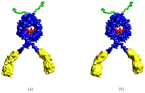
Adaptive Resolution C² Smooth Implicit B-spline Molecular Surfaces. (a) yellow legs and green antenna at about 5 Å resolution, and the blue body at about 10 Å resolution of 1HZH (PDB Id). (b) adaptive resolution with legs and antenna at about 10 Å resolution, and the body at about 5 Å resolution.

3.2 Hierarchical molecular surface segmentation of large macro-molecular complexes

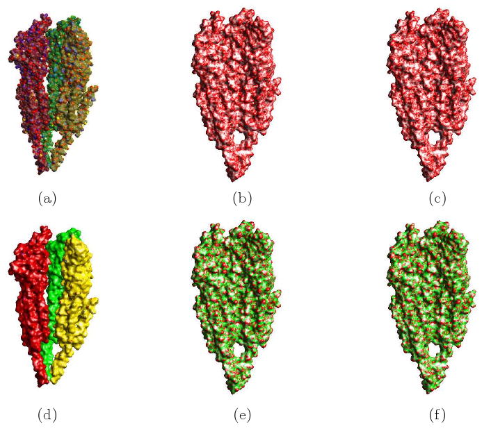
Large biomolecular complexes, such as ribosomes and viruses are assemblies of multiple proteins and nucleic acids and dozens to thousands of structural/functional biomolecular subunits. Hierarchical molecular surface segmentation with distinguishable coloring is extremely useful in achieving better understanding of the structural organization of such assemblies. Here we present one example of a hierarchical structure organization of the molecular surface of the icosahedral envelope of the Dengue Virus in Fig. 3.2. Where figure (a) is the molecular surface of two chains. Figure (b) is a molecular surface of a three-fold part of the envelope with the other parts as van der Waals surfaces. Figure (c) is a molecular surface of a five-fold part of the envelope with the other parts as van der Waals surfaces. In figure (d), molecular surfaces of different residues groups are colored differently. The other two figures are similar to (b) and (c) separately.

Fig 3.2.

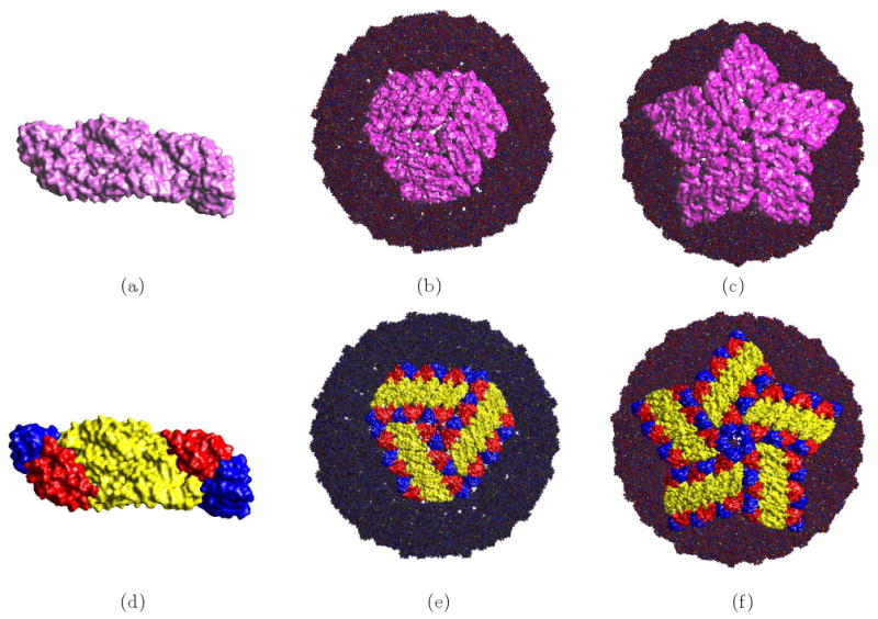
Hierarchical C²-Smooth Implicit B-Spline Molecular Surface Models of the Envelope of the Dengue Virus Figure. (a) Two chains of the monomeric envelope glycoprotein. (b) 1 three-fold envelope and the van der Waal of the other part of the envelope. (PDB Id: 1K4R) (c) 1 five-fold envelope and the van der Waal of the remain part of the envelope. (PDB Id: 1K4R). (d) the smooth implicit B-Spline molecular surface of two chains of the monomeric envelope glycoprotein colored using [25]. (e) similar to (b) using the coloring of (d). (f) similar to (b) using the coloring of (d).

3.3 Comparative examples

In this subsection, we compare our C² smooth B-spline molecular surface with molecular surfaces generated by level sets of Gaussian functions [31] and molecular surfaces generated by adaptive grid methods [6]. We also compare the difference between different regularization terms in the generation of variational molecular surfaces, in particular with respect to [7, 8].

Fig. 3.3 shows this comparison for Acetylcholinesterase complexed with Fasciculin-II, having 1FSS as its PDB Id. The molecular surface using Gaussian functions is defined by {x ∈ ℝ³ : g(x) = 1}, where $g(\text{x})={\sum }_{i=1}^n{e}^{-\frac{d}{r_i^2}\left[{\Vert \text{x}-{\text{x}}_i\Vert }^2-{\left(r_i\right)}^2\right]}$. In figure (a), we show Gaussian molecular surface. Figures (b) and (c) show the results of the adaptive grid method and our variational method. The differences between the Gaussian molecular surface with the surfaces generated by the adaptive grid method and our variational method are also respectively plotted as color mapped functions on the Gaussian surfaces. For two surfaces S₁, S₂, we calculated the difference by the following simple method

Fig 3.3.

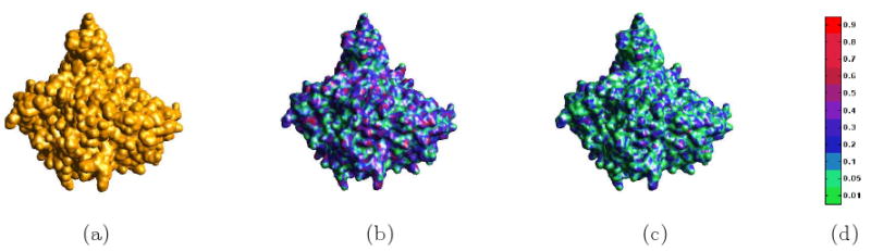
Comparison of Three Different Molecular Surface Models (PDB Id: 1FSS). (a) the Gaussian molecular surface. (b) molecular surface by the adaptive grid method with the difference between this surface and the surface of (a), displayed as a color mapped function on surface. (c) our C² molecular surface and the difference between this surface and the surface of (a), again displayed as color mapped function on surface. (d) is the color bar of the difference.

$$\text{Diff}(x,S_{\text{2}})=\text{ min}\{\text{dist}(x,y),y\in S_{\text{2}}\},x\in S_{\text{1}},$$

where dist(x,y) is the Euclidean distance of two points. Then we displayed the difference by a color mapped function defined on the initial surface S₁. In this example, we select Gaussian surface as S₂ and adaptive grid surface and our variational surface as S₁. In Fig. 3.4, an illustrative example is given for the Aspartate Carbamoyltransferase (PDB Id 4AT1). We show our molecular surface in figure (a). Similar to the above example, we depict in figure (b) the difference between our variational molecular surface and the Gaussian surface, S₂ is the molecular surface produced by our variational method. Similarly in figure (c), we show the difference between the adaptive grid molecular surface with our molecular surface. From these figures, we can see that the variational molecular surface is different from the Gaussian and adaptive grid surface.

Fig 3.4.

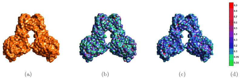
Comparison of Three Different Molecular Surface Models of the Aspartate Carbamoyltransferase (PDB Id: 4AT1). (a) our B-spline molecular surface. (b) Gaussian molecular surface with difference with (a) shown a color mapped function on surface. (c) molecular surface using an adaptive grid with grid resolution 128³ and with difference with (a) shown as a color mapped function on surface. (d) is the color bar.

To better quantitate this difference, in Table 3.1 and Table 3.2, we compare the results of area and volume computation using our variational method, and that of Gaussian, of adaptive grid molecular surfaces. The results of Gaussian molecular surfaces and adaptive grid molecular surfaces are implemented in TexMol. Since the surfaces produced by Gaussian functions often yield artifacts such as narrow depressions or tunnels and furthermore are quite inflated [3] (see Fig. 3.3 and 3.4), the surface area is enlarged and the enclosed volume is smaller. The result shows that our method gives larger volumes to Gaussian molecular surfaces but much smaller surfaces areas. They are also free from the topological surface artifacts. Comparing results with the adaptive grid method, we find that both the surface areas and volumes of our method are larger.

Table 3.1.

Surface area of different proteins computed using three different methods. A1 is computed for Gaussian molecular surface. A2 is computed for adaptive grid molecular surface. A3 is computed for the molecular surface using our methods.

Molecule	PDB Id	A1	A2	A3
Acetylcholinesterase Fasciculin	1FSS	25638.6	20233.6	20335.6
Fas.2 Mouse Acetylcholinesterase Complex	1MAH	16920.2	17061.0	17121.8
Glutamine Synthetase	2GLS	262196.6	172746.3	158346.8
Aspartate Carbamoyltransferase	4AT1	45059.5	32608.0	32300.5
HIV Capsid C	1A8O	11294.4	7015.9	6334.3
GroEL-GroES Complex	1AON	404391.4	283704.5	204322.9
Quinoprotein Methylamine Dehydrogenase	2BBK	63868.9	25349.6	21396.8
Scapharca Inaequivalvis	2Z8A	22827.4	11228.7	9997.8

Table 3.2.

Molecular volume of different proteins computed using three different methods. V1 is computed via Gaussian molecular surface. V2 is computed for adaptive grid method surface. V3 is computed for the molecular surface using our methods.

Molecule	PDB Id	V1	V2	V3
Acetylcholinesterase Fasciculin	1FSS	94653.5	78017.2	84453.0
Fas.2 Mouse Acetylcholinesterase Complex	1MAH	116586.9	113528.9	119776.8
Glutamine Synthetase	2GLS	48724.5	46250.6	42617.0
Aspartate Carbamoyltransferase	4AT1	96081.7	90061.6	97158.3
HIV Capsid C	1A8O	22997.3	21801.2	24718.3
GroEL-GroES Complex	1AON	43316.1	38817.6	30928.9
Quinoprotein Methylamine Dehydrogenase	2BBK	130205.1	133399.8	144046.2
Scapharca Inaequivalvis	2Z8A	44518.0	45002.0	50330.7

3.4 On comparison between different regularization terms

In this paper, we use another regularization term to decrease unwanted surface depression or narrow tunnel artifacts on the molecular surface. Compared with the regularization term we used in [8], while no obvious visual differences can be observed, we show example of the molecular surfaces with our different regularization term in Fig. 3.5. Figures (a) and (d) are the variational molecular surface enclosing the van der Waals surface. Figures (b) and (e) are the mean curvature and Gaussian curvature plots of the functional with area as regularization term. Figures (c) and (f) are the mean curvature and Gaussian curvature plots of the functional with the new regularization term used in this paper.

Fig 3.5.

Feature Preserving Adaptive Resolution Molecular Surfaces of the Nicotonic Acetyl-Choline Receptor Protein 2BG9. (a) (d) our molecular surface enclosing the the van der Waals surface. (b) and (c) are the mean curvature plots of the variational molecular surface generated by the minimal area regularization and the gradient magnitude squares regularization functional. (e) and (f) are the respective Gaussian curvature plots.

4 Conclusions

We have presented a general variational framework using tricubic B-spline level-set methods for C² smooth molecular surfaces. Of course, the same technique can yield surfaces of higher continuity, if so desired by the application. We additionally compared our molecular surfaces with molecular surfaces obtained by taking a level set of Gaussian functions, and note that our new variational method yields much more smoother and tighter molecular surfaces, (relevant for more accurate electrostatic potentials and energetics calculations when the molecular surfaces are used as dielectric interfaces), relative to several prior popular molecular surface generation techniques. Compared with adaptive grid molecular surface, our results have more appropriate surface area and molecular volume. Our variational molecular surface method can additionally be used to produce multiresolution molecular models and hierarchical interfaces of large molecular complexes. Although we experienced with a new regularization, the results obtained were not substantially different. Thus a good regularization function is an area of further research [18].

References

- 1.Akkiraju N, Edelsbrunner H. Triangulating the surface of a molecule. Discr Appl Math. 1996;71:5–22. [Google Scholar]
- 2.Bajaj C, Djeu P, Siddavanahalli V, Thane A. Texmol: interactive visual exploration of large flexible multi-component molecular complexes. VIS'04: Proceedings of the conference on Visualization '04; Washington, DC, USA. 2004. pp. 243–250. [Google Scholar]
- 3.Bajaj C, Gillette A, Goswami S. Topology based selection and curation of level sets. In: Wiebel A, Hege H, Polthier K, Scheuermann G, editors. Topology In Visualization. 2007. In Publication. [DOI] [PMC free article] [PubMed] [Google Scholar]
- 4.Bajaj C, Lee H, Merkert R, Pascucci V. NURBS based B-rep models from macromolecules and their properties. Proceedings Fourth Symposium on Solid Modeling and Applications; 1997. pp. 217–228. [Google Scholar]
- 5.Bajaj C, Pascucci V, Shamir A, Holt R, Netravali A. Dynamic maintenance and visualization of molecular surfaces. Discrete Applied Mathematics. 2003;127:23–51. [Google Scholar]
- 6.Bajaj C, Siddavanahalli V. Technical Report TR-06-56. Department of Computer Science, The University of Texas at Austin; 2006. Adaptive grid based methods for computing molecular surfaces and properties. [Google Scholar]
- 7.Bajaj C, Xu G, Zhang Q. ICES Report 06-18. Institute for Computational and Applied Mathematics, The University of Texas at Austin; 2006. Smooth surface construction via a higher order level set method. [Google Scholar]
- 8.Bajaj C, Xu G, Zhang Q. Higher-order level-set method and its application in biomolecular surfaces construction. J Comput Sci & Technol. 2008;23(6) doi: 10.1007/s11390-008-9184-1. [DOI] [PMC free article] [PubMed] [Google Scholar]
- 9.Bajaj C, Zhao W. ICES Report 08-20. Institute for Computational Engineering and Sciences, The University of Texas at Austin; 2008. Fast molecular energetics and forces computation. [Google Scholar]
- 10.Baker N, Sept D, Joseph S, Holst M, McCammon J. Proc Natl Acad Sci. Vol. 98. USA: 2001. Electrostatics of nanosystems: application to microtubules and the ribosome; pp. 10037–10041. [DOI] [PMC free article] [PubMed] [Google Scholar]
- 11.Blinn J. A generalization of algebraic surface drawing. ACM Transactions on Graphics. 1982;1(3):235–256. [Google Scholar]
- 12.Can T, Chen C, Wang Y. Efficient molecular surface generation using level-set methods. J Mol Graph Model. 2006;24(4):442–454. doi: 10.1016/j.jmgm.2006.02.012. [DOI] [PubMed] [Google Scholar]
- 13.Cheng HL, Dey T, Edelsbrunner H, Sullivan J. Dynamic skin triangulation. Discr Comput Geom. 2001;25:525–568. [Google Scholar]
- 14.Connolly M. Analytical molecular surface calculation. Journal of Applied Crystallography. 1983;16(5):548–558. [Google Scholar]
- 15.Connolly ML. Molecular surfaces: A review. 1996 http://www.netsci.org/Science/Compchem/feature14.html.
- 16.CVC. TexMol. http://ccvweb.csres.utexas.edu/ccv/projects/project.php?proID=8.
- 17.Duncan BS, Olson AJ. Shpae analysis of molecular surfaces. Biopolymers. 1993;33:231–238. doi: 10.1002/bip.360330205. [DOI] [PubMed] [Google Scholar]
- 18.Dzubiella J, Swanson JMJ, McCammon JA. Coupling hydrophobic, dispersion, and electrostatic contributions in continuum solvent models. Physical Review Letters. 2006;96(8):087802. doi: 10.1103/PhysRevLett.96.087802. [DOI] [PubMed] [Google Scholar]
- 19.Edelsbrunner H. Deformable smooth surface design. Discre & Comput Geom. 1999;21(1):87–115. [Google Scholar]
- 20.Faugeras OD, Keriven R. Variational principles, surface evolution, PDE's, level-set methods, and the stereo problem. IEEE Trans Image Process. 1998;7(3):336–344. doi: 10.1109/83.661183. [DOI] [PubMed] [Google Scholar]
- 21.Gerstein M, Richards F, Chapman M, Connolly M. International Tables for Crystallography. Crystallography of Biological Molecules. Kluwer; Dortrecht, Netherlands: 2001. Protein surfaces and volumes: measurement and use; pp. 532–545. [Google Scholar]
- 22.Grant J, Pickup B. A Gaussian description of molecular shape. Journal of Phys Chem. 1995;99:3503–3510. [Google Scholar]
- 23.Holst M, Baker N, Wang F. Adaptive multilevel finite element solution of the Poisson-Boltzmann equation i: Algorithms and examples. J Comput Chem. 2000;21:1319–1342. [Google Scholar]
- 24.Laug P, Borouchaki H. Molecular surface modeling and meshing. Engin with Computers. 2002;18:199–210. [Google Scholar]
- 25.Modis Y, Ogata S, Clements D, Harrison SC. A ligand-binding pocket in the dengue virus envelope glycoprotein. Proceedings of the National Academy of Sciences of the United States of America. 2003;100(12):6986–6991. doi: 10.1073/pnas.0832193100. [DOI] [PMC free article] [PubMed] [Google Scholar]
- 26.Peng D, Merriman B, Osher S, Zhao H, Kang M. A PDE-based fast local level set method. J Comp Phy. 1999;155(2):410–438. [Google Scholar]
- 27.Varshney Amitabh, Brooks Frederick P. Fast analytical computation of richards's smooth molecular surface. IEEE Visualization '93 Proceedings. 1993:300–307. [Google Scholar]
- 28.Weiser J, Shenkin P, Still W. Optimization of Gaussian surface calculations and extension to solvent-acccessible surface areas. J Comput Chem. 1999;20(7):688–703. doi: 10.1002/(SICI)1096-987X(199905)20:7<688::AID-JCC4>3.0.CO;2-F. [DOI] [PubMed] [Google Scholar]
- 29.Xu G, Zhang Q. Construction of geometric partial differential equations in computational geometry. Mathematica Numerica Sinica. 2006;28(4):337–356. [Google Scholar]
- 30.Zhang Y, Bajaj C, Xu G. Surfaces smoothing and quality improvement of quadrilateral/hexahedral meshes with geometric flow. Proc of 14th International Meshing Roundtable; San Diego, CA. September 11-14, 2005.pp. 449–468. [Google Scholar]
- 31.Zhang Y, Xu G, Bajaj C. Quality meshing of implicit solvation models of biomolecular structures. Computer Aided Geometric Design. 2006;23(6):510–530. doi: 10.1016/j.cagd.2006.01.008. [DOI] [PMC free article] [PubMed] [Google Scholar]
- 32.Zhao W, Xu G, Bajaj C. An algebraic spline model of molecular surfaces. Proceedings of the 2007 ACM symposium on Solid and physical modeling; Beijing, China. 2007; IEEE; pp. 297–302. [Google Scholar]