Transport of Relational Structures in Groups of Diffeomorphisms

Abstract

This paper focuses on the issue of translating the relative variation of one shape with respect to another in a template centered representation. The context is the theory of Diffeomorphic Pattern Matching which provides a representation of the space of shapes of objects, including images and point sets, as an infinite dimensional Riemannian manifold which is acted upon by groups of diffeomorphisms. We discuss two main options for achieving our goal; the first one is the parallel translation, based on the Riemannian metric; the second one, based on the group action, is the coadjoint transport. These methods are illustrated with 3D experiments.

1 Introduction

There is a large amount of work on template-centered shape analysis. The point of view for this is to describe shape variations across subjects based on a normalized representation, obtained by aligning the subjects to a template, allowing for reliable statistical analyses [3, 4, 6, 12–14, 23–25, 27, 29–31].

In this paper, we consider the issue of transporting relations between shapes, or images from a subject-dependent representation to a single template. The application context is as follows. Assume that we observe longitudinal data, time series or group data. We can locally analyze the within-subject or within-group variations, independently for each group, and therefore independently from any between-subject variation. Once this analysis is done, and some statistical description of the shape distribution for each group is obtained, the next step should be to collect these descriptors in a common reference system, where everything is aligned with a template. For this, the alignment process must not only transport shapes, but also the information that describes the within-group variations.

The present paper is an attempt to formalize a rigorous and computational approach to this problem in the context of the theory of Diffeomorphic Pattern Matching, developed in particular in [4, 6, 11, 33]. We will develop the mathematical machinery and provide some preliminary illustrations of the method. The first one uses triangulated surfaces, and provides an assessment of the asymetry of the hippocampus in the left and right parts of the brain. We will compute relative deformations from left to right hippocampi, then transport them to a single template to analyze their structure in a common “coordinate system”. The other experiment deals with paired data (twins). Our goal, here, is to illustrate what could constitute an averaged deformation between two twins hippocampi when one of the siblings twin has been struck by a mental disease (and the other one has not). The illustration proposed here only provide descriptive results (without statistical assessments), but a study along these lines with a larger dataset is currently being developed, with the potential outcome that, while analyzing within-twin variation in this context, one would be able to describe with more reliability specific consequences of the onset of the disease that would not be caused by genetic factors. In addition to these two illustrations, another application of the proposed method can deal with the analysis of longitudinal data, for example a baseline and a follow-up image for each subject of the dataset, the goal being to describe the evolution with a representation that would be independent of the original anatomy of the subjects.

We now proceed with a discussion of Diffeomorphic Pattern Matching, [11, 33]. A primary application of this theory is the search for correspondences between two images or, more generally, the registration of a database of subjects I ₁, …, I_N to a single template I_temp. The kth subject is registered by a diffeomorphism, ϕ_k, which is estimated as an optimizer of an energy of the form [6, 11, 33] (let id be the identity function)

$$E(\mathit{\varphi })=D{(\text{id},\mathit{\varphi })}^2+\frac{1}{{\mathit{\sigma }}^2}||I_{\mathit{\text{temp}}}\circ {\mathit{\varphi }}^{-1}-I_k|{|}_2^2.$$ (1)

In this energy, I_temp ∘ ϕ⁻¹ is the template deformed by the diffeomorphism ϕ. Note that this is an approximate matching procedure: the deformed template does not exactly coincide with the target, although the error is generally small in practice.

In (1), images and diffeomorphisms are assumed to be defined on an open subset Ω of ℝ^d, and space integrals are taken over Ω. The first term in (1), D (id,ϕ)², is a squared distance between the identity transformation and ϕ. This distance is obtained by placing a Riemannian structure on the group of diffeomorphisms [22–24, 32, 34]. This will be summarized later in this section.

A similar approach can be taken replacing images with point sets or landmarks. In this situation, diffeomorphisms act on sets x̄ = (x(1), …,x(Q)) where x(q) ∈ ℝ^d,q = 1, …, Q, with

$$\mathit{\varphi }\cdot \overline{x}=(\mathit{\varphi }(x(1)),\dots ,\mathit{\varphi }(x(Q))).$$

A problem analogous to (1) can be defined as

$$E(\mathit{\varphi })=D{(\text{id},\mathit{\varphi })}^2+\frac{1}{{\mathit{\sigma }}^2}\sum _{q=1}^Q{(y(q)-\mathit{\varphi }(x(q)))}^2.$$ (2)

This is the labelled point (or landmark) matching problem, considered in this form in [18]. Other point-based matching problems have been considered, for curves and surfaces [35], and lead to similar expressions with a different data attachment term.

The advantage of such an approach is to always provide diffeomorphic (non-ambiguous) correspondences, while conserving a notable degree of smoothness, even for very large deformations. For this reason, we termed the approach as Large Deformation Diffeomorphic Metric Mapping (LDDMM). Its tradeoff is an increase of the computational complexity compared to other “static” methods [5, 7, 27, 28]. In the following, we briefly introduce the framework of LDDMM.

As introduced in [9], we build diffeomorphisms as flows associated to non-homogeneous ordinary differential equations (ODE's), of the form y_t = v(t, y). (Here and in the rest of the paper, derivatives and partial derivatives are indicated by subscripts: y_t = dy/dt.) The function v is a time-dependent vector field which becomes an auxilliary variable for the matching problem. It is assumed to vanish on the boundary of Ω (or at infinity if Ω is not bounded). It generates a time-dependent diffeomorphism (the associated flow), defined by

$$\begin{array}{cc}{\mathit{\varphi }}_t^v(t,x)=v(t,{\mathit{\varphi }}_v(t,x)),\hfill & {\mathit{\varphi }}^v(0,x)=x\hfill \end{array}$$ (3)

(again, ${\mathit{\varphi }}_t^v$ is the partial derivative of ϕ^v with respect to time). Diffeomorphisms generated in this way have been shown to form a group, i.e., their set is closed by composition and inversion of functions. Using v as an auxilliary variable leads to formulate the inexact matching problem between images I_temp and I_k, as the search for the minimum of the energy

$$\stackrel{\sim }{E}(v)={\mathit{\int }}_0^1||v(t)|{|}_v^2\mathit{\text{dt}}+\frac{1}{{\mathit{\sigma }}^2}||I_{\mathit{\text{temp}}}\circ {\mathit{\varphi }}^v{(1)}^{-1}-I_k|{|}_2^2$$ (4)

where v(t) and ϕ^v(t) are the functions x ↦ v(t, x) and x ↦ ϕ^v(t, x), and ‖.‖_V refers to a norm over vector fields that will be discussed later. This problem, formulated in [11, 33], has been numerically solved in [4, 6].

This formulation is in fact a special case of (1). This is because

$$D(\mathit{\varphi },\stackrel{\sim }{\mathit{\varphi }}):=\text{min}\left\{\sqrt{{\mathit{\int }}_0^1||v(t)|{|}_v^{2}dt}:\stackrel{\sim }{\mathit{\varphi }}={\mathit{\varphi }}^v(1)\circ \mathit{\varphi }\right\}$$

is a distance between diffeomorphisms, and min_v Ẽ(v) = min_ϕE(ϕ) with

$$\begin{array}{c}E(\mathit{\varphi })=\underset{v:{\mathit{\varphi }}^v(1)=\mathit{\varphi }}{\text{min}}\stackrel{\sim }{E}(v)\hfill \\ =D{(\text{id},\mathit{\varphi })}^2+\frac{1}{{\mathit{\sigma }}^2}||I_{\mathit{\text{temp}}}\circ {\mathit{\varphi }}^{-1}-I_k|{|}_2^2.\hfill \end{array}$$

Finally, we note that (1) and (4) can also be reformulated in terms of image distances. Indeed, define, for two images I, I′

$$D^{\ast }(I,I^{\prime })=\text{inf}\{D(\text{id},\mathit{\varphi }):I\circ {\mathit{\varphi }}^{-\text{1}}=I^{\prime }\},$$ (5)

the left-hand side being infinite if the set in the right-hand side is empty. Then, (1) and (4) are clearly equivalent to minimizing

$$E^{\ast }(J)=D^{\ast }{(I_{\mathit{\text{temp}}},J)}^2+\frac{1}{{\mathit{\sigma }}^2}{\Vert J-I_k\Vert }_2^2.$$ (6)

The metric D* is the distance induced by D on images. Similarly, one can consider an induced metric on point sets, defined by

$$D^{\ast }\left(\overline{x},{\overline{x}}^{\prime }\right)=\text{inf}\left\{D(\text{id},\mathit{\varphi }):\mathit{\varphi }.\overline{x}={\overline{x}}^{\prime }\right\}$$ (7)

and the following equivalent formulation of (2), this time between two point sets x̄_temp and x̄_k

$$E\left(\overline{z}\right)=D^{\ast }{({\overline{x}}_{\mathit{\text{temp}}},\overline{z})}^2+\frac{1}{{\mathit{\sigma }}^2}\sum _{q=1}^Q{|z(q)-x_k(q)|}^2.$$ (8)

The Euler-Lagrange equation associated to the optimization problem that needs to be solved to compute the distance D (which is in fact a Riemannian metric between diffeomorphisms) constrains the optimal v to satisfy an evolution equation, called EPDiff, which has been described in abstract form by Arnold [1, 2]. This equation, which is detailed in the next section, also derives from an application of the Euler-Poincaré principle, as described in [16, 20]. In physics, it is related to the Euler equation for compressible fluids and to the Camassa-Holm equation which models the motion of waves in shallow water [8]. A discussion of the EPDiff equation in the particular case of template matching is provided in [23], and a parallel with the solitons emerging from the Camassa-Holm equation is discussed in [17].

One important remark is that this equation can be used to reduce the number of variables with respect to which the minimization of Ẽ is performed. This is because the specification of v(0) uniquely defines a trajectory v(t) as a solution of the EPDiff equation. This implies that a solution of our minimization problem (whether in terms of ϕ or of v) is uniquely characterized by v(0). This initial velocity can therefore be used to describe and characterize the template/target relation for a database of shapes [23, 36]. One can also develop a matching algorithm designed to solve the minimization problem using only v(0) as a free parameter [37].

As already stated, we are interested, in this paper, in registering not only the shapes themselves, but some within-group relations among them. In this context, each group (or subject) is represented by a family of shapes, the data taking the form: I₁₀, …, I_1n, I₂₀, …, I_2n, …, I_N0, …, I_Nn where I_kj is the (j + 1)th observation in group k. We also assume that a “global” template is available (or estimated). We shall refer to it as the between-group template. In an approach that consists in registering all the images to the template and using a deformation signature to characterize the subjects (like the Jacobian, or the initial velocity that we have just discussed), the obtained description will incorporate both within- and between-group variations. When the latter are large, within-group variations (which are features of interest here) will appear as a second order phenomenon, and therefore be harder to analyze. It is therefore more appealing to first characterize within-group variations locally, i.e., separately for each group, and then transport the result to a common template-based representation, as summarized in Fig. 1.

Fig. 1.

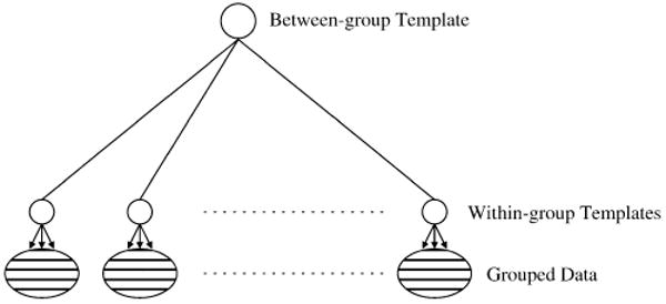
Generic relational model: the within-group templates collect the local variation within each groups. These variation are then transfered to the between-group template

Providing algorithmic tools to achieve this goal is the central subject of this paper. We shall exploit the group and metric structures of the manifold of diffeomorphisms to define translation mechanisms for within-group relations, and algorithms to compute them. We will first describe how to represent within-group relations, which will be done, as natural on a manifold, by using tangent vectors. We will then show how such vectors can be transported along the manifold, focusing on two options: parallel transport and coad-joint. We finally apply the parallel transport algorithm in preliminary experiments on cardiac and brain data.

2 Fundamental Evolution Equations on Groups of Diffeomorphisms

2.1 Notation

We will work in dimension d = 2 or 3 and assume that all images are defined on a common continuous domain Ω, which is an open subset of ℝ^d. The velocity fields (t ↦ v(t)) that drive our evolving diffeomorphisms will be assumed to belong at all times in a fixed Hilbert space v. Elements of v are assumed to be square integrable and to have enough partial derivatives that vanish on ∂Ω or at infinity (more specific conditions can be found in [11, 32–34]).

v being a Hilbert space, it has an inner product which will be denoted (v, w) ↦ 〈v, w〉_V. The continuous linear forms on v form its topological dual, v*. The evaluation of m ∈ v* at v ∈ v (i.e., m(v)) will be denoted (m | v). The duality operators K : v* → v and L = K⁻¹ : v → v* are defined by (m | v) = 〈Km, v〉_V and 〈v, w〉_V = (Lv | w). They are symmetric in the sense that (m | Kp) = (p | Km) and (Lv | w) = (Lw | v). The set v can be defined either by specifying L or K. An example of the former case is the choice a differential operator L = (−Δ + αI)^q, made, for example, in [6]. If one prefers the second option, a valid choice is a kernel operator of the form

$$Km={\mathit{\int }}_{\Omega }K(x,y)m(y)\mathit{\text{dy}},$$

with K(x, y) = exp(−|x − y|²/2σ²) (Gaussian kernel).

We will denote by G_V the group of diffeomorphisms [33] obtained by computing the flow associated to a time-dependent vector field v(t) (as defined in (3)), with v satisfying

$${\mathit{\int }}_0^1{\Vert v(t)\Vert }_v^2\mathit{\text{dt}}<\infty .$$

If A is a linear operator from v to v and has a dense range, its conjugate, A* : V* → v*, is defined by (A*m | v) = (m | Av).

2.2 The EPDiff Equation

If t ↦ ϕ(t, .) ∈ G_V is an evolving diffeomorphism that satisfies the equation ϕ_t = v(t, .) with v(t, .) ∈ v, we will call, like we did before, v(t, .) the velocity of the deformation at time t, and m(t) = Lv(t) the momentum of the deformation. The term “momentum” is justified by the fact that the energy associated to the velocity at time t in (1) is ${\Vert v(t)\Vert }_v^2$, which is also equal to (Lv(t) | v(t)), the latter expression taking the usual form of momentum applied to velocity.

The Riemannian distance defined in Introduction arises from a right invariant Riemannian metric on G_V that coincides with 〈. , .〉_V at the identity. This is a general construction which is studied in detail elsewhere [2, 16, 23, 33]. A geodesic equation in this group (starting from the identity in the direction v(0, .)) can be characterized by a beautiful conservation equation that relates to the conservation of momentum [1]. One can prove that the velocity field, v(t, .), along the geodesic (which is defined by the relation ϕ_t = v(t, ϕ)) satisfies at all times the property: for all w ∈ v

$$(Lv(t)|w)=(Lv(0)|{(D\mathit{\varphi }(t))}^{-1}w\circ \mathit{\varphi }(t)).$$ (9)

This equation uniquely specifies Lv(t) as a linear form on v, given the initial momentum and the evolving diffeomorphism ϕ(t). We will refer to it as the EPDiff equation [16].

For a diffeomorphism ϕ, the linear transformation w ↦ (Dϕ ∘ ϕ⁻¹)w ∘ ϕ⁻¹ is called the Adjoint of ϕ and denoted w ↦ Ad_ϕw. The conservation of momentum can therefore be written (Lv(t) | w) = (Lv(0) | Ad_ϕ(t)−1 w) or, by definition of a dual transformation, Lv(t) = (Ad_ϕ(t)−1)*(Lv(0)). When m(0) = Lv(0) is a function (in which case (m(0) | w) is simply given by ∫_Ωm(0)^Twdx), a change of variables provides the expression of (Ad_ψ)*m(0) which is

$${\left({\mathit{\text{Ad}}}_{\mathit{\psi }}\right)}^{\ast }m(0)={\left(D\mathit{\psi }\right)}^{T}m(0)\circ \mathit{\psi }|\text{det}D\mathit{\psi }|$$

where ψ is a diffeomorphism. Note that Lv(0) being a function is a very particular case; in general, Lv(0) belongs to v*, the dual space of v, which contains functions, but also measures and more general distributions. However, in this particular case, the conservation of momentum takes the classical form:

$$m(t)={\left(D\mathit{\psi }\right)}^{T}m(0)\circ \mathit{\psi }|\text{det}D\mathit{\psi }|\mathit{\text{with}}\mathit{\psi }=\mathit{\varphi }{(t)}^{-1}.$$

An equivalent form of EPDiff can be obtained by computing the time derivative of (9), yielding

$$\left(\frac{\mathit{\text{dLv}}(t)}{\mathit{\text{dt}}}|w\right)=-(Lv(t)|a{d}_{v(t)}w)$$ (10)

where ad_v : w ↦ Dv.w − Dw.v is the adjoint (with a small “a”) operator on v. This leads to the equation, for m = Lv:

$$\frac{\mathit{\text{dm}}}{\mathit{\text{dt}}}+a{d}_v^{\ast }m=0$$ (11)

which also has a classical expression when m is a smooth function

$$\frac{\mathit{\text{dm}}}{\mathit{\text{dt}}}+D{v}^{T}m+\mathit{\text{Dmv}}+m\text{div}v=0$$ (12)

Under some assumptions on the operator L, the system of equations

$$\{\begin{array}{l}{\mathit{\varphi }}_t=v(t,\mathit{\varphi }),\\ Lv(t)={(A{d}_{\mathit{\varphi }{(t)}^{-1}})}^{\ast }(Lv(0))\end{array}$$

has a unique solution over all times with the initial condition ϕ(0) = id, providing a time-dependent diffeomorphism that we will denote ϕ^v(0) (t). A proof of this statement can be easily deduced from [34], Theorem 7. This is the exponential map on G_V, for its right invariant Riemannian structure. The usual notation for it is

$${\mathit{\varphi }}^{v(0)}(t)={\text{Exp}}_{\text{id}}(tv(0)).$$

One interesting aspect of (9) is that it describes the evolving diffeomorphism ϕ as the solution of a first order equation in time, namely

$${\mathit{\varphi }}_t=\left(K\left({(A{d}_{\mathit{\varphi }{(t)}^{-1}})}^{\ast }(\mathit{\text{Lv}}(0))\right)\right)\circ \mathit{\varphi }.$$

As a consequence, taking ϕ(0) = id, this evolution is uniquely specified by the value of v(0) (the initial velocity) or equivalently of Lv(0), the initial momentum.

Since the minimum of (1) must satisfy (9), it is entirely specified by its initial momentum Lv(0). As suggested in [23], we can use it as a deformation signature to describe the deformed template I_temp∘ ϕ⁻¹. It must be noticed that the momentum associated to this variational problem has a simple structure that is related to the template [6, 23]. In the image matching case, it always takes the form

$$\mathit{\text{Lv}}(0)=\mathit{\alpha }\nabla I_{\mathit{\text{temp}}}=\mathit{\alpha }|\nabla I_{\mathit{\text{temp}}}|N_{\mathit{\text{temp}}}$$ (13)

where N_temp = ∇I_temp/|∇I_temp| (taking by convention N_temp = 0 if ∇ I_temp = 0) is the normal to the level sets of the template, oriented in the direction of increasing intensities. The template being fixed, the initial momentum is uniquely specified by the scalar field z = α | ∇I_temp |. The exact expression of α in terms of the optimal diffeomorphism (for target I_k) is, for problems like (4),

$${\mathit{\alpha }}_k=\frac{1}{{\mathit{\sigma }}^2}|\text{det}D{\mathit{\varphi }}_k|\left(I_{\mathit{\text{temp}}}-I_k\circ {\mathit{\varphi }}_k\right).$$

In the situation of a dataset I_temp, I₁, …, I_N, we see that the previous analysis provides a template centered representation, obtained after minimizing (1) for each I_k. This representation takes the form z₁, …,z_N with z_k = α_k|∇I_temp|.

The initial momentum is even simpler in the case of point sets. If x̄_temp is the template point set, we must have

$$\mathit{\text{Lv}}(0)=\sum _{q=1}^Q\mathit{\alpha }(q){\mathit{\delta }}_{x_{\mathit{\text{temp}}}(q)}.$$ (14)

This (singular) momentum is therefore parameterized by ᾱ = (α(1), …,α(M)), each α(q) being a d-dimensional vector.

The obtained representation can be used as a basis for statistical studies, as done in [36] for hippocampi (in the landmark matching case) or in [15] for cardiac data (in the image case). We consider, in the next section as well as in Sect. 5, some operations that transport momenta relative to a given object to momenta aligned with another object. Because of its simplicity and its practical usefulness, it is important to ensure that the specific structure of the momentum still remains valid at the end of the operation.

3 Parallel Transport for Point-Set Information

For longitudinal or group studies, the situation suggested in the introduction is as follows. The dataset (in the point-set case) takes the form x̄_temp, x̄₁₀, …, x̄_1n, x̄₂₀, …, x̄_2n, …, x̄_N0, …, x̄_Nn. As a convention, let's consider that x̄_k0 is a reference view for subject k (similar notation will be used for images). The reference view can be the image at a reference time (e.g., beginning of the study), or an average view estimated from the other ones. It is called the within-group template. The strategy we suggest to compare within-group variation in such a dataset requires to first perform a within-group registration, of each x̄_kj, j ≥ 1, to x̄_k0. As described in (14), this results, for each k, in a sequence of collection of vectors ᾱ _kj, j = 1, …, N (corresponding to the registration of x̄_kj on x̄_k0). At the end of this operation, each ᾱ _kj is associated with the within-group template, x̄_k0. In order to allow for a joint analysis of these features, we need to register them again, this time to the between-group template x̄_temp. This will be implemented with parallel translation, which is the simplest way to transport vectors in a Riemannian manifold. It will conserve the specific structure of the momentum, discussed in the previous section, as well as the norms and dot products of the transported vectors for the considered metric. We now focus on this operation, first for point sets, then for images.

Note that the initial momentum is the most general quantity that can be transported in our context. Since the initial momentum encodes the whole diffeomorphism (via the solution of (9)), transporting it implicitely transports the within-group deformations. These deformations, based on the transported momentum, can then be visualized and analyzed relatively to the between-group template, as will be illustrated in our experiments.

3.1 Parallel Translation

Parallel translation in a Riemannian manifold is performed along a curve γ traced on this manifold. If X = X(0) is a tangent vector at γ(0), the operation provides a time-dependent vector X(t) at γ(t). In principle, parallel transport is characterized by the equation ∇_γt X = 0 that involves the covariant derivative associated to the metric. In a local chart, this equation is

$${\mathit{\text{X}}}_{\mathit{\text{t}}}^{\mathit{\text{k}}}+\sum _{i,j=1}^d{\Gamma }_{ij}^k{X}^i{\mathit{\gamma }}_t^j=0$$ (15)

where ${\Gamma }_{\mathit{\text{ij}}}^{\mathit{\text{k}}}$ are the Christoffel symbols. Parallel translation ensures that X is constant along the curve according to the intrinsic geometry of the manifold.

When vectors are moved along geodesics, there is a nice interpretation of this operation in terms of perturbation of geodesics. In Euclidean geometry, when the straight line t ↦ tξ is perturbed into a new line t ↦ t(ξ + εη), the difference between their position at time t is tεη, which is, up to a renormalization, the initial perturbation η.

This obvious fact partially subsists on manifolds, in the sense that if γ(t) = Exp_γ(0) (tξ) is the geodesic starting at γ (0) in the direction ξ, and if γ^ε (t) = Exp_γ(0) (t (ξ + εη)), then, at small time δt, the little piece of curve ε ↦ γ^ε(δt)/δt is approximately oriented, at ε = 0, like the parallel translation of η along γ, and this up to an order 2 in δt. This fact, which is illustrated in Fig. 2 (see also [2]), can be formalized more rigorously as follows.

Fig. 2.

Parallel transport using iterated Jacobi fields

First, the variation of γ^ε(δt) with respect to ε at ε = 0 is captured by the derivative

$$J_{\mathit{\gamma }(0)}(t,\xi ,\mathit{\eta }):=\frac{\partial }{\partial \mathit{\epsilon }}{\text{Exp}}_{\mathit{\gamma }(0)}(t(\xi +\mathit{\epsilon }\mathit{\eta })).$$

This function, which is a perturbation of the exponential map, is a well-known object in Riemannian geometry, called a Jacobi field. It satisfies a differential equation along the geodesic, which, in full generality, is given by

$$\frac{D^{2}J}{D{t}^2}+\text{Ric}(J,{\mathit{\gamma }}_t){\mathit{\gamma }}_t=0$$ (16)

where Ric is the Ricci curvature. Here D/Dt is the covariant derivative along the geodesic. In fact, for our purpose, the only relevant facts are that J(0) = 0, DJ/Dt(0) = η and D²J/Dt² (0) = 0, three facts that imply that

$$\frac{J(\mathit{\delta }t)}{\mathit{\delta }t}-P_{\mathit{\delta }t}(\mathit{\eta })=o(\mathit{\delta }t)$$ (17)

where P_δt(η) is the parallel translation of η along γ from time t = 0 to time t = δt. Indeed, a direct computation in a chart shows that

$$\frac{d^2{J}^k}{d{t}^2}(0)=-2\sum _{\mathit{\text{ij}}=1}^d{\Gamma }_{\mathit{\text{ij}}}^k{\xi }^i{\mathit{\eta }}^j$$ (18)

yielding

$$J^k(\mathit{\delta }t)=\mathit{\delta }t{\mathit{\eta }}^k-\mathit{\delta }{t}^2\sum _{\mathit{\text{ij}}=1}^d{\Gamma }_{\mathit{\text{ij}}}^k{\xi }^i{\mathit{\eta }}^j+o(\mathit{\delta }{t}^2)$$

which directly leads to (17).

We therefore obtain a first order discretization scheme for parallel translation by iterating the computation of Jacobi fields over small intervals. This is summarized by Algorithm 1.

Of course, Algorithm 1 is useful only if the function J can be computed efficiently. We now provide these equations for point sets, and then subsequently for images and for groups of diffeomorphisms, which will complete Algorithm 1. Also, the obtained complexity can be compared with a direct implementation of equation (15) when it is available.

Algorithm 1 Discretized parallel translation along a geodesic using iterated Jacobi fields

0. Initialize variables: ξ, η, x.

for t = 1 to T do

1.1 Compute the geodesic starting at x in the direction ξ.

Let x0 be its position at time δt = 1/T and ξ0 its velocity at the same time.

1.2 Compute η0 = T Jx (1/T, ξ, η).

1.3 Set x ← x0, ξ ← ξ0 and η ← η0.

end for

3.2 Transporting Point-Set Information

We now apply the previous approaches to compute parallel translation with point sets. Here the shapes x̄ ∈ χ = ℝ^dQ, the space of finite point set shapes. For point sets, we have defined the action

$$\mathit{\varphi }.\overline{x}=\left(\mathit{\varphi }(x(1)\right),\dots ,\mathit{\varphi }(x(Q))),$$

and if v is a vector field on Ω, one can associate to it the small deformation id + εv and obtain a small variation of a point shape x̄ via the infinitesimal action

$$\overline{x}\to \mathit{\varphi }.\overline{x}=\overline{x}+\mathit{\epsilon }(v(x(1)),\dots ,v(x(Q)))+o(\mathit{\epsilon }).$$

We therefore have the relation v → ξ^v which represents the transition from an infinitesimal deformation to an infinitesimal variation of the shape x̄,

$${\xi }^v=(v(x(1)),\dots ,v(x(Q))).$$ (19)

This can be seen as a projection from T_idG, the tangent space at the identity of the group of diffeomorphisms, to T_x̄ χ, the tangent space at x̄ of the shape manifold χ.

The next operation we need is to “lift” the tangent vector back to the vector fields, ξ ↦ v^ξ, which is defined by

$$v^{\xi }=\text{argmin}\left\{\Vert v\Vert v:{\xi }^v=\xi \right\}.$$

For the finite-dimensional landmark case v^ξ can be computed explicitly [18], giving

$$v^{\xi }(x)=\sum _{q=1}^{Q}K(x,x(q))\mathit{\alpha }(q)$$ (20)

where ᾱ = (α(1), …,α(Q)) is a family of Q d-dimensional vectors, solution of the system of M d-dimensional linear equations

$${\mathit{\upsilon }}^{\xi }(x(r))=\sum _{q=1}^{Q}K(x(r),x(q))\mathit{\alpha }(q),\text{for}r=1,\dots ,Q.$$

Note that this expression of v^ξ is equivalent to the singular momentum described in (14), i.e.,

$$L{\mathit{\upsilon }}^{\xi }=\sum _{q=1}^Q\mathit{\alpha }(q){\mathit{\delta }}_{x(q)}.$$

We now consider the geodesic equation for the point metric, which is provided by the EPDiff equation initialized with v taking the form (20). Indeed, if

$$\mathit{\upsilon }(0,x)=\sum _{q=1}^{Q}K(x,x(0,q))\mathit{\alpha }(0,q)$$

then the solution of the EPDiff equation is given by [23, 36]

$$\mathit{\upsilon }(t,x)=\sum _{q=1}^{Q}K(x,x(0,q))\mathit{\alpha }(t,q)$$

with

$$\begin{array}{l}\frac{\mathit{\text{dx}}(q)}{\mathit{\text{dt}}}=\mathit{\upsilon }(t,x(q)),\hfill \\ \frac{d\mathit{\alpha }(q)}{dt}=-\sum _{r=1}^Q\mathit{\alpha }{(r)}^T\mathit{\alpha }(q){\nabla }_{1}K(x(q),x(r)).\hfill \end{array}$$ (21)

(Here, ∇₁ refers to the gradient with respect to the first variable in K.) Using this system, we can directly apply Algorithm 1 to implement parallel translation. We will use the correspondence between a tangent vector ξ at x̄ and the ᾱ coordinates, which is given by combining (19) and (20)

$$\mathit{\xi }(r)=\sum _{q=1}^{Q}K(x(r),x(q))\mathit{\alpha }(q).$$

If ᾱ is given, we let ξ^ᾱ denote the tangent vector resulting from this correspondence, and we will use the notation ᾱ^ξ when ξ is given. This correspondence depends on the point set x̄, even if it is not apparent in the notation.

For ξ = ξ^ᾱ, the following identity derives from simple properties of the kernel:

$${\Vert {\mathit{\upsilon }}^{\xi }\Vert }_v^2=\text{∑}_{q=1}^Q\mathit{\alpha }{(q)}^T\xi (q).$$

Algorithm 2 Discretized parallel translation for point sets

0. Initialize variables: α, β, x̄.

for t = 1 to T do

1.1 Compute the geodesic starting at x̄ with initial momentum α. Let x̄0 be its position at time δt = 1/T and α0 its momentum at the same time.

1.2 Compute β0 = T Mx̄(1/T, α, β).

1.3 Set x̄ ← x̄0, α ← α0 and β ← β0.

end for

If we interpret ${\Vert {\mathit{\upsilon }}^{\xi }\Vert }_v^2$ as a kinetic energy, and remember that ξ(q) is the velocity of x(q), we can (and will) interpret ᾱ = (α(1), …, α(Q)) as a momentum for the evolution. Because (21) is a simple equation in terms of ᾱ, we will work with these parameters rather than tangent vectors. The issue therefore is, given a geodesic starting at x̄(0) = x̄ with initial momentum ᾱ(0) = ᾱ, to compute the parallel translation of another momentum, β̄, along the geodesic, with, of course, the constraint that the result must be equivalent to translating the vector field ξ^β̄. This will require computing Jacobi fields for point sets, which, with our notation, are defined as follows. Denote X̄ (t, x̄, ᾱ) the solution at time t of (21) with initial conditions x̄ and ᾱ. Then, the Jacobi field is defined by J_x̄(t, ᾱ, β̄) = (d/dε) X̄ (t, x̄, ᾱ + ε β̄)|_ε=0. Note that the Jacobi field is a tangent vector at X̄ (t, x̄, ᾱ). We will denote M_x̄(t, ᾱ, β̄) the corresponding momentum, i.e., M_x̄ =α^J. With this notation, Algorithm 1 becomes Algorithm 2.

To complete the description, it only remains to make explicit the computation of M_x̄. We provide the result in the particular case when the kernel K is scalar and radial, which covers most of the practical applications. This means that we assume that K(x, y) = γ(|x − y|²)I for some function γ : ℝ → ℝ. We have [36], letting J = J_x̄, M = M_x̄, γ_rq = γ (|x(r) − x(q)|²) and similar notation for ${\mathit{\gamma }}_{\mathit{\text{rq}}}^{\prime }$ and ${\mathit{\gamma }}_{\mathit{\text{rq}}}^{″}$,

$$J(r)=\sum _{q=1}^Q{\mathit{\gamma }}_{\mathit{\text{rq}}}M(q)$$ (22)

with

$$\begin{array}{c}\frac{dJ(r)}{\mathit{\text{dt}}}=\sum _{q=1}^Q{\mathit{\gamma }}_{rq}A(q)\hfill \\ +2\sum _{q=1}^N{\mathit{\gamma }}_{rq}^{\prime }{(x(r)-x(q))}^T(J(r)-J(q))\mathit{\alpha }(q)\hfill \end{array}$$ (23)

and

$$\begin{array}{ll}\frac{dA(r)}{dt}\hfill & =-2\sum _{q=1}^Q{\mathit{\gamma }}_{rq}^{\prime }(A{(r)}^T\mathit{\alpha }(q)+A{(q)}^T\mathit{\alpha }(r))\hfill \\ \hfill & \times (x(r)-x(q))\hfill \\ \hfill & -2\sum _{q=1}^Q{\mathit{\gamma }}_{rq}^{\prime }\mathit{\alpha }{(r)}^T\mathit{\alpha }(q)(J(r)-J(q))\hfill \\ \hfill & -4\sum _{q=1}^Q{\mathit{\gamma }}_{rq}^{″}\mathit{\alpha }{(r)}^T\mathit{\alpha }(q)(x(r)-x(q))\hfill \\ \hfill & \times {(x(r)-x(q))}^T(J(r)-J(q)),\hfill \end{array}$$ (24)

the previous dynamical system being solved (in combination with (21)) with initial conditions J = 0 and A = β̄. Note that, with our assumption on K, (21) becomes

$$\begin{array}{l}\frac{\mathit{\text{dx}}(r)}{\mathit{\text{dt}}}=\sum _{q=1}^Q{\mathit{\gamma }}_{\mathit{\text{rq}}}\mathit{\alpha }(q),\hfill \\ \frac{d\mathit{\alpha }(r)}{\mathit{\text{dt}}}=-2\sum _{q=1}^Q{\mathit{\gamma }}_{\mathit{\text{rq}}}^{\prime }\mathit{\alpha }{(r)}^T\mathit{\alpha }(q)(x(r)-x(q)).\hfill \end{array}$$

Equation (22) is a linear equation in M which can be solved after J is computed via the evolution equations. Note that, in view of (18), the last two sums in (24) can be neglected in the implementation because only dA/dt at t = 0 is relevant in the computation of d²J/dt² at t = 0.

3.3 Explicit Equations

Since, with point sets, we are working with a finite dimensional Riemannian manifold, the general equations for parallel translation can be deduced from the computation of the Christoffel symbols. Computing these symbols is possible, although lengthy, given the expression of the metric which is

$${\Vert \xi \Vert }_x^2={\xi }^{T}K{(x)}^{-1}\xi$$

where K(x) is the matrix formed with blocs K(x_i, x_j), i, j = 1, …, Q. We do not need to do this here, since we already have computed the Jacobi equations, which, combined with (17), directly provide the equations for parallel translation. Skipping the details, this yields

$$\begin{array}{c}\sum _{q=1}^Q{\mathit{\gamma }}_{\mathit{\text{rq}}}(\frac{d\mathit{\beta }(q)}{\mathit{\text{dt}}}+\sum _{l=1}^Q{\mathit{\gamma }}_{\mathit{\text{ql}}}^{\prime }(\mathit{\alpha }{(q)}^{T}A(l)+\mathit{\beta }{(q)}^T{\mathit{\alpha }}_l)\hfill \\ +\mathit{\beta }{(q)}^T{\mathit{\alpha }}_l)(x(q)-x(l)))\hfill \\ =\sum _{q=1}^Q{\mathit{\gamma }}_{\mathit{\text{rq}}}^{\prime }{((x(r)-x(q))}^T(\mathit{\eta }(r)-\mathit{\eta }(q))\mathit{\alpha }(q)\hfill \\ -{(x(r)-x(q))}^T(\xi (r)-\xi (q))\mathit{\beta }(q))\hfill \end{array}$$ (25)

With $\xi (r)={\sum }_{q=1}^Q{\mathit{\gamma }}_{rq}\mathit{\alpha }(q)$ and $\mathit{\eta }(r)={\sum }_{q=1}^Q{\mathit{\gamma }}_{\mathit{\text{rq}}}\mathit{\beta }(q)$. Solving (25) directly is an alternative to using Algorithm 2, with a similar complexity. Both algorithms require solving at each step a linear system associated to the coefficients γ_rq.

4 Parallel Transport for Images

4.1 Tangent Spaces for Images and Diffeomorphisms

Here is the context: two images are given (e.g., I_k0 and I_temp) with a geodesic, γ, between them. A tangent vector, η, is given at the first image. The goal is to translate η along γ to obtain a tangent vector at the second image. At the difference of the point set case, parallel translation for images is not easily described by an image evolution equation, and it is easier to pass through diffeomorphisms.

Infinitesimal deformations generate infinitesimal image variations. If v is a vector field on Ω, one can associate to it the small deformation id + ε v and obtain a small variation of an image I via the infinitesimal action

$$I\to I\circ {(\text{id}+\mathit{\epsilon }v)}^{-1}=I-\mathit{\epsilon }\langle \nabla I,v\rangle +o(\mathit{\epsilon }).$$

We therefore have the relation v → ξ^v := − 〈∇I, v〉 which represents the transition from an infinitesimal deformation to an infinitesimal variation of the image I. This can be seen as a projection from T_idG (the tangent space at the identity of the group of diffeomorphisms) to T_I , the tangent space at I of the image manifold, .

This projection is obviously not one-to-one: any perturbation of v in a direction perpendicular to the gradient will leave ξ^v unchanged. Among all v'S that provide a given tangent vector ξ, one of them has a particular status. It is the one which provides the lowest deformation cost, defined by the energy ${\Vert v\Vert }_V^2$. This vector, that we will denote v^ξ, is therefore defined as the solution of the constrained variational problem (which can be shown to be well-posed):

$$v^{\xi }=\text{argmin}\left\{{\Vert v\Vert }_V^2:-\langle \nabla I,v\rangle =\xi \right\},$$ (26)

v^ξ is called the horizontal lift of ξ at I. Note that the relations v → ξ^v and ξ → v^ξ both depend on the considered image I, although this is not apparent in the notation.

Because the metric on the image space (5) is induced by the metric on diffeomorphisms (i.e., the shortest path between two images is the minimal cost over all the deformation paths that can relate them), the geodesics in image space are directly related to the geodesics on groups of diffeomorphisms (the latter being characterized by the EPDiff equation (9)). More precisely, we have

Proposition 1

If I is an image and ξ a tangent vector to I, the geodesic starting at I in the direction ξ is given by I ∘ ϕ(t)⁻¹ where ϕ satisfies ϕ_t = v (t, ϕ) and v is the solution of the EPDiff equation with initial condition v(0) = v^ξ.

This proposition can be summarized by the formula

$${\text{Exp}}_I(t\xi )=I\circ {\left({\text{Exp}}_{\text{id}}(t{v}^{\xi })\right)}^{-1}.$$ (27)

(Recall that the Exp_m is a notation for the geodesics in a Riemannian manifold starting at m. In the formula above, the first one refers to a geodesic in image space, and the second one to a geodesic in G, as can be deduced from the subscripts I and id.)

Because of this, Jacobi fields in image space can be computed from Jacobi fields for diffeomorphisms. More precisely, denote as before

$$J_I(t,\xi ,\mathit{\eta })=\frac{d}{d\mathit{\epsilon }}{\text{Exp}}_I(t(\xi +\mathit{\epsilon }\mathit{\eta }))$$

and

$$J_{\text{id}}(t,v,w)=\frac{d}{d\mathit{\epsilon }}{\text{Exp}}_{\text{id}}(t(v+\mathit{\epsilon }w)).$$

Then, we have:

$$\begin{array}{l}{J}_I(t,\xi ,\mathit{\eta })\\ =-\langle \nabla ({\text{Exp}}_I(t\xi )),J_{\text{id}}(t,v^{\xi },v^{\mathit{\eta }})\circ {({\text{Exp}}_{\text{id}}(t{v}^{\xi }))}^{-1}\rangle .\end{array}$$ (28)

To prove (28), denote ϕ^ε(t) = Exp_id (t(v + ε w)) and ψ^ε(t) = (ϕ^ε(t))⁻¹. From ψ^ε ∘ ϕ^ε = id, we get

$$\frac{d{\mathit{\psi }}^{\mathit{\epsilon }}}{d\mathit{\epsilon }}\circ {\mathit{\varphi }}^{\mathit{\epsilon }}+D{\mathit{\psi }}^{\mathit{\epsilon }}\circ {\mathit{\varphi }}^{\mathit{\epsilon }}\frac{d{\mathit{\varphi }}^{\mathit{\epsilon }}}{d\mathit{\epsilon }}=0$$

which yields, at ε = 0:

$$\begin{array}{l}{\frac{d{\mathit{\psi }}^{\mathit{\epsilon }}(t)}{d\mathit{\epsilon }}|}_{\mathit{\epsilon }=0}=-D{\mathit{\psi }}^0{J}_{\text{id}}(t,v^{\xi },v^{\mathit{\eta }})\circ {\mathit{\psi }}^0(t).\end{array}$$

Now, we have

$$\begin{array}{l}{J_I(t,\xi ,\mathit{\eta })=\frac{d}{d\mathit{\epsilon }}I\circ {\mathit{\psi }}^{\mathit{\epsilon }}(t)|}_{\mathit{\epsilon }=0}\\ =-\langle \nabla I\circ {\mathit{\psi }}^0(t),D{\mathit{\psi }}^0(t)J_{\text{id}}(t,v^{\xi },v^{\mathit{\eta }})\circ {\mathit{\psi }}^0(t)\rangle \\ =-\langle \nabla (I\circ {\mathit{\psi }}^0(t)),J_{\text{id}}(t,v^{\xi },v^{\mathit{\eta }})\circ {\mathit{\psi }}^0(t)\rangle .\end{array}$$

By (27), this gives (28). Introduce the notation

$$B(t,v^{\xi },v^{\mathit{\eta }})=J_{\text{id}}(t,v^{\xi },v^{\mathit{\eta }})\circ {({\text{Exp}}_{\text{id}}(t{v}^{\xi }))}^{-1}$$

so that (28) can be rewritten

$$J_I(t,\xi ,\mathit{\eta })=-\langle \nabla ({\text{Exp}}_I(t\xi )),B(t,v^{\xi },v^{\mathit{\eta }})\rangle .$$ (29)

We will show in the next section how B can be computed. We will also provide an algorithm for the horizontal lift ξ → v^ξ. Assuming this, we can adapt Algorithm 1 to parallel translation in image space. This yields Algorithm 3.

Algorithm 3 Discretized parallel translation in image space

0. Initialize variables: ξ, η, I.

for t = 1 to T do

1.1 Compute the horizontal lifts vξ and vη (Sect. 4.3).

1.2 Solve EPDiff until time δt = 1/T with initial condition v = vξ. Let ϕ0 be the diffeomorphism obtained at time δt and v0 the velocity field obtained at the same time.

1.3 Set I0 ← I ∘ (ϕ0)−1.

1.4 Set ξ0← ξv0 = −〈∇ I0, v0〉.

1.5 Computer w0 = B (1/T, vξ, vη) (Theorem 1).

1.6 Set η0 ← T ξw0 = −T 〈∇ I0, w0〉.

1.7 Set I ← I0, ξ ← ξ0 and η ← η0.

end for

2. Return the translated vector, η.

The EPDiff equation (Step 1.2 in Algorithm 3) is solved, in our experiments by a finite difference discretization of (12) and Euler scheme for the time-evolution. This simple scheme seemed to work correctly with our data, although more accurate methods have been developed for this equation (see, for example, [10]). Steps 1.5 and 1.1 of Algorithm 3 are addressed, in this order, in the next two sections.

4.2 Jacobi Fields for Diffeomorphisms

For v, w ∈ V, let ϕ(t) = Exp_id(tv), and ψ(t) = ϕ(t)⁻¹. Similarly, let ϕ^ε(t) = Exp_id(t(v + εv)), and ϕ^ε(t) = ϕ^ε(t)⁻¹. Denote

$$\begin{array}{l}{\mathit{\delta }\mathit{\varphi }(t)=J_{\text{id}}(t,v,w)=\frac{d}{d\mathit{\epsilon }}{\mathit{\varphi }}^{\mathit{\epsilon }}(t)|}_{\mathit{\epsilon }=0}\text{and}\\ {\mathit{\delta }\mathit{\psi }(t)=\frac{d}{d\mathit{\epsilon }}{\mathit{\psi }}^{\mathit{\epsilon }}(t)|}_{\mathit{\epsilon }=0}.\end{array}$$

Define A = A (t, v, w) and B = B (t, v, w) by

$$\begin{array}{cc}\mathit{\delta }\mathit{\varphi }=A\circ \mathit{\varphi },\hfill & \mathit{\delta }\mathit{\psi }=B\circ \mathit{\psi }.\hfill \end{array}$$

The Lie group bracket on diffeomorphisms is defined by ad_vα = [v, α] = dv α − dα v. The bracket is related to Ad by (Ad_ϕ(ε) w)_ε = ad_vAd_ϕ(0) w with v given by ϕ_ε (0) = v ∘ ϕ(0).

We have the following result [37], which describes how to compute B as the solution of an evolution equation in Algorithm 3.

Theorem 1

The time dependent vector fields A and B satisfy the equations

$$A_t=K({\mathit{\text{Ad}}}_{\mathit{\varphi }}^{\ast }\mathit{\text{Lw}}(0))-K({\mathit{\text{ad}}}_A^{\ast }{\mathit{\text{Ad}}}_{\mathit{\psi }}^{\ast }(\mathit{\text{Lv}}(0)))+{\mathit{\text{ad}}}_{v}A,$$ (30)

$$B_t=-{\mathit{\text{Ad}}}_{\mathit{\psi }}K{\mathit{\text{Ad}}}_{\mathit{\psi }}^{\ast }(\mathit{\text{Lw}}(0)+{\mathit{\text{ad}}}_B^{\ast }(\mathit{\text{Lv}}(0)))$$ (31)

with A(0) = B(0) = 0. We also have the relation B = −Dψ A.

Like the Adjoint, ${\mathit{\text{ad}}}_B^{\ast }m$ can be computed, at least when m is a C¹ function. It is given by

$${\mathit{\text{ad}}}_B^{\ast }m=D{B}^{T}m+\mathit{\text{Dm}}B+m\text{div}B.$$

4.3 Computing the Horizontal Lift

Given an image I and an infinitesimal variation, ξ, of I, we have defined the horizontal lift of ξ by

$$v^{\xi }=\text{argmin}({\Vert v\Vert }_V:\langle \nabla I,v(x)\rangle =-\xi (x),x\in \Omega ).$$

The momentum Lv^ξ being normal to the level sets of the image [23], we search for v^ξ under the form:

$$v^{\xi }=-K(z\nabla I)$$

with N_I = ∇ I (N_I = 0 if ∇ I = 0) and z is an unknown scalar function. This ends up requiring solving, with respect to z, the equation

$$\langle \nabla I,K(z\nabla I)\rangle =\xi .$$

This is a linear equation that we solve using conjugate gradient. Doing so, some care must be taken because the system becomes instable in regions of low gradient. To deal with this, we select a threshold ε and enforce z = 0 if |∇I| ≤ ε. The value of ε has been selected by hand; for example, for images varying between 0 and 255 with relatively sharp gradients, a value ε = 10 seems to give satisfactory results.

4.4 Direct Equations for Parallel Transport

Explicit equations for parallel translation can also be derived for image transport [37]. They take the following form; let I(t) be the geodesic along which transport will be done, ξ(t) = dI/dt and v^ξ be the horizontal lift of ξ, so that I(t) = I₀ ∘ ϕ(t)⁻¹, with ϕ(t) = Exp_id(tv^ξ(0)). Let, as above, η be the time-dependent translated vector starting from η(0) = η₀. Then, η evolves according to the equation (see [37], Sect. 4.3.1):

$${\mathit{\eta }}_t-\langle \nabla I,w\rangle =D^{2}I(v^{\xi },v^{\mathit{\eta }})+\langle \nabla I,D{v}^{\xi }{v}^{\mathit{\eta }}\rangle$$ (32)

with

$$\mathit{\text{Lw}}=\frac{1}{2}\left({\mathit{\text{ad}}}_{v^{\xi }}^{\ast }{v}^{\mathit{\eta }}+{\mathit{\text{ad}}}_{v^{\mathit{\eta }}}^{\ast }{v}^{\xi }-L({\mathit{\text{ad}}}_{v^{\mathit{\text{xi}}}}{v}^{\mathit{\eta }})\right)\cdot$$

Note that solving this equation still requires computing the horizontal lifts $\mathit{\eta }\mapsto v^{\mathit{\eta }}$ as discussed in Sect. 4.3. We made some limited attempts at solving (32) directly instead of using the Jacobi field formulation, obtaining results that were inferior in terms of conservation of norm and dot products of the transported vectors. One of the reasons could be that Jacobi field evolution is done on diffeomorphisms (which are smooth while images are not in general) with derivatives of I only needed for projection and lifting, whereas (32) seems to involve the second derivative of I in a rather intricate way. The facts that (32) is Eulerian whereas Algorithm 3 is Lagrangian may also explain the different behavior.

5 Geometric Transport

For completeness, we describe alternative transport methods that rely on the group structure of diffeomorphisms, and therefore have a geometric nature. These are adjoint and coadjoint transports. We will argue that, in our context, the first one is not a valid option, whereas the second one is acceptable, but does not leave the metric invariant.

Let's start with the image case. We here again consider the situation of a dataset I_temp, I₁₀, …, I_1n, I₂₀, …, I_2n, …, I_N0, …, I_Nn, where I_k0 is a reference view for subject k. Within-group registration of each I_kj, j ≥ 1 results in a sequence of scalar fields z_kj, j = 1, …, N, with z_kj = α_kj |∇I_k0|. At the end of this operation, each z_kj is aligned with the within-group template, I_k0.

Denote m_kj = z_kj N_k0 and v_kj = K m_kj. The latter velocity field is the initial condition of a deformation process starting from I_k0, and therefore represents an infinitesimal variation of this within-group template. This variation can be computed as the first order term of I_k0 ∘ (id + ε v_kj)⁻¹, which is f_kj = − 〈∇I_k0, v_kj〉.

This implies that f_kj, being an infinitesimal variation, represents a tangent vector at I_k0 to what can be called a “manifold of deformable images”. Assume that each within-group template I_k0 is registered to the global one by a diffeomorphism ϕ_k. The simplest way to transport a scalar function f aligned with I_k0 to a function aligned with I_temp is via the mapping f ↦ f ∘ ϕ_k. Applying this to f_kj, and using the fact that I_k = I_temp ∘ ϕ_k⁻¹ (we neglect the errors caused by the inexact matching procedure; a correction procedure is provided in Algorithm 4), we obtain

$$\begin{array}{cc}{f}_{\mathit{\text{kj}}}\circ {\mathit{\varphi }}_k\hfill & =-\langle \nabla I_{\mathit{\text{temp}}}\circ {\mathit{\varphi }}_k^{-1},v_{\mathit{\text{kj}}}\rangle \circ {\mathit{\varphi }}_k\hfill \\ \hfill & =-\langle D{({\mathit{\varphi }}_k^{-1})}^T\circ {\mathit{\varphi }}_k\nabla I_{\mathit{\text{temp}}},v_{\mathit{\text{kj}}}\circ {\mathit{\varphi }}_k\rangle \hfill \\ \hfill & =-\langle \nabla I_{\mathit{\text{temp}}},{(D{\mathit{\varphi }}_k)}^{-1}{v}_{\mathit{\text{kj}}}\circ {\mathit{\varphi }}_k\rangle \hfill \end{array}$$

which suggests using the adjoint transport $v_{\mathit{\text{kj}}}\to {(D{\mathit{\varphi }}_k)}^{-1}{v}_{\mathit{\text{kj}}}\circ {\mathit{\varphi }}_k={\mathit{\text{Ad}}}_{{\mathit{\varphi }}_k^{-1}}{v}_{\mathit{\text{kj}}}$.

Although the adjoint transport is a reasonable way to translate a tangent vector in a Lie group, it is rather unsatisfactory here, because the resulting momentum, $L({\mathit{\text{Ad}}}_{{\mathit{\varphi }}_k^{-1}}{v}_{\mathit{\text{kj}}})$, is quite hard to interpret. It does not have, for example, the important property of being normal to level lines of I_temp (it is not proportional to N_temp). Instead of transporting the tangent vector v_kj, it is in fact preferable to transport the cotangent one, namely the momentum m_kj, and use the transformation $m_{\mathit{\text{kj}}}\to m_{\mathit{\text{kj}}}^{\prime }:={\mathit{\text{Ad}}}_{\mathit{\varphi }k}^{\ast }{m}_{\mathit{\text{kj}}}$, which is the dual of the previous one. By definition, this means that, for w ∈ V

$$\begin{array}{cc}(m_{\mathit{\text{kj}}}^{\prime }|w)\hfill & =(m_{\mathit{\text{kj}}}|{\mathit{\text{Ad}}}_{\mathit{\varphi }k}w)\hfill \\ \hfill & ={\mathit{\int }}_{\Omega }{\mathit{\alpha }}_{\mathit{\text{kj}}}\langle \nabla I_{k0,}D{\mathit{\varphi }}_k\circ {\mathit{\varphi }}_k^{-1}w\circ {\mathit{\varphi }}_k^{-1}\rangle \mathit{\text{dx}}\hfill \\ \hfill & ={\mathit{\int }}_{\Omega }{\mathit{\alpha }}_{\mathit{\text{kj}}}\circ {\mathit{\varphi }}_k|\text{det}(D{\mathit{\varphi }}_k)|\langle D{\mathit{\varphi }}_k^T\nabla I_{k0}\circ {\mathit{\varphi }}_k,w\rangle \mathit{\text{dx}}\hfill \\ \hfill & ={\mathit{\int }}_{\Omega }{\mathit{\alpha }}_{\mathit{\text{kj}}}\circ {\mathit{\varphi }}_k|\text{det}(D{\mathit{\varphi }}_k)|\langle \nabla I_{\mathit{\text{temp}},}w\rangle \mathit{\text{dx}}\hfill \end{array}$$

yielding $m_{\mathit{\text{kj}}}^{\prime }={\mathit{\alpha }}_{\mathit{\text{kj}}}^{\prime }\nabla I_{\mathit{\text{temp}}}$ with ${\mathit{\alpha }}_{\mathit{\text{kj}}}^{\prime }={\mathit{\alpha }}_{\mathit{\text{kj}}}\circ {\mathit{\varphi }}_k|\text{det}(D{\mathit{\varphi }}_k)|$. This coadjoint transport therefore conserves the special structure of the momentum, which makes it an interesting and reasonably simple candidate for our problem. Note that the scalar fields, α_kj, are transported as densities (with the Jacobian determinant), and not as scalar functions, by coadjoint transport.

One of the issues of coadjoint transport is that, while it uses the group structure, it is not compliant with the metric. The norm of $v_{\mathit{\text{kj}}}^{\prime }=K{m}_{\mathit{\text{kj}}}^{\prime }$ is not the same, for example, as the norm of v_kj. Neither would angles or dot products between v_kj and v_kj′ be conserved. To ensure that these quantities are conserved, one needs to use parallel transport, in spite of its higher complexity.

The same analysis can be done for point sets. In this case, if a momentum is given, like in (14) by

$$\sum _{q=1}^M\mathit{\alpha }(q){\mathit{\delta }}_{x(q)}$$

and ϕ is a diffeomorphism with inverse ψ = ϕ⁻¹, then the co-adjoint transport is given by

$$\sum _{q=1}^M\mathit{\beta }(q){\mathit{\delta }}_{\mathit{\varphi }(x(q))}$$

with $\mathit{\beta }(q)=D\mathit{\psi }{(\mathit{\varphi }(x(q)))}^T\mathit{\alpha }(q)$.

6 Numerical Results

We now provide preliminary experimental results that illustrate the translation procedures.

6.1 Point Sets of Surfaces

Our first experiment deals with point-set data investigating the shape asymmetry of the hippocampus in a population of healthy elder adults. Fifty-seven healthy subjects with average age at 75.5 (std: 7.72) were selected from the Alzheimer's study in BIRN [21]. The left and right hippocampi of each subject were represented by triangulated meshes.

We made to symmetric applications of the scheme in Fig. 1. The left and flipped right hippocampi of each subject formed a group at the lowest level. The between-group template was generated among the hippocampi of the population [19]. The hippocampi were discretized as triangulated surfaces, and alignment was computed using Vaillant and Glaunès surface matching algorithm [35]. In the first run of Fig. 1, the left hippocampus was considered as the within-group template for each subject. Each flipped right hippocampus has been registered to its corresponding left, and the obtained momenta have been translated to the between-group template using Algorithm 2. Then the role of the left and flipped right hippocampus were reversed and the translation of the right to left momentum was collected. Under the null hypothesis of left-right symmetry, both translated left to right and right to left momenta should have the same distribution.

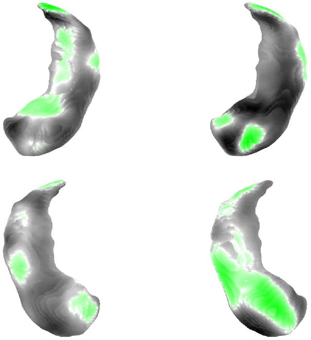
Figure 3 illustrates the determinant of the Jacobian of the translated left to right alignment averaged over the population on the between-group template. The left and right panels respectively provide the bottom and top views of the between-group template. The green/yellow color denotes regions where the right hippocampus is expanded relative to the left hippocampus. The grey/black color denotes regions where the right hippocampus is shrunk relative to the left hippocampus. To perform statistical analysis, we collect the differences between the determinants of the Jacobian within each subfield of the between-group template (Fig. 4) for the left to right and right to left alignments, and use a signed-rank test to accept of reject symmetry. The p-values are respectively <0.0001, <0.0001, and 0.0147 within the sub-fields of subiculum, CA1, and the rest. It suggests that the shape of the left and right hippocampi is statistically significantly asymmetric everywhere, particularly in the subfields of subiculum and CA1.

Fig. 3.

Figure shows the Jacobian of the averaged deformation between left and right hippocampi in the bottom and top views of the between-group template, respectively

Fig. 4.

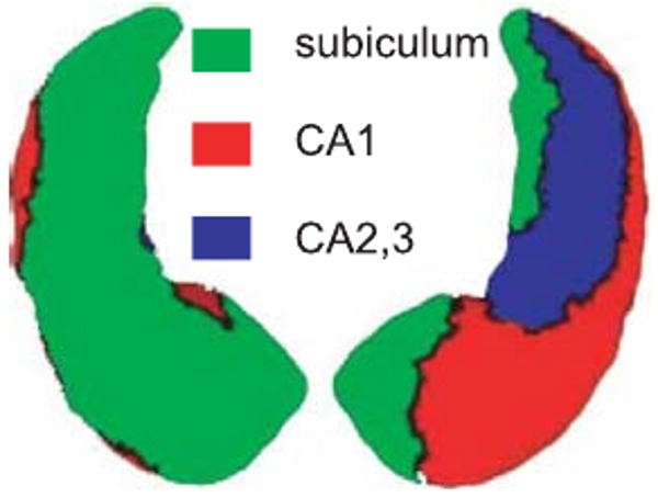
Subfields of the between-group template. Green, red, and blue denote the subfields of subiculum, CA1, CA2 and CA3

6.2 Image Translation

Our second experiment is close to the general scheme described in Fig. 1, and provides a second illustration of the potential uses of the method.

The dataset we have used consists in 3D images of left hippocampi extracted from data collected for a study of depression in children [26]. The subjects are twins, each pair being classified either as control or as HR/MDD (high risk/mental depression disorder). In the HR/MDD pairs, one twin suffers from mental depression, the other one being considered as high risk. For control pairs, no sibling is affected by depression.

The experimental illustration we propose would correspond, in a larger scale study, to a setting designed to test whether the relation between the shapes of the hippocampi has specific features for an HR/MDD pair, compared to controls. The computations we describe are based on 6 pairs of control and 6 pairs of HR/MDD, to which is added a between-group template shape (not part of any of the 12 pairs).

In reference to Fig. 1, each pair forms a group at the lowest level (we therefore have 12 groups). The within-group template is a randomly selected sibling in the control pairs, and the high risk subject in the HR/MDD pairs. Let pair k be ordered as (I_k0, I_k1), for k = 1, …, 12, I_k0 being the within-group template.

The first step of the analysis consists in computing the geodesic between I_k0 and I_k1 for each k. The algorithm used for this step is the one described in [37], which has the property of directly optimizing with respect to the initial momentum, which is the quantity of interest here. At the end of this first step, we have obtained a sequence of scalar fields, z₁, …, z₁₂, such that the initial momentum of the deformation from I_k0 to I_k1 is given by m_k = z_kN_k0, N_k0 being the oriented unit normal to the level sets of I_k0 (cf. (13)).

Step 2 of the procedure (which is independent from Step 1) consists in computing the geodesics between the within-group templates, I_k0, and the between-group template, I_temp. This provides new scalar fields, ζ₁, …, ζ₁₂, such that μ_k = ζ_kN_k0 is the initial momentum of the geodesic between I_k0 and I_temp.

We can now run Step 3, which parallel translate the momenta m_k from I_k0 to I_temp along the geodesics estimated at Step 2. This requires using, for each k, the procedure described in Algorithm 3 with I = I_k0, ξ = −〈∇I_k0, Kμ_k〉 and η = −〈∇I_k0, Km_k〉. This results in new momenta m̃₁, m̃₁₂, each of them aligned with the end point of the geodesic estimated by matching I_k0 to I_temp.

There is a small issue here. Since we use an inexact matching procedure, this end point (denote it Ĩ_k0) does not exactly coincides with I_temp. This had a minor effect in our experiments, because Ĩ_k0 turns out to be very close to the between-group template. However, to ensure that the transported momentum is exactly aligned with the template, we have used the simple correction procedure (Algorithm 4), with m = m̃_k0, I = Ĩ_k0, J = I_temp.

Algorithm 4 Small alignment of the momentum from an image to another

0. Input are two images I and J (J and I are assumed to be similar) and a momentum m aligned with I.

1. Compute v = Km, and the infinitesimal variation of v on J : ξ = − 〈J, v〉.

2. Let the aligned momentum be m0 = z0NJ where NJ is the oriented unit normal to the level sets of J and z0 is provided by the lifting procedure, Sect. 4.3.

The final step of the procedure consisted in averaging on the first hand the momenta that corresponded to the relation within controls pairs, and on the second hand the momenta for the HD/MDD pairs. This resulted in two averaged momenta (say z̄₀ and z̄₁) which are both aligned with the between-group template. They are visualized in Fig. 7. From these two momenta, we can compute two deformations, ϕ̄₀ and ϕ̄₁ by solving the EPDiff equation. Applying these deformations to the between-group template creates two shapes, which can be considered as average deformations for control and HR/MDD pairs respectively. They are visualized in Fig. 5, superimposed with the template. Finally, Fig. 6 provides a visualization of the determinant of the Jacobian of ϕ̄₀ and ϕ̄₁.

Fig. 7.

Momenta of the two averaged within-pair deformations, with the control group on the left and the HR/MDD group on the right. White correspond to a zero value, green to a positive value and dark to a negative value

Fig. 5.

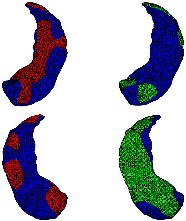
Two different views of the superposition of the between-group template (in blue) and its average variation for the control group (left, in red) and for the HR/MDD group (right, in green)

Fig. 6.

Logarithm of the Jacobian of the two averaged within-pair deformations, with the control group on the left and the HR/MDD group on the right. White correspond to a zero value, green to a positive value and dark to a negative value

Our third example is an experiment using ultrasonic cardiac images. The images are 3D, although with a very low resolution on the third dimension (6 sections). The experiments are based on the following three images, associated to two subjects: I₀ provides an image of Subject 1's heart in end-diastolic position. It is considered here as a within-group template; I₁ is an image of Subject 1's heart in end-systolic position. The between-group template image, I_temp, is the image of Subject 2's heart in end-diastolic position.

We have first registered I₁ to I₀ yielding an initial momentum represented by z₁ (from I₀ to I₁). We have then computed the geodesic between I₀ and I_temp and translated z₁ along it. Let $z_1^{\prime }$ be the result of this operation: this a new momentum, aligned with I_temp, which therefore characterizes a variation of this template. By definition, this variation can be visualized by solving the EPDiff evolution equation starting from the template with initial momentum $z_1^{\prime }$. This provides a new, synthetic, image, $I_1^{\prime }$ which should, if the operation has been successful, have the same relation to the template as I₁ had with I₀. In our case, it should look like a heart in end-systolic position. The results of this computation are provided in Fig. 8. In Fig. 9, the result of coadjoint transport for the same triplet is provided. Coadjoint transport can be seen to provide larger deformations than parallel transport. This is a fact that has been confirmed in most of our experiments.

Fig. 8.

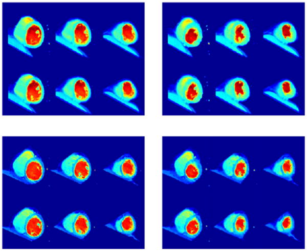
Extrapolation by parallel translation of the systolic shape of Heart 2 (lower-right) given diastolic (upper-left) and systolic (upper-right) shapes of Heart 1 and diastolic shape of Heart 2 (lower-left). Each image provides 6 sections of cardiac ultrasound images

Fig. 9.

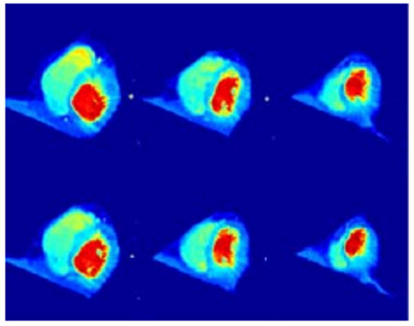
Extrapolation by coadjoint transport for the same dataset as Fig. 8

7 Conclusion

In this paper, we have presented new methods in order to translate the deformation signatures provided by Diffeomorphic Pattern Matching from a given reference frame (template) to another one. We have discuss two options: coad-joint transport and parallel translation. The latter approach requires solving an evolution equation along a geodesic leading from the first template to the second one, for which we suggest using a discretization using Jacobi fields.

Our early experimental results demonstrate that the approach indeed succeeds in transporting shape variations and the signatures that characterize them. Further developments will include large scale longitudinal studies of brain images and times series of heart motion.

Biographies

Laurent Younes is the former student of the Ecole Normale Supérieure in Paris, Laurent Younes was awarded the Ph.D. from the University Paris Sud in 1989, and the thesis advisor certification from the same university in 1995. He was a junior, then senior researcher at CNRS (French National Research Center) from 1991 to 2003. He is now professor in the Department of Applied Mathematics and Statistics at Johns Hopkins University. Here is a core faculty member of the Center for Imaging Science and of the Institute for Computational Medicine at JHU. His main research interests are on statistical analyses of images and shapes, and on mathematical models for shape deformations and shape spaces.

Anqi Qiu received her Ph.D. degree in Electrical and Computer Engineering from Johns Hopkins University in 2006. She also holds M.S. degrees in Biomedical Engineering and Applied Mathematics and Statistics. From 2007, she joined National University of Singapore as assistant professor. Her research interests focus on medical imaging analysis.

Rpaimond L. Winslow is Professor of Biomedical Engineering at Johns Hopkins University School of Medicine. He also directs the Institute for Computational Medicine at Johns Hopkins University. His interests are in integrative modeling of heart function in health and disease. This includes mathematical and computational modeling of signal transduction, metabolism, ion channels, intracellular calcium cycling, and force generation within the cardiac myocyte. His lab has also measured and modeled the structure of the cardiac ventricles using diffusion tensor MR imaging and finite-element modeling methods.

Michael I. Miller is the Herschel and Ruth Seder Professor of Biomedical Engineering, Professor of Electrical and Computer Engineering and Director of Center for Imaging Science at Johns Hopkins University, Baltimore, MD. Throughout his career his research interests have focused on image understanding and computer vision; medical imaging and computational anatomy.

Previous to his current position, Michael Miller was the Newton R. and Sarah Louisa Glasgow Professor in Biomedical Engineering at the Washington University Department of Electrical Engineering. From 1995–2000 he was the director of the Army Center for Imaging Science, an Academic Center of Excellence consisting of 7 universities dedicated to the development of new methods for image understanding and automated target recognition. He has been a visiting professor at several over several years at the Ecole Normale in France and a visiting professor at Brown University.

Michael Miller is a Fellow of the American Institute for Medical and Biological Engineering. He is a Presidential Young Investigator Award Winner and is the recipient of International Order of Merit; International Man of the Year, Warrant of Proclamation and Medal of Recognition from the International Biographical Centre, Cambridge England; and Universal Award of Accomplishment. He has been an invited and plenary speaker at numerous national and international meetings. In 2002 he was recognized by in-cites as having the greatest increase in citation rates in the field of Engineering for his work in Computational Anatomy.

Michael Miller received a B.S.E.E., Electrical Engineering, State University of New York at Stony Brook, an M.S. in Electrical Engineering from Johns Hopkins University and a Ph.D. in Biomedical Engineering also from Johns Hopkins University, Baltimore, MD.

References

- 1.Arnold VI. Sur un principe variationnel pour les ecoulements stationnaires des liquides parfaits et ses applications aux problèmes de stanbilité non linéaires. J Méc. 1966;5:29–43. [Google Scholar]
- 2.Arnold VI. Mathematical Methods of Classical Mechanics. 2nd edn. 1989 Springer; Berlin: 1978. [Google Scholar]
- 3.Ashburner J, Friston KJ. Voxel based morphometry—the methods. Neuroimage. 2000;11(6):805–821. doi: 10.1006/nimg.2000.0582. [DOI] [PubMed] [Google Scholar]
- 4.Avants B, Gee J. Shape averaging with diffeomorphic flows for atlas creation. Proceedings of ISBI 2004. 2004 [Google Scholar]
- 5.Bajcsy R, Broit C. Matching of deformed images. The 6th International Conference in Pattern Recognition; 1982. pp. 351–353. [Google Scholar]
- 6.Beg MF, Miller MI, Trouvé A, Younes L. Computing large deformation metric mappings via geodesic flows of diffeomorphisms. Int J Comput Vis. 2005;61(2):139–157. [Google Scholar]
- 7.Boothby W. An Introduction to Differentiable Manifolds and Riemannian Geometry. Original edition 1986 Academic Press; San Diego: 2002. [Google Scholar]
- 8.Camassa R, Holm DD. An integrable shallow water equation with peaked solitons. Phys Rev Lett. 1993;71:1661–1664. doi: 10.1103/PhysRevLett.71.1661. [DOI] [PubMed] [Google Scholar]
- 9.Christensen GE, Rabbitt RD, Miller MI. Deformable templates using large deformation kinematics. IEEE Trans Image Process. 1996 doi: 10.1109/83.536892. [DOI] [PubMed] [Google Scholar]
- 10.Cotter CJ, Holm DD. Discrete momentum maps for lattice epdiff. Technical Report. 2006 ArXiv:math.NA/0602296. [Google Scholar]
- 11.Dupuis P, Grenander U, Miller M. Variational problems on flows of diffeomorphisms for image matching. Q Appl Math. 1998;56:587–600. [Google Scholar]
- 12.Gee JC, Fabella BA, Fernandes BI, Turetsky BI, Gur RC, Gur RE. New experimental results in atlas-based brain morphometry. SPIE Medical Imaging. 1999 [Google Scholar]
- 13.Golland P, Grimson EW, Shenton ME, Kikinis R. Lecture Notes in Computer Sciences. Vol. 2082. Springer; Berlin: 2001. Deformation analysis for shape based classification. In: Information Processing in Digital Imaging (IPMI 2001) [Google Scholar]
- 14.Grenander U, Miller MI. Computational anatomy: An emerging discipline. Q Appl Math. 1998;LVI(4):617–694. [Google Scholar]
- 15.Helm PA, Younes L, Beg MF, Ennis DB, Leclercq C, Faris OP, McVeigh E, Kass D, Miller MI, Winslow RL. Evidence of structural remodeling in the dyssynchronous failing heart. Circ Res. 2005;98:125–132. doi: 10.1161/01.RES.0000199396.30688.eb. [DOI] [PubMed] [Google Scholar]
- 16.Holm DD, Marsden JE, Ratiu TS. The Euler–Poincaré equations and semidirect products with applications to continuum theories. Adv Math. 1998;137:1–81. [Google Scholar]
- 17.Holm DR, Ratnanather JT, Trouvé A, Younes L. Soliton dynamics in computational anatomy. Neuroimage. 2004;23:S170–S178. doi: 10.1016/j.neuroimage.2004.07.017. [DOI] [PubMed] [Google Scholar]
- 18.Joshi S, Miller M. Landmark matching via large deformation diffeomorphisms. IEEE Trans Image Process. 2000;9(8):1357–1370. doi: 10.1109/83.855431. [DOI] [PubMed] [Google Scholar]
- 19.Ma J, Miller MI, Trouvé A, Younes L. Technical Report, Center for Imaging Science. Johns Hopkins University; 2007. Bayesian template estimation in computational anatomy. [Google Scholar]
- 20.Marsden JE, Ratiu TS. Introduction to Mechanics and Symmetry. Springer; Berlin: 1999. [Google Scholar]
- 21.Miller MI, Priebe C, Qiu A, Fischl B, Kolasny A, Brown T, Park Y, Busa E, Jovicich J, Yu P, Dickerson B, Buckner RL. the Morphometry BIRN: Collaborative computational anatomy: The perfect storm for mri morphometry study of the human brain via diffeomorphic metric mapping. Proc Natl Acad Sci. 2007 doi: 10.1002/hbm.20655. [DOI] [PMC free article] [PubMed] [Google Scholar]
- 22.Miller MI, Trouvé A, Younes L. On the metrics Euler-Lagrange equations of computational anatomy. Annu Rev Biomed Eng. 2002;4:375–405. doi: 10.1146/annurev.bioeng.4.092101.125733. [DOI] [PubMed] [Google Scholar]
- 23.Miller MI, Trouvé A, Younes L. Geodesic shooting for computational anatomy. J Math Imag Vis. 2006;24(2):209–228. doi: 10.1007/s10851-005-3624-0. [DOI] [PMC free article] [PubMed] [Google Scholar]
- 24.Miller MI, Younes L. Group action, diffeomorphism and matching: a general framework. Int J Comput Vis. 2001;41:61–84. Originally published in electronic form in: Proceeding of SCTV 99, http://www.cis.ohio-state.edu/∼szhu/SCTV99.html. [Google Scholar]
- 25.Pennec X, Ayache N. Uniform distribution, distance and expectation problems for geometric features processing. J Math Imaging Vis. 1998;9(1):49–67. [Google Scholar]
- 26.Priebe C, Park Y, Miller MI, Botteron K, Mohan N. Statistical analysis of twin populations using dissimilarity measurements in hippocampus shape space. J Biomed Biotechnol. 2008 doi: 10.1155/2008/694297. to appear. [DOI] [PMC free article] [PubMed] [Google Scholar]
- 27.Thirion JP. Image matching as a diffusion process: an analogy with maxwell's demons. Med Image Anal. 1998;2(3):243–260. doi: 10.1016/s1361-8415(98)80022-4. [DOI] [PubMed] [Google Scholar]
- 28.Thirion JP. Diffusing models and applications. In: Toga AW, editor. Brain Warping. Academic Press; San Diego: 1999. pp. 144–155. [Google Scholar]
- 29.Thirion JP, Calmon G. Deformation analysis to detect and quantify active lesions in 3D medical image sequences. IEEE Trans Image Anal. 1999;18(5):429–442. doi: 10.1109/42.774170. [DOI] [PubMed] [Google Scholar]
- 30.Thompson PM, Mega MS, Vidal S, Rapoport JL, Toga AW. Information Processing in Digital Imaging (IPMI 2001), Lecture Notes in Computer Sciences. Vol. 2082. Springer; Berlin: 2001. Detecting disease-specific patterns of brain structure using cortical pattern matching and a population-based probabilistic brain atlas. [DOI] [PMC free article] [PubMed] [Google Scholar]
- 31.Thompson PM, Toga AW. Detection, visualization and animation of abnormal anatomic structure with a deformable probabilistic brain atlas based on random vector field transformations. Med Image Anal. 1996/7;1(4):271–294. doi: 10.1016/s1361-8415(97)85002-5. [DOI] [PubMed] [Google Scholar]
- 32.Trouvé A. Infinite dimensional group action and pattern recognition. Technical Report, DMI, Ecole Normale Supérieure. 1995 [Google Scholar]
- 33.Trouvé A. Diffeomorphism groups and pattern matching in image analysis. Int J Comput Vis. 1998;28(3):213–221. [Google Scholar]
- 34.Trouvé A, Younes L. Local geometry of deformable templates. SIAM J Math Anal. 2005;37(1):17–59. [Google Scholar]
- 35.Vaillant M, Glaunès J. Proceedings of Information Processing in Medical Imaging (IPMI 2005). Lecture Notes in Computer Science. Vol. 3565. Springer; Berlin: 2005. Surface matching via currents. [DOI] [PubMed] [Google Scholar]
- 36.Vaillant M, Miller MI, Trouvé A, Younes L. Statistics on diffeomorphisms via tangent space representations. Neuroimage. 2004;23(S1):S161–S169. doi: 10.1016/j.neuroimage.2004.07.023. [DOI] [PubMed] [Google Scholar]
- 37.Younes L. Jacobi fields in groups of diffeomorphisms and applications. Q Appl Math. 2007;65:113–134. [Google Scholar]